Article

Assessment on Hydrologic Response by Climate Change in the Chao Phraya River Basin, Thailand

1
School of Urban and Environmental Engineering, Ulsan National Institute of Science and Technology, Ulsan 689-798, Korea
2
Water Institute, 1689beon-gil 125, Yuseong-Daero, Yuseong-gu, Daejeon 305-730, Korea
3
Department of Environmental Engineering, Dong-A University, Busan 604-714, Korea
4
Environmental and Plant Engineering Research Institute, Korea Institute of Civil Engineering and Building Technology (KICT), 283, Goyangdae-Ro Ilsanseo-Gu, Goyang-Si, Gyeonggi-Do 10223, Korea
5
Department of Environmental Science and Engineering, Gwangju Institute of Science and Technology, Gwangju 500-712, Korea
*
Authors to whom correspondence should be addressed.
These authors contributed equally to this work.
Water 2015, 7(12), 6892-6909; https://doi.org/10.3390/w7126665
Submission received: 12 October 2015 / Revised: 25 November 2015 / Accepted: 26 November 2015 / Published: 4 December 2015
(This article belongs to the Special Issue Water Resource Variability and Climate Change)

Abstract

:
The Chao Phraya River in Thailand has been greatly affected by climate change and the occurrence of extreme flood events, hindering its economic development. This study assessed the hydrological responses of the Chao Phraya River basin under several climate sensitivity and greenhouse gas emission scenarios. The Soil and Water Assessment Tool (SWAT) model was applied to simulate the streamflow using meteorological and observed data over a nine-year period from 2003 to 2011. The SWAT model produced an acceptable performance for calibration and validation, yielding Nash-Sutcliffe efficiency (NSE) values greater than 0.5. Precipitation scenarios yielded streamflow variations that corresponded to the change of rainfall intensity and amount of rainfall, while scenarios with increased air temperatures predicted future water shortages. High CO2 concentration scenarios incorporated plant responses that led to a dramatic increase in streamflow. The greenhouse gas emission scenarios increased the streamflow variations to 6.8%, 41.9%, and 38.4% from the reference period (2003–2011). This study also provided a framework upon which the peak flow can be managed to control the nonpoint sources during wet season. We hope that the future climate scenarios presented in this study could provide predictive information for the river basin.

1. Introduction

Current environmental changes due to either natural or anthropogenic influences are creating a significant impact on natural resources and the living conditions of humans [1]. In particular, as a critical natural resource, water bodies have been subjected to pollution and are reaching scarcity levels around the globe [2,3]. Climate change is a key factor that has greatly affected water resources, due to its uncertainty and variability [4,5,6]; the intensities and frequencies of rainfall have been fluctuating over the years, thereby changing the spatiotemporal distributions of water resources [7]. Furthermore, it is apparent that climate change influences a change in water quality by modifying the surface and groundwater components [8,9]. Floods and droughts brought about by climate change may also lead to a change in water quality by increasing the effects of erosion or dilution [8,10,11].
There are several signs that the varying rainfall intensity has caused a change in climate change factors. These change factors include the increasing global surface temperature and significant local impacts such as high-magnitude floods, prolonged droughts, flow variability, temperature rise, and decreased rainfall [12,13,14]. As such, there is a need to change the perception of climate change and its uncertainty and vulnerability since its weaknesses should be prioritized. Though a certain level of uncertainty has always existed in water resource management and planning, alternative approaches to manage water resources have been proposed, such as creating climate change scenarios with respect to speed and intensity of changes in baseline conditions [15,16]. In addition, though it is difficult to mitigate the effect of climate on water quantity since policy makers should obtain scientific and predictive information, for effective water resources management, the accurate prediction of water quantity and quality is a necessary response to the climate change scenario [17,18,19].
The Chao Phraya River, a major river basin in the Mekong subregion and the largest watershed in Thailand, serves mostly as a source for irrigation water and a transportation route in Central Thailand [20]. Over the years, climate change has greatly affected the river, which may subsequently hinder the economic development and the eradication of poverty in adjacent countries [21]. The Chao Phraya River basin has experienced extreme floods, which has brought about the subsequent contamination water used for human consumption [22], health problems [23,24], and economic loss on Thai Rice exports [25]. For example, the flood event that occurred in 2011 caused 813 fatalities nationwide and $45.7 billion in economic damages and losses [26,27]. This event prompted several researchers to conduct further case studies in different fields, including disaster management [28] and medicine [29,30].
Water management of irrigation water is very important for the Chao Phraya River basin because it is one of the world’s major agricultural producers, having a cultivated area of approximately 51% (cropland) [31,32,33]. However, climate change has also played a significant role in the rate of landuse changes in the basin [34]. Farmers respond to weather conditions by changing crops seasonally, the timing of planting and harvesting, and other daily activities [35]. In cases such as this, there remains a need to understand the characteristics of the basin and its hydrological response to climate change.
To address the issues presented by extreme flood events and climate change, this study investigates the impact of climate change scenarios on the basin. The aims of this investigation are thus to: (1) calibrate and validate the water quantity in the Chao Phraya River basin using the Soil and Water Assessment Tool (SWAT) model; and (2) assess hydrological responses under hypothetical climate sensitivity scenarios and greenhouse gas emission scenarios. The results of this research will both help improve the foundation of water resource management based on these climate change scenarios and also provide an evaluation of highly variable climate changes on the basin.

2. Methodology

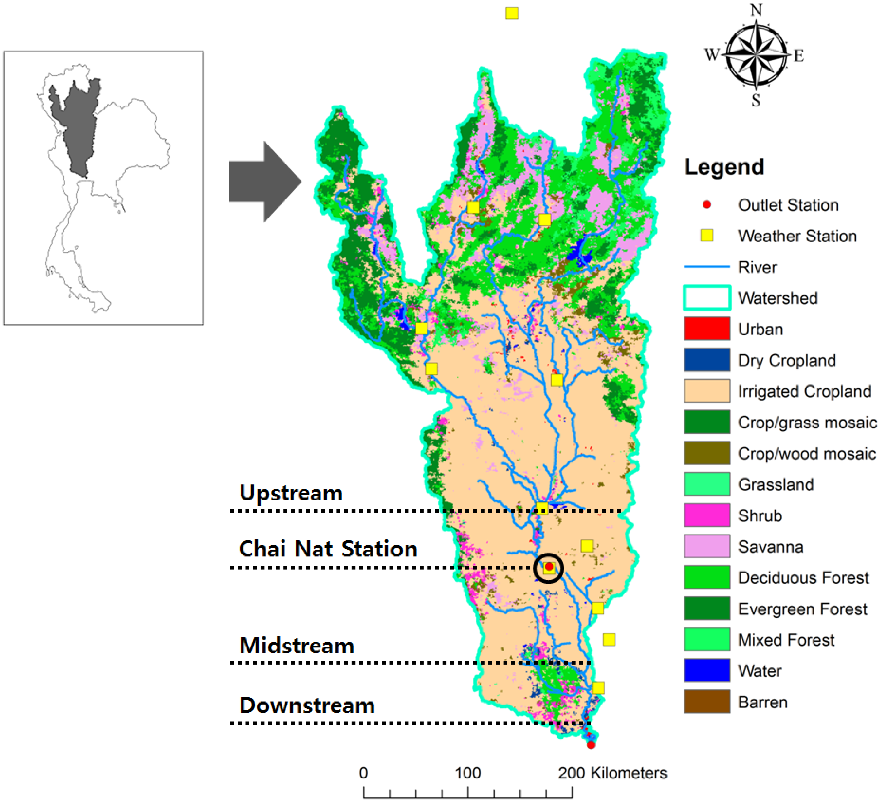
2.1. Site Description

The Chao Phraya River is an important water resource that supplies water to irrigated, urban, and domestic areas of the central part of Thailand [36]. Figure 1 presents the land use classes used in the SWAT model. It also includes the weather and outlet stations of the Chao Phraya River basin. The basin has 51.66% agriculture area, which depends on the main river and its tributaries to cultivate crops, such as rice, sugarcane, and corn. The river has four main tributaries: the Wang, Yom, Ping, and Nan Rivers and a significant lateral tributary, the Pasak River. The river drains an area of approximately 160,000 km2 (98° E–103° E, 13° N–20° N), covering 30% of the country, and receives annual precipitation of about 1,179 mm/year and an average discharge of 196 m3/s at Chai Nat Station [37]. The basin is in a tropical climate, and is influenced by northeast and southwest monsoons. The northeast monsoon brings in cool and dry air from November to February, whereas the southwest monsoon brings very humid air, thus causing heavy rains from May to October [38].
Figure 1. Chao Phraya River basin is shown in the map. It includes the locations of the twelve weather stations (yellow squares) of the basin as well as the outlet stations (red circles) of the river, which also served as monitoring stations. Chai Nat Station has been chosen for the SWAT model simulation of the streamflow.
Water 07 06665 g001

2.2. SWAT Model

The Soil and Water Assessment Tool (SWAT) is watershed model that can be applied to simple and complex watersheds. It is a continuous-time model that operates on a daily time step and was developed for the USDA Agricultural Research Service (ARS) to predict the impact of management on water, sediment, and agricultural chemical yields in large complex watersheds [39]. The model is physically-based, uses readily available inputs, is computationally efficient, and is able to continuously simulate long-term impacts. Major model components include hydrology, weather, soil, temperature, plant growth, nutrients, pesticides, and land management. The SWAT model divides the watershed into multiple subwatersheds, which are then further subdivided into hydrologic response units (HRUs) that consist of homogenous land use, management, and soil characteristics. Models calibrated using watershed and water quality data have been used to forecast water quantity/quality in response to climate change scenarios; the SWAT model has been widely used to predict water quantity and quality in response to various management and climate scenarios [40,41,42,43,44,45,46,47,48,49,50,51].

2.3. Model Application

To construct the Chao Phraya River basin model, a model database was compiled using topographical data, consisting of a digital elevation map, landuse, soil and river basin, meteorological data (e.g., precipitation, and maximum and minimum temperature), and observed monitoring data (e.g., flow discharge). The topographical data included a digital elevation model (DEM) in GeoTiff grid tiles (5° × 5° tiles) created from a water database [52]; the data was derived from USGS/NASA Shuttle Radar Topography Mission (SRTM) data with a 90 m resolution. The land use data has a spatial resolution of 1 km that included 14 classes of landuse representations from the USGS Global Land Cover Characterization (GLCC) database [53]. There were also 14 soil types in the soil grid provided by the Food and Agriculture Organization of the United Nations [54]. We also obtained nine-year meteorological data (2003–2011) from the Thai Meteorological Department, which included daily precipitation and maximum/minimum temperatures from 12 stations within the Chao Phraya River basin.
The SWAT model was able to delineate an area of 119,663 km2 of the Chao Phraya River basin. Figure 1 illustrates the Chao Phraya River basin built by SWAT. Landuse classes of the basin are listed in Table 1, showing that the basin is mainly comprised of agriculture area and broadleaf forest. The table also indicates that half of the area used for agriculture was irrigated cropland and pasture (CRIR). Streamflow was monitored at the Chai Nat Station located in Chai Nat province. The observed flow data of the said station was stable and were acquired from the Royal Irrigation Department Computer Center in Sanphaya, Chai Nat.
Table 1. Area and percentage of land cover in the Chao Phraya River basin.
LanduseDefinitionArea (ha)Percentage (%)
CRIRIrrigated cropland and pasture6,181,83151.66
FODBDeciduous broadleaf forest1,947,50916.27
FOEBEvergreen broadleaf forest1,503,65312.57
SAVASavanna1,038,5678.68
FOMIMixed forest495,3014.14
CRWOCropland/woodland mosaic294,7062.46
SHRBShrubland270,0812.26
WATBWater bodies113,7310.95
CRDYDryland cropland and pasture79,3650.66
URMDUrban residential medium density37,8200.32
GRASGrassland30600.03
CRGRCropland/grassland mosaic3810
BSVGBarren or sparsely vegetated2490
Watershed11,966,254100

2.4. Sensitivity Analysis

The Latin Hypercube—One-factor-At-a-Time (LH-OAT) method is a sensitivity analysis technique that combined the robustness of the Latin Hypercube (LH) sampling method and a one-factor-at-a-time (OAT) design [55]. It searches for good performance using a limited parameter number of important factors for model calibration and model output for a particular basin. LH is a stratified sampling method developed by McKay et al. [56] and is based on the Monte Carlo simulation; the OAT design was developed by Morris [57] and is used to observe the changes in the output by changing a particular input. LH-OAT method firstly divides the range of the parameters into segments then takes LH samples from each parameter to create parameter sets. The OAT design can then achieve global sensitivity by changing an entire parameter range using the LH samples [58]. Table 2 shows the 15 SWAT model parameters that were subjected to sensitivity analysis.
Table 2. Soil and water assessment tool (SWAT) model parameters used for the sensitivity analysis.
NameDefinitionRangeProcess
Cn2Soil Conversion Service (SCS) runoff curve number for moisture condition 235–98Runoff
Alpha_BfBaseflow alpha factor (days)0.00–1.00Groundwater
Rchrg_DpDeep aquifer percolation fraction0.00–1.00Groundwater
EscoSoil evaporation compensation factor 0.00–1.00Evaporation
RevapmnThreshold depth of water in the shallow aquifer for percolation to the deep aquifer (mmH2O)0–500Groundwater
Ch_K2Effective hydraulic conductivity in main channel alluvium (mm/h)−0.01–150Channel
GwqmnThreshold depth of water in the shallow aquifer required for return flow to occur (mm)0–5000Soil
Sol_AwcAvailable water capacity of the soil layer (mm/mm soil)0–100Soil
Sol_ZMaximum canopy index Soil depth0–3000Soil
Gw_RevapGroundwater “revap” coefficient0.02–0.2Groundwater
SurlagSurface runoff lag coefficient0.00–10.00Runoff
BlaiLeaf area index for crop0.00–1.00Crop
SlopeAverage slope steepness (m/m)0.0001–0.6Geomorphology
CanmxMaximum canopy index0.00–10.00Runoff
EpcoThreshold depth of water in the shallow aquifer to percolation to the deep aquifer (mmH2O)0.00–1.00Evaporation

2.5. Performance Assessment

We applied a coefficient of determination (R2), Nash-Sutcliffe efficiency (NSE), and root mean square error (RMSE) to evaluate the model performance. R2 evaluated how accurate the simulated values were compared to the observed values and is defined as the squared value of Bravais-Pearson’s coefficient of correlation (r) [59,60]. It depicts the strength between the simulated and observed data and the direction of the linear relation. R2 is expressed as the squared ratio between the covariance and the multiplied standard deviation of the observation and simulated values [61]. NSE measures the goodness of fit and describes the variance between the simulated and observed values [62]. NSE values can differ from negative values up to less than one [63]. Generally, the calibration and validation values of the SWAT model are considered to be acceptable or satisfactory performances when NSE is within the range of 0.5 and 0.65, 0.65–0.75 is considered satisfactory, while 0.75–1.00 indicate a very good performance [64,65,66]. Table 3 presents the performance ratings for NSE, as suggested by Moriasi et al. (2007). Lastly, RMSE was used to assess the validity of the model in this study. It measures the square root of the distance between the observed and predicted values and gives an estimate of the variability of the model compared to the observations [49]. The desired value for RMSE is 0, which depicts a perfect simulation, with lower values representing better performance [67].
Table 3. General performance rating for the recommended statistics for monthly time step [68].
Performance RatingNSE
Very good0.75 < NSE ≤ 1.00
Good0.65 < NSE ≤ 0.75
Satisfactory0.50 < NSE ≤ 0.65
UnsatisfactoryNSE ≤ 0.50

2.6. Climate Change Scenarios

We applied a Special Report on Emission Scenario (SRES) to assess the hydrological response using a future climate change scenario. We applied the Commonwealth Scientific and Industrial Research Organisation (CSIRO) Mark 3.5 (Mk3.5) (CSIRO Atmospheric Research, Melbourne, Victoria, Australia)from the CSIRO Marine and Atmospheric Research in Australia as the future climate change model since it provides daily meteorological data for a long period for each climate change scenario. The future climate scenarios from the Intergovernmental Panel on Climate Change (IPCC) (A2, A1B, and B1) were chosen as its outputs (greenhouse gas emission scenarios) [69,70]. Mk3.5 is based on CSIRO Mark 3.0 (Mk3.0), a prior model version that has a fully coupled ocean-atmosphere system [71]. It is a spectral model that was developed to use the horizontal spectral resolution T63 [1.875° EW × 1.875° NS] with 18 vertical levels, and to remove the cold bias of Mk3.0 due to the rising of global air temperature [72].
Four different qualitative storylines were developed by IPCC that represented the different demographic, social, economic, technological, and environmental developments of the communities [73,74]. SRES scenarios A1B, A2, and B1 were chosen for this study [75,76]. A1B is under the A1 storyline and scenario family, which emphasizes globalization. A1B is described as a balance across all energy sources that do not rely heavily on a specific source [40]. The A2 scenario describes a very heterogeneous world with slower economic growth and technological advancement compared to the other storylines. Lastly, the B1 scenario stresses on rapid economic change towards service and information, social and environmental sustainability, improved equity, and global solutions without additional climate initiatives [77].
The potential future climate included a set of gridded map layers for the daily precipitation and air temperature for 2051–2059, based on the output from a set of SRES. GCM produced the climate data applied in this study; however, the coarse resolution of GCM will reduce the accuracy of the results. An interpolation method was implemented to convert the GCMs of the 12 meteorological stations to finer regional resolutions. The converted climate data was then downscaled and used as weather inputs for the SWAT model.
The change factor method, a downscaling technique, was used to adjust the observed daily temperature and daily precipitation using Equations (1) and (2), respectively. The daily temperature at the 2059 horizon was obtained by adding the difference of mean daily temperature in 2059 horizon predicted by the climate model and mean temperature of the reference period (2003–2011) to the observed daily temperature, obtained using Equation (1) [78]. The daily precipitation was calculated by multiplying the observed daily precipitation with the ratio of the mean projected daily precipitation at the 2059 horizon, and the mean precipitation of the reference period, as described in Equation (2) [79].
T a d j , 2059 , d = T o b s , d +   (   T   ¯ C M , 2059 , m     T   ¯ C M , r e f , m )
P a d j , 2059 , d = P o b s , d ×   (   P   ¯ C M , 2059 , m   ÷   P   ¯ C M , r e f , m )
where Tobs,d and Pobs,d are the observed daily temperature and precipitation, TCM,2059,m and PCM,2059,m are the projected daily temperature and precipitation at the 2059 horizon obtained by the climate model, TCM,ref,m and PCM,ref,m are the temperature and precipitation during the reference period (2003–2011), and Tadj,2059,d and Padj,2059,d are the daily temperature and precipitation at the 2059 horizon. The averages of the temperature and precipitation from the 12 meteorological stations were the data used for the TCM,ref,m and PCM,ref,m, respectively. The strength of the change factor (CF) method is similar to the results of factors derived from GCM or Regional Climate Model (RCM).
Table 4 shows the conditions of the hypothetical climate sensitivity scenarios. There were zero changes in precipitation and temperature at the reference point, with CO2 concentrations at 330 ppm. Scenarios 1 to 3 have twice the CO2 concentration (660 ppm) and high variation in the precipitation and air temperature. Scenarios 4 to 7 show variations in the precipitation, while maintaining constant CO2 concentrations and air temperatures. Scenarios 8 to 10 have variations air temperature, while CO2 concentrations and precipitations remain constant. The change factors of the SRES scenarios, A1B, A2, and B1, were also included in the table.
Table 4. Conditions of climate sensitivity scenarios and intergovernmental panel on climate change (IPCC) special report on emissions scenarios relative to the baseline. Scenarios 1–3 are referred to as the CO2 scenarios, 4–7 as precipitation change scenarios, and 8–10 as temperature increase scenarios.
ScenarioCO2 Concentration (ppm)Precipitation Change (%)Temperature (°C)
Baseline33000
1CO2 × 2 = 66000
2CO2 × 2 = 660+200
3CO2 × 2 = 6600+6
4330+100
5330+200
6330−100
7330−200
83300+1
93300+3
103300+6
A1B330+1.0644Max+2.0621
Min+2.4954
A2330+1.0338Max+1.8729
Min+2.2905
B1330+1.0054Max+0.7926
Min+0.6106

3. Results and Discussion

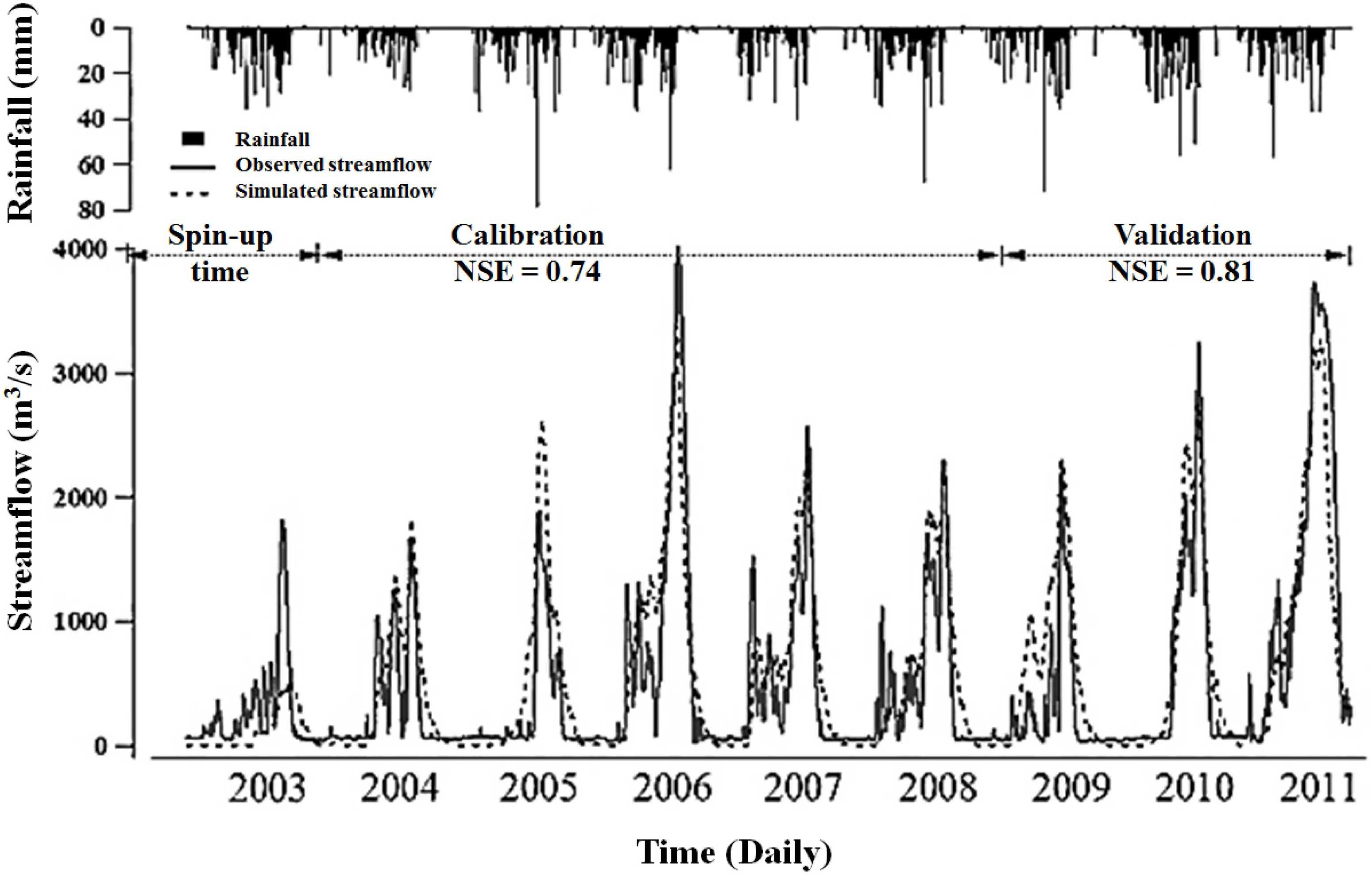
3.1. Model Evaluation

Thirty-five hydrological model parameters of the SWAT model underwent sensitivity and uncertainty analyses (e.g., Parameter solution (Para Sol) and Sequential Uncertainty Fitting (SUFI-2) in SWAT-CUP) to determine the optimal model parameters [80]. The top 11 parameters having sensitivity indices greater than or equal to 0.05 were then selected, as shown in Table 5 [81]. The result of the sensitivity analysis shows that the initial SCS runoff curve number for moisture condition II (CN2) and baseflow alpha factor-baseflow recession (Alpha_Bf) were the most sensitive parameters. They are followed by the deep aquifer percolation fraction (Rchrg_Dp), soil evaporation compensation factor (Esco), threshold depth of water in the shallow aquifer for percolation to the deep aquifer (Revapmn), effective hydraulic conductivity in main channel alluvium (Ch_K2), available water capacity of the soil layer (Sol_AWC), threshold depth of water in the shallow aquifer required for return flow to occur (Gwqmn), depth from soil surface to bottom of layer (Zol_Z), groundwater “revap”coefficient (Gw_Revap), and surface runoff lag coefficient (Surlag). Most parameters are related to either groundwater or soil process. The sensitive flow discharge parameters were then used to calibrate the model.
One of the limitations of this research was having a large watershed model with only 12 meteorological stations and one gauge station to calibrate the streamflow. The available data allowed nine years for the simulation period of the SWAT model. The comparison of daily observed and simulated streamflow during the nine-year (2003–2011) simulation period included a one-year spin up time (2003), a five-year (2004–2008) calibration period, and a three-year (2009–2011) validation period. Results from the statistical evaluation with the two numeric criteria including NSE, R2, and RMSE, are listed in Table 6. Figure 2 shows how well-matched the daily streamflow simulations with the observations were. The NSE values of the daily streamflow simulations for the calibration and validation were 0.74 and 0.81, respectively. On the other hand, the NSE values of the monthly time step were 0.54 and 0.66 for the five-year calibration and three-year validations, respectively. The model evaluation statistics for the streamflow prediction show that there was a fair agreement between the measured and simulated flows, which were confirmed by the R2 and NSE being greater than 0.5 [62].
Table 5. Top 11 parameters yielded by the sensitivity analysis.
RankNameDefinitionSensitivityProcess
1Cn2SCS runoff curve number for moisture condition 21.49Runoff
2Alpha_BfBaseflow alpha factor (days)1.42Groundwater
3Rchrg_DpDeep aquifer percolation fraction0.66Groundwater
4EscoSoil evaporation compensation factor0.48Evaporation
5RevapmnThreshold depth of water in the shallow aquifer for percolation to the deep aquifer (mm H2O)0.22Groundwater
6Ch_K2Effective hydraulic conductivity in main channel alluvium (mm/h)0.20Channel
7GwqmnThreshold depth of water in the shallow aquifer required for return flow to occur (mm)0.18Soil
8Sol_AwcAvailable water capacity of the soil layer (mm/mm soil)0.14Soil
9Sol_ZMaximum canopy index Soil depth0.078Soil
10Gw_RevapGroundwater “revap” coefficient0.06Groundwater
11SurlagSurface runoff lag coefficient0.05Runoff
Table 6. Prediction accuracy for the monthly streamflow in terms of R2, Nash-Sutcliffe efficiency (NSE) and root mean square error (RMSE).
Statistical IndexCalibrationValidation
R20.810.89
NSE0.540.66
RMSE (m3/s)2.5466 × 1033.0224 × 103
Figure 2. Observed and simulated streamflow and the corresponding daily rainfall during a nine-year period (2003–2011). Figure includes a one-year spin-up period (2003), five-year calibration period (2004–2008), and three-year validation period (2009–2011).
Water 07 06665 g002

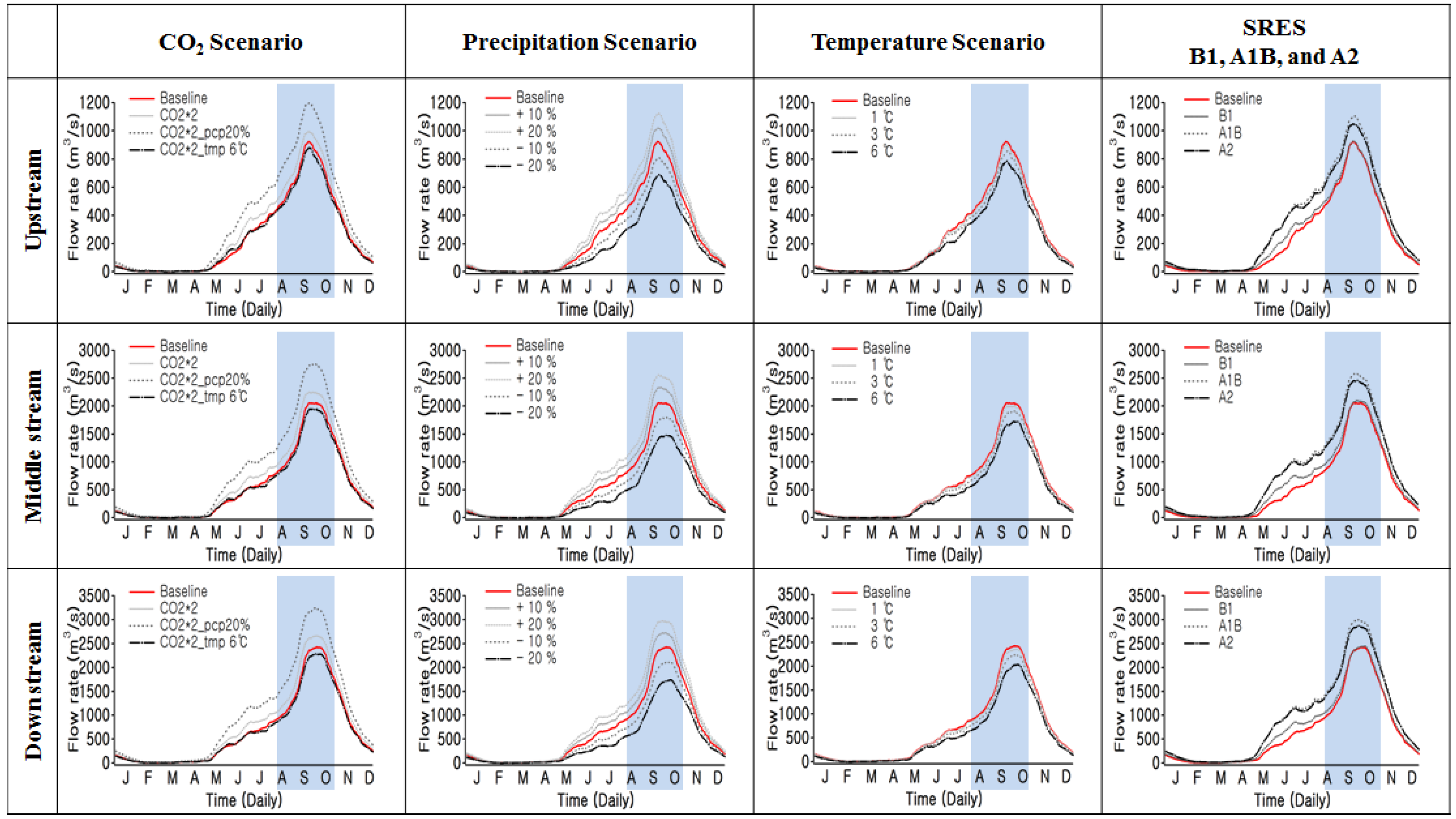
3.2. Climate Sensitivity Scenario

3.2.1. CO2 Concentration

Scenarios 1 to 3 have atmospheric CO2 concentrations of 660 ppm and a change in precipitation and air temperature (Table 7). These three scenarios were related to the stomatal conductance variable, which depends on the atmospheric CO2 concentration [82]. For climate change simulations in the SWAT model, the reduction in stomatal conductance and increase in leaf area index were attributed to an increase in the CO2 concentration [83]. According to the increasing atmospheric CO2 concentration, variation in the streamflow was seen to be affected by the change in evapotranspiration, whereas the hydrological response depends on crop variables [84]. When the stomatal conductance of the vegetation decreases, the evapotranspiration also decreases, thus disturbing the water efficiency of the crops [84,85]. Table 7 shows the predicted relative change (percentage of baseline) in annual average streamflow with respect to the climate change scenario. In the calibration of the Chao Phraya subbasin, the annual average streamflow changed by 16.4% in calibration, another changed by 18.4%, with a maximum of 52.3% and a minimum of 1.6% in the whole basin. Scenario 2 reflects an increase of almost 48% in the annual average streamflow change of the subbasin; another subbasin increased by 52.6%, while the maximum was 128.9% and the minimum was 15.1% in the whole basin. Scenario 3, on the other hand, showed an annual average streamflow change of −5.3% at Chai Nat Station, whereas another site changed by −6.2%, with a maximum of 1.2%, and a minimum of −14.3% in the whole basin.
Table 7. Predicted relative percentage change of annual average streamflow from the baseline under different climate sensitivity scenarios and special report on emission scenario (SRES) (B1, A1B, and A2). It also includes the streamflow change at the Chai Nat Station.
TermsRefClimate Sensitivity ScenarioSRES
Stream-FlowCO2 (%)Precipitation (%)Air Temperature (%)GCM (%)
12345678910B1A1BA2
Chai Nat Station562.816.448−5.315.630−15.8−32.8−3.1−9.3−19.224.741.949.8
Max % change of the basin671.852.3128.91.235.970−7−14.58.28.2−1.3107.8136.5146.4
Min % change of the basin1.31.615.1−14.35.911.6−37.3−71.4−8.2−23.8−53−17.5−1.14.1
Average % change of the basin68.518.452.6−6.216.632.2−16.7−34.5−3.5−10.6−21.419.737.747
Figure 3a–c show streamflow variations of the basin, mostly ranging from −2% to 20%. The spatial variation for CO2 concentration scenario displayed an increasing streamflow change in the southern area of Chao Phraya River basin that is within the range of 20% to 42% (Figure 3a). Scenario 2 (Figure 3b) showed a total streamflow increase and a more sensitive response in the southern area of the basin, while Scenario 3 (Figure 3c) indicated a decrease in streamflow in the whole basin area. Higher concentrations of CO2 directly caused the stomata of plants to close, which then decreased their rate of transpiration and increased their water use, efficiency leading to a reduction in evapotranspiration [86]. The latter increased runoff and led to an increase in the streamflow. However, when increased CO2 concentration is paired with an increase in temperature, as shown by Scenario 3, the streamflow will decrease—as also stated by the negative change in the annual average streamflow of Scenario 3 [87].
Figure 3. Spatial distributions of streamflow ratio under the climate sensitivity scenarios during the reference period (2003–2011) and SRES B1, A1B, and A2 (2051–2059). (ac) CO2 scenarios; (df) Precipitation scenarios; (gi) Temperature scenarios; and (jl) SRES.
Water 07 06665 g003

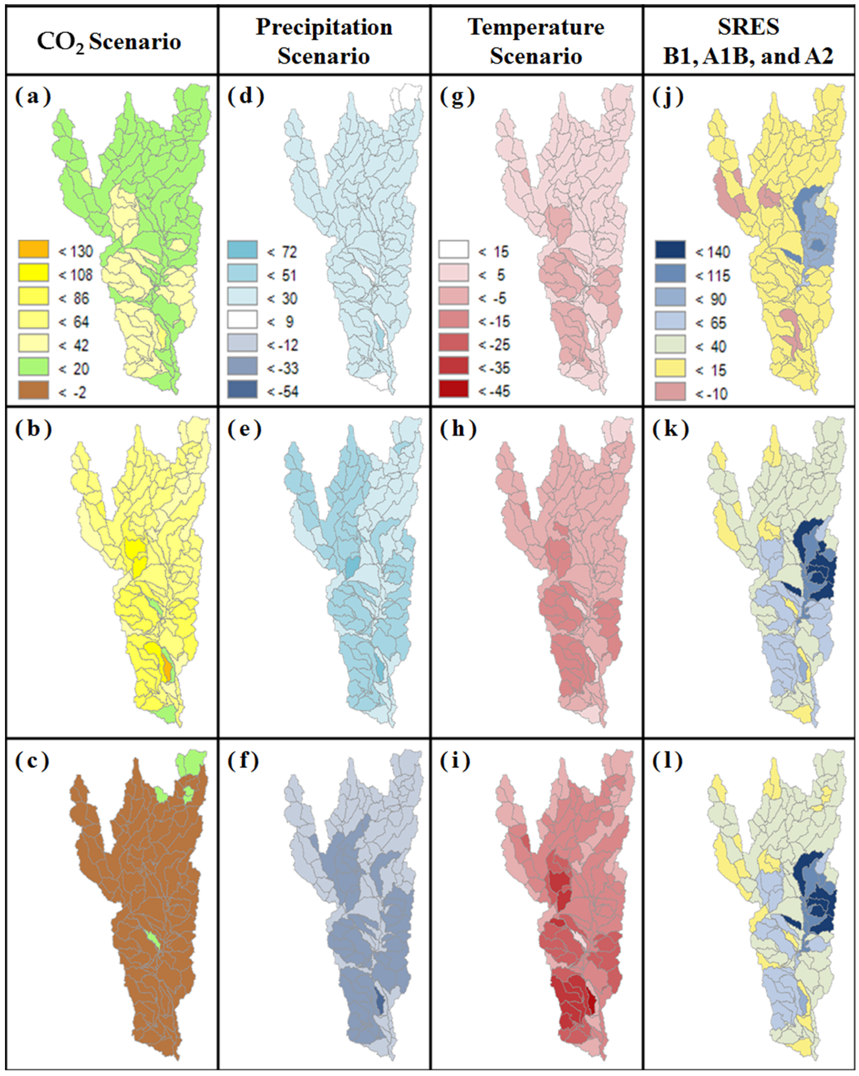
3.2.2. Precipitation

Scenarios 4 through 7 represent precipitation changes of +10%, +20%, −10%, and −20%, while holding the baseline CO2 concentration (330 ppm) and air temperature constant (Table 7). Annual average streamflow changes of 15.6%, 30%, −15.8, and −32.8% correspond to the changes implemented for the annual precipitation. On the other hand, changes in the annual average streamflow in the entire Chao Phraya River basin, 16.6%, 32.2%, −16.7%, and −34.5%, corresponded to the changes at Chai Nat Station. Figure 3d–f shows the spatial distributions of streamflow ratio of Scenarios 4 to 6, which reflect the results of the average streamflow changes. Figure 3f, which shows Scenario 6, represents the spatial distribution of the decrease in precipitation. It can be concluded that Scenario 7 will have a darker shade, signifying an overall decrease of streamflow ratio in the basin. Based on these results, streamflow and precipitation have a positive linear relationship. One of the significant factors that affect streamflow is soil water content. Figure 4 shows the plots of soil water content of different scenarios. Compared to the others, the precipitation scenarios have notable differences from the baseline; as precipitation was increased, the soil water content also steadily increased. Increases or decreases in precipitation directly lead to corresponding directional changes in the streamflow [88,89].
Figure 4. Water yield, soil water content, and groundwater recharge of Chao Phraya River basin under climate sensitivity scenarios.
Water 07 06665 g004
In terms of precipitation scenarios, the annual streamflow of Chao Phraya River have maximum changes of 35.9%, 70%, −7%, and −14.5%, and minimum changes of 5.9%, 11.6%, −37.3%, −71.4%. Figure 3g–i shows the variation of upstream flow, middle streamflow, and down streamflow from the Chao Phraya River. It can be seen that an increase in precipitation led to an increase in the annual average streamflow in the Chao Phraya Watershed, as indicated by Scenarios 4 and 5. These results coincide with other literature that investigated the hydrological impact of climate change and hydrological scenarios, which stated that the mean annual river discharge increases due to an increase in precipitation [90,91]. The decreased streamflow in Scenarios 6 and 7 also confirmed that precipitation plays a major role in streamflow variations.
During the wet season, a precipitation change was responsible for the streamflow variation [92]. In the upstream, the annual average streamflow was 249.2 m3/s in September, while the middle and down streams had around 562.8 m3/s and 671.8 m3/s, respectively. Figure 5 compares the seasonal variation of the peak streamflow for dry and wet seasons. The apparent increase in the streamflow in the increasing trend of the precipitation scenarios could lead to flooding events during the wet season. Monsoonal rains occur in the Chao Phraya River every year from May to October, making the watershed vulnerable to flood-related disasters during this season [93,94,95]. In this study, the streamflow increased in May and continued to rise until reaching their peak in September. The peak streamflow of the baseline and scenarios are highlighted in blue in Figure 5.
Figure 5. Seasonal variations of the peak stream flow under different climate scenarios in a year. The peak streamflow of each scenario is highlighted in blue to emphasize the difference from the baseline. It includes the upstream, middle stream, and downstream regions of the Chao Phraya River.
Water 07 06665 g005

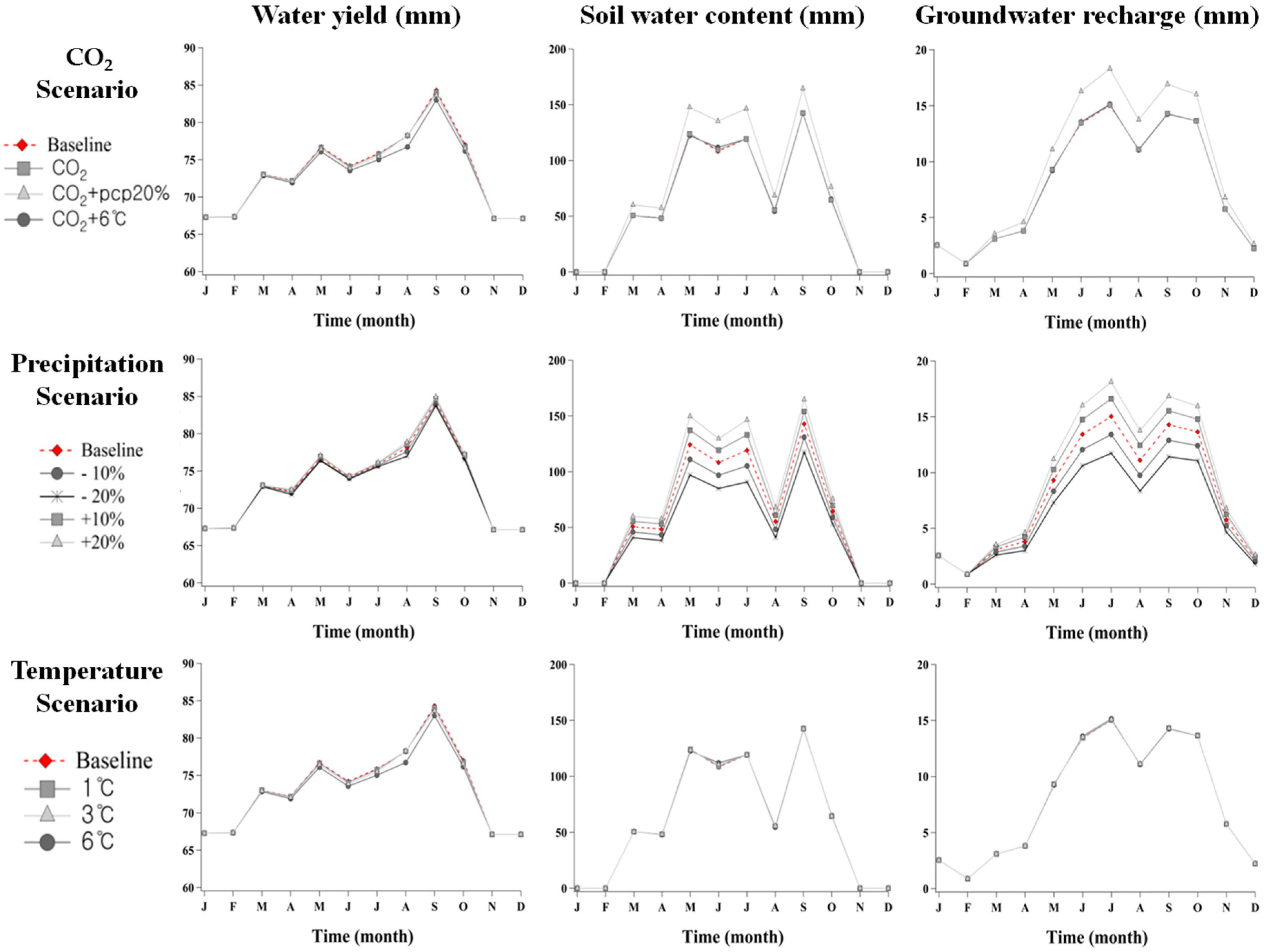
3.2.3. Air Temperature

Scenarios 8–10 represent air temperature increases of 1 °C, 3 °C, and 6 °C, respectively, from the baseline, while maintaining the CO2 concentration at 330 ppm with no change in precipitation. Table 7 shows the variation of streamflow at the Chai Nat Station, which decreased by −3.1%, −9.3%, and −19.2% for Scenarios 8, 9, and 10. The table also includes the annual average streamflow and maximum and minimum changes in the annual average streamflow of the whole basin for each scenario. It was found that as the temperature increases, the average streamflow significantly decreases. These results indicate that a rise in temperature due to global warming may lead to a serious water shortage [96].
These results are similar to the results of spatial variations of previous scenarios, such as Scenarios 3, 6, and 7, which either increased the temperature or decreased the precipitation. In Scenario 6, Figure 3f shows that the southern area has a more sensitive response due to the significant decrease in its streamflow level. The southern part of the Chao Phraya Watershed also represents Central Thailand, which is described as a lush, fertile valley. This area is a perfect catchment basin of the mountainous Northern Thailand; thus, a drastic decrease in the streamflow will be first noticed in this area then followed by the rest of the watershed [97]. Figure 3g–i also shows a decrease in streamflow change in the entire river basin.

3.2.4. Climate Change Effects of SRES

We applied downscaled GCM outputs to modify the meteorological data in the SWAT model to predict the hydrological effect of potential future climate for the mid-21st century. Figure 3j–l illustrates baseline conditions of the monthly average precipitation and air temperature for the baseline period (2003–2011). Future climate change scenarios under three greenhouse gas emission scenarios from 2050–2059 are then projected.
Figure 3j–l show the variation of locational streamflow under different emission scenarios. The predicted streamflow displayed a higher frequency of flood events, which was expected due to a shift in the peak flow runoff in early May. Relative to the baseline conditions, the annual average percentage changes of the projected climate scenarios in streamflow under B1, A1B, and A2 were 12.3%, 45.7%, and 40.8% respectively. The maximum values of annual average percentage changes were 95.7%, 138.3%, and 132.2%, whereas the minimum values were −33.3%, 5.3%, −0.7% in the basin. The variations in streamflow for the upstream, middle stream, and downstream follow similar baseline patterns under the projected climate scenarios.
The previous spatial streamflow variations of Scenarios 8 to 10 yielded a decrease in streamflow at the southern part of the basin, whereas the middle-eastern area had a more significant increase in percentage change of the streamflow when the projected climate change scenario under SRES was applied. The middle-eastern area represents Northeast Thailand, an arid region having a rolling surface and undulating hills that often experiences harsh climatic conditions. These results are justified, as Chinvanno [98] previously stated that this part of Thailand will experience a significant shift in season with increased rainfall and a longer late season rain peak, consequently increasing its water quantity. The streamflow variation of three emission scenarios commonly displayed an increase of streamflow in this area of the river basin.

4. Conclusions

The SWAT model was used to create a hydrological model of the Chao Phraya Watershed to investigate the effect of climate sensitivity and greenhouse gas emission scenarios on its streamflow. The model yielded percentage increases of the streamflow that revealed a need to create safety measures during flood events: daily average streamflow (72.3%), during the wet season in early May (22.7%), and after May (70.1%). This study also achieved its objectives.
  • The SWAT model showed a satisfactory performance in terms of calibration and validation, with R2 and NSE values greater than 0.5.
  • Precipitation scenarios yielded streamflow variations that corresponded to the change of rainfall intensity and amount of rainfall, while scenarios with increased air temperature yielded a decrease in water level leading to a water shortage. However, the three greenhouse gas emission scenarios from 2051–2059 had streamflow variations that increased from the baseline (2003–2011).
  • Scenarios 1 to 3 were related to an increase in CO2 concentration scenarios, which reduced stomatal conductance and increased the leaf area index. The results showed an increase in streamflow levels; however, a negative change in streamflow was also observed when the air temperature increased.
  • Variations under three SRES indicate low streamflow values compared to those of the southern Chao Phraya Watershed. Hence, flood measures should be performed in the main streamline of Chao Phraya River and the southern area of the basin. As such, further water resource management will be needed in the northeastern area of the Chao Phraya river basin in the future.
Further increasing the uncertainty of climate change brings a corresponding uncertainty into the predictions of severe flood and drought. In addition, change in the landuse of the Chao Phraya River subbasins may result in a different distribution, which also depends on the changes of climate conditions such as climate sensitivity scenarios and the three emission scenarios.

Acknowledgments

This project was partially funded by the Asia-Pacific Network for Global Change Research (APN) (ARCP2013-23NMY-Sthiannopkao) and by the Basic Science Research Program through the National Research Foundation (NRF) of Korea funded by the Ministry of Education (NRF-2014R1A1A2059680).

Author Contributions

Mayzonee Ligaray arranged and wrote the paper while Hanna Kim developed the methodology and built the SWAT model. Suthipong Sthiannopkao, Seungwon Lee, and Kyung Hwa Cho prepared the climate data. Joon Ha Kim made the overall conclusion.

Conflicts of Interest

The authors declare no conflict of interest.

References

  1. Graiprab, P.; Pongput, K.; Tangtham, N.; Gassman, P.W. Hydrologic evaluation and effect of climate change on the at Samat watershed, northeastern region, Thailand. Int. Agric. Eng. J. 2010, 19, 12–22. [Google Scholar]
  2. Immerzeel, W.W.; van Beek, L.P.H.; Bierkens, M.F.P. Climate change will affect the Asian water towers. Science 2010, 328, 1382–1385. [Google Scholar] [CrossRef] [PubMed]
  3. Kundzewicz, Z.W.; Mata, L.J.; Arnell, N.W.; DÖLl, P.; Jimenez, B.; Miller, K.; Oki, T.; ŞEn, Z.; Shiklomanov, I. The implications of projected climate change for freshwater resources and their management. Hydrol. Sci. J. 2008, 53, 3–10. [Google Scholar] [CrossRef]
  4. Tebaldi, C.; Smith, R.L.; Nychka, D.; Mearns, L.O. Quantifying uncertainty in projections of regional climate change: A bayesian approach to the analysis of multimodel ensembles. J. Clim. 2005, 18, 1524–1540. [Google Scholar] [CrossRef]
  5. Allen, M.R.; Stott, P.A.; Mitchell, J.F.B.; Schnur, R.; Delworth, T.L. Quantifying the uncertainty in forecasts of anthropogenic climate change. Nature 2000, 407, 617–620. [Google Scholar] [CrossRef] [PubMed]
  6. Le, T.; Sharif, H. Modeling the projected changes of river flow in central Vietnam under different climate change scenarios. Water 2015, 7, 3579–3598. [Google Scholar] [CrossRef]
  7. Kay, A.L.; Jones, R.G.; Reynard, N.S. Rcm rainfall for UK flood frequency estimation. II. Climate change results. J. Hydrol. 2006, 318, 163–172. [Google Scholar] [CrossRef]
  8. Delpla, I.; Jung, A.V.; Baures, E.; Clement, M.; Thomas, O. Impacts of climate change on surface water quality in relation to drinking water production. Environ. Int. 2009, 35, 1225–1233. [Google Scholar] [CrossRef] [PubMed]
  9. Wang, H.; Gao, J.E.; Zhang, M.J.; Li, X.H.; Zhang, S.L.; Jia, L.Z. Effects of rainfall intensity on groundwater recharge based on simulated rainfall experiments and a groundwater flow model. CATENA 2015, 127, 80–91. [Google Scholar] [CrossRef]
  10. Routschek, A.; Schmidt, J.; Kreienkamp, F. Impact of climate change on soil erosion—A high-resolution projection on catchment scale until 2100 in Saxony/Germany. CATENA 2014, 121, 99–109. [Google Scholar] [CrossRef]
  11. Nearing, M.A.; Jetten, V.; Baffaut, C.; Cerdan, O.; Couturier, A.; Hernandez, M.; le Bissonnais, Y.; Nichols, M.H.; Nunes, J.P.; Renschler, C.S.; et al. Modeling response of soil erosion and runoff to changes in precipitation and cover. CATENA 2005, 61, 131–154. [Google Scholar] [CrossRef]
  12. Wang, H.; Chen, L.; Yu, X. Distinguishing human and climate influences on streamflow changes in luan river basin in China. CATENA 2015, in press. [Google Scholar] [CrossRef]
  13. Wang, S.; Wang, Y.; Ran, L.; Su, T. Climatic and anthropogenic impacts on runoff changes in the songhua river basin over the last 56 years (1955–2010), Northeastern China. CATENA 2015, 127, 258–269. [Google Scholar] [CrossRef]
  14. Knox, J.C. Large increases in flood magnitude in response to modest changes in climate. Nature 1993, 361, 430–432. [Google Scholar] [CrossRef]
  15. Clarvis, M.H.; Fatichi, S.; Allan, A.; Fuhrer, J.; Stoffel, M.; Romerio, F.; Gaudard, L.; Burlando, P.; Beniston, M.; Xoplaki, E.; et al. Governing and managing water resources under changing hydro-climatic contexts: The case of the upper Rhone basin. Environ. Sci. Policy 2014, 43, 56–67. [Google Scholar] [CrossRef]
  16. Costanza, R.; Bohensky, E.; Butler, J.R.A.; Bohnet, I.; Delisle, A.; Fabricius, K.; Gooch, M.; Kubiszewski, I.; Lukacs, G.; Pert, P.; et al. A scenario analysis of climate change and ecosystem services for the Great Barrier Reef. In Treatise on Estuarine and Coastal Science; Wolanski, E., McLusky, D., Eds.; Academic Press: Waltham, MA, USA, 2011; pp. 305–326. [Google Scholar]
  17. López-Moreno, J.I.; Zabalza, J.; Vicente-Serrano, S.M.; Revuelto, J.; Gilaberte, M.; Azorin-Molina, C.; Morán-Tejeda, E.; García-Ruiz, J.M.; Tague, C. Impact of climate and land use change on water availability and reservoir management: Scenarios in the Upper Aragón river, Spanish Pyrenees. Sci. Total Environ. 2014, 493, 1222–1231. [Google Scholar] [CrossRef] [PubMed]
  18. Pingale, S.M.; Jat, M.K.; Khare, D. Integrated urban water management modelling under climate change scenarios. Resour. Conserv. Recycl. 2014, 83, 176–189. [Google Scholar] [CrossRef]
  19. Nam, W.H.; Choi, J.Y.; Hong, E.M. Irrigation vulnerability assessment on agricultural water supply risk for adaptive management of climate change in South Korea. Agric. Water Manag. 2015, 152, 173–187. [Google Scholar] [CrossRef]
  20. United Nations/World Water Assessment Programme. United Nations World Water Development Report: Water for People, Water for Life, 1st ed.; United Nations Educational, Scientific and Cultural Organization (UNESCO): Paris, France; Berghahn Books: Brooklyn, NY, USA, 2003. [Google Scholar]
  21. Asian Development Bank. The Economics of Climate Change in Southeast Asia: A Regional Review; Asian Development Bank: Metro Manila, Philippines, 2009. [Google Scholar]
  22. Chaturongkasumrit, Y.; Techaruvichit, P.; Takahashi, H.; Kimura, B.; Keeratipibul, S. Microbiological evaluation of water during the 2011 flood crisis in Thailand. Sci. Total Environ. 2013, 463–464, 959–967. [Google Scholar] [CrossRef] [PubMed]
  23. Vachiramon, V.; Busaracome, P.; Chongtrakool, P.; Puavilai, S. Skin diseases during floods in Thailand. J. Med. Assoc. Thail. 2008, 91, 479–484. [Google Scholar]
  24. Assanangkornchai, S.; Tangboonngam, S.; Edwards, S.G. The flooding of Hat Yai: Predictors of adverse emotional responses to a natural disaster. Stress Health 2004, 20, 81–89. [Google Scholar] [CrossRef]
  25. Nara, P.; Mao, G.G.; Yen, T.B. Climate change impacts on agricultural products in Thailand: A case study of thai rice at the Chao Phraya River basin. APCBEE Procedia 2014, 8, 136–140. [Google Scholar] [CrossRef]
  26. Ziegler, A.D.; Lim, H.; Tantasarin, C.; Jachowski, N.R.; Wasson, R. Floods, false hope, and the future. Hydrol. Process. 2012, 26, 1748–1750. [Google Scholar] [CrossRef]
  27. Komori, D.; Nakamura, S.; Kiguchi, M.; Nishijima, A.; Yamazaki, D.; Suzuki, S.; Kawasaki, A.; Oki, K.; Oki, T. Characteristics of the 2011 Chao Phraya River flood in central Thailand. Hydrol. Res. Lett. 2012, 6, 41–46. [Google Scholar] [CrossRef]
  28. Raungratanaamporn, I.S.; Pakdeeburee, P.; Kamiko, A.; Denpaiboon, C. Government-communities collaboration in disaster management activity: Investigation in the current flood disaster management policy in Thailand. Procedia Environ. Sci. 2014, 20, 658–667. [Google Scholar] [CrossRef]
  29. Thaipadungpanit, J.; Wuthiekanun, V.; Chantratita, N.; Yimsamran, S.; Amornchai, P.; Boonsilp, S.; Maneeboonyang, W.; Tharnpoophasiam, P.; Saiprom, N.; Mahakunkijcharoen, Y.; et al. Leptospira species in floodwater during the 2011 floods in the Bangkok Metropolitan Region, Thailand. Am. J. Trop. Med. Hyg. 2013, 89, 794–796. [Google Scholar] [CrossRef] [PubMed]
  30. Ngaosuwankul, N.; Thippornchai, N.; Yamashita, A.; Vargas, R.E.M.; Tunyong, W.; Mahakunkijchareon, Y.; Ikuta, K.; Singhasivanon, P.; Okabayashi, T.; Leaungwutiwong, P. Detection and characterization of enteric viruses in flood water from the 2011 Thai flood. Jpn. J. Infect. Dis. 2013, 66, 398–403. [Google Scholar] [CrossRef] [PubMed]
  31. Thepent, V. Agricultural Engineering and Technology for Food Security and Sustainable Agriculture in Thailand; Department of Agriculture Thailand: Bangkok Thailand, 2005. [Google Scholar]
  32. Molle, F.; Sutthi, C.; Keawkulaya, J.; Korpraditskul, R. Water management in raised bed systems: A case study from the Chao Phraya Delta, Thailand. Agric. Water Manag. 1999, 39, 1–17. [Google Scholar] [CrossRef]
  33. Teamsuwan, V.; Satoh, M. Comparative analysis of management of three water users’ organizations: Successful cases in the Chao Phraya Delta, Thailand. Paddy Water Environ. 2009, 7, 227–237. [Google Scholar] [CrossRef]
  34. Bossa, A.; Diekkrüger, B.; Agbossou, E. Scenario-based impacts of land use and climate change on land and water degradation from the meso to regional scale. Water 2014, 6, 3152–3181. [Google Scholar] [CrossRef]
  35. Malanson, G.P.; Verdery, A.M.; Walsh, S.J.; Sawangdee, Y.; Heumann, B.W.; McDaniel, P.M.; Frizzelle, B.G.; Williams, N.E.; Yao, X.; Entwisle, B.; et al. Changing crops in response to climate: Virtual nang rong, Thailand in an agent based simulation. Appl. Geogr. 2014, 53, 202–212. [Google Scholar] [CrossRef] [PubMed]
  36. Molle, F. Scales and power in river basin management: The Chao Phraya River in Thailand. Geogr. J. 2007, 173, 358–373. [Google Scholar] [CrossRef]
  37. World Water Assessment Programme. Water for People, Water for Life: A Joint Report by the Twenty-Three un Agencies Concerned with Freshwater; UNESCO Pub.: Paris, France, 2003. [Google Scholar]
  38. Bachelet, D.; Brown, D.; Böhm, M.; Russell, P. Climate change in Thailand and its potential impact on rice yield. Clim. Chang. 1992, 21, 347–366. [Google Scholar] [CrossRef]
  39. Arias, R.; Rodríguez-Blanco, M.; Taboada-Castro, M.; Nunes, J.; Keizer, J.; Taboada-Castro, M. Water resources response to changes in temperature, rainfall and CO2 concentration: A first approach in NW Spain. Water 2014, 6, 3049–3067. [Google Scholar] [CrossRef]
  40. Wu, Y.; Liu, S.; Gallant, A.L. Predicting impacts of increased CO2 and climate change on the water cycle and water quality in the semiarid james river basin of the midwestern USA. Sci. Total Environ. 2012, 430, 150–160. [Google Scholar] [CrossRef] [PubMed]
  41. Varanou, E.; Gkouvatsou, E.; Baltas, E.; Mimikou, M. Quantity and quality integrated catchment modeling under climate change with use of soil and water assessment tool model. J. Hydrol. Eng. 2002, 7, 228–244. [Google Scholar] [CrossRef]
  42. Stone, M.C.; Hotchkiss, R.H.; Hubbard, C.M.; Fontaine, T.A.; Mearns, L.O.; Arnold, J.G. Impacts of Climate Change on Missouri River Basin Water Yield; Wiley Online Library: Hoboken, NJ, USA, 2001. [Google Scholar]
  43. Zhang, X.; Srinivasan, R.; Hao, E. Predicting hydrologic response to climate change in the Luohe River basin using the SWAT model. Trans. ASABE 2007, 50, 901–910. [Google Scholar] [CrossRef]
  44. Ficklin, D.L.; Luo, Y.; Luedeling, E.; Zhang, M. Climate change sensitivity assessment of a highly agricultural watershed using SWAT. J. Hydrol. 2009, 374, 16–29. [Google Scholar] [CrossRef]
  45. Abbaspour, K.C.; Faramarzi, M.; Ghasemi, S.S.; Yang, H. Assessing the impact of climate change on water resources in Iran. Water Resour. Res. 2009, 45. [Google Scholar] [CrossRef]
  46. Hanratty, M.P.; Stefan, H.G. Simulating climate change effects in a minnesota agricultural watershed. J. Environ. Qual. 1998, 27, 1524–1532. [Google Scholar] [CrossRef]
  47. Gosain, A.; Rao, S.; Basuray, D. Climate change impact assessment on hydrology of Indian River basins. Curr. Sci. 2006, 90, 346–353. [Google Scholar]
  48. Githui, F.; Gitau, W.; Mutua, F.; Bauwens, W. Climate change impact on SWAT simulated streamflow in Western Kenya. Int. J. Climatol. 2009, 29, 1823–1834. [Google Scholar] [CrossRef]
  49. Jha, M.; Pan, Z.; Takle, E.S.; Gu, R. Impacts of climate change on streamflow in the upper Mississippi River basin: A regional climate model perspective. J. Geophys. Res. Atmos. 2004, 109. [Google Scholar] [CrossRef]
  50. Wang, S.; Kang, S.; Zhang, L.; Li, F. Modelling hydrological response to different land-use and climate change scenarios in the Zamu River basin of Northwest China. Hydrol. Process. 2008, 22, 2502–2510. [Google Scholar] [CrossRef]
  51. Fontaine, T.A.; Klassen, J.F.; Cruickshank, T.S.; Hotchkiss, R.H. Hydrological response to climate change in the black hills of south dakota, USA. Hydrol. Sci. J. 2001, 46, 27–40. [Google Scholar] [CrossRef]
  52. SRTM 90m Digital Elevation Data. Available online: http://srtm.csi.cgiar.org/ (accessed on 2 September 2015).
  53. Global Land Cover Characterization. Available online: http://edc2.usgs.gov/glcc/glcc.php (accessed on 2 September 2015).
  54. Leon, L.F. Step by step geo-processing and set-up of the required watershed data for MWSWAT (mapwindow SWAT). Available online: http://www.waterbase.org/docs/Geo_Process.pdf (accessed on 1 December 2015).
  55. Qiang, C.; Si, G.; Dayong, Q.; Zuhao, Z. Analysis of SWAT 2005 parameter sensitivity with LH-OAT method. HKIE Trans. 2010, 17, 1–7. [Google Scholar]
  56. McKay, M.D.; Beckman, R.J.; Conover, W.J. Comparison of three methods for selecting values of input variables in the analysis of output from a computer code. Technometrics 1979, 21, 239–245. [Google Scholar]
  57. Morris, M.D. Factorial sampling plans for preliminary computational experiments. Technometrics 1991, 33, 161–174. [Google Scholar] [CrossRef]
  58. Feng, G.; Sharratt, B. Sensitivity analysis of soil and PM10 loss in Weps using the LHS-OAT method. Trans. ASAE 2005, 48, 1409–1420. [Google Scholar] [CrossRef]
  59. Croitoru, A.E.; Minea, I. The impact of climate changes on rivers discharge in Eastern Romania. Theor. Appl. Clim. 2014, 1–11. [Google Scholar] [CrossRef]
  60. Grillakis, M.G.; Tsanis, I.K.; Koutroulis, A.G. Application of the HBV hydrological model in a flash flood case in Slovenia. Nat. Hazards Earth Syst. Sci. 2010, 10, 2713–2725. [Google Scholar] [CrossRef]
  61. Krause, P.; Boyle, D.; Bäse, F. Comparison of different efficiency criteria for hydrological model assessment. Adv. Geosci. 2005, 5, 89–97. [Google Scholar] [CrossRef]
  62. Moriasi, D.N.; Arnold, J.G.; van Liew, M.W.; Bingner, R.L.; Harmel, R.D.; Veith, T.L. Model evaluation guidelines for systematic quantification of accuracy in watershed simulations. Trans. Asabe 2007, 50, 885–900. [Google Scholar] [CrossRef]
  63. Mishra, A.; Kar, S. Modeling hydrologic processes and NPS pollution in a small watershed in subhumid subtropics using SWAT. J. Hydrol. Eng. 2011, 17, 445–454. [Google Scholar] [CrossRef]
  64. Gitau, M.W.; Chaubey, I. Regionalization of SWAT model parameters for use in ungauged watersheds. Water 2010, 2, 849–871. [Google Scholar] [CrossRef]
  65. Singh, J.; Knapp, H.V.; Arnold, J.G.; Demissie, M. Hydrlogical modeling of the Iroquois River watershed using HSPF and SWAT. J. Am. Water Resour. Assoc. 2005, 41, 343–360. [Google Scholar] [CrossRef]
  66. Setegn, S.G.; Melesse, A.M.; Haiduk, A.; Webber, D.; Wang, X.; McClain, M.E. Modeling hydrological variability of fresh water resources in the Rio Cobre watershed, Jamaica. CATENA 2014, 120, 81–90. [Google Scholar] [CrossRef]
  67. Chu, T.W.; Shirmohammadi, A.; Montas, H.; Sadeghi, A. Evaluation of the SWAT model's sediment and nutrient components in the Piedmont physiographic region of Maryland. Trans. Am. Soc. Agric. Eng. 2004, 47, 1523–1538. [Google Scholar] [CrossRef]
  68. Moriasi, D.; Arnold, J.; van Liew, M.; Bingner, R.; Harmel, R.; Veith, T. Model evaluation guidelines for systematic quantification of accuracy in watershed simulations. Trans. ASABE 2007, 50, 885–900. [Google Scholar] [CrossRef]
  69. Watson, R.T.; Zinyowera, M.C.; Moss, R.H. The Regional Impacts of Climate Change: An Assessment of Vulnerability; Cambridge University Press: Cambridge, UK, 1997. [Google Scholar]
  70. Dix, M.; Gordon, H. Csiro mk3.5 Climate System Model Output: Tasmanian Partnership for Advanced Computing; Centre for Australian Weather and Climate Research: Victoria, Australia, 2012. [Google Scholar]
  71. Watterson, I.; O’Farrell, S. Climate change simulated by full and mixed-layer ocean versions of CSIRO Mk3.5 and Mk3.0: Large-scale sensitivity. Asia Pac. J. Atmos. Sci. 2013, 49, 375–387. [Google Scholar] [CrossRef]
  72. Gordon, H.; O’Farrell, S.; Collier, M.; Dix, M.; Rotstayn, L.; Kowalczyk, E.; Hirst, T.; Watterson, I. The CSIRO Mk3.5 Climate Model; CAWCR Technical Report No. 21; Centre for Australian Weather and Climate Research: Victoria, Australia, 2010. [Google Scholar]
  73. Intergovernmental Panel on Climate Change (IPCC). Summary for Policymakers: Emission Scenarios; IPCC: Geneva, Switzerland, 2000. [Google Scholar]
  74. Girod, B.; Wiek, A.; Mieg, H.; Hulme, M. The evolution of the IPCC’s emissions scenarios. Environ. Sci. Policy 2009, 12, 103–118. [Google Scholar] [CrossRef]
  75. Chien, H.; Yeh, P.J.F.; Knouft, J.H. Modeling the potential impacts of climate change on streamflow in agricultural watersheds of the midwestern United States. J. Hydrol. 2013, 491, 73–88. [Google Scholar] [CrossRef]
  76. Ribalaygua, J.; Pino, M.R.; Pórtoles, J.; Roldán, E.; Gaitán, E.; Chinarro, D.; Torres, L. Climate change scenarios for temperature and precipitation in Aragón (Spain). Sci. Total Environ. 2013, 463–464, 1015–1030. [Google Scholar] [CrossRef] [PubMed]
  77. Gaffin, S.R.; Rosenzweig, C.; Xing, X.; Yetman, G. Downscaling and geo-spatial gridding of socio-economic projections from the ipcc special report on emissions scenarios (SRES). Glob. Environ. Chang. 2004, 14, 105–123. [Google Scholar] [CrossRef]
  78. Arnell, N.W.; Livermore, M.J.L.; Kovats, S.; Levy, P.E.; Nicholls, R.; Parry, M.L.; Gaffin, S.R. Climate and socio-economic scenarios for global-scale climate change impacts assessments: Characterising the SRES storylines. Glob. Environ. Chang. 2004, 14, 3–20. [Google Scholar] [CrossRef]
  79. Chen, J.; Brissette, F.P.; Leconte, R. Uncertainty of downscaling method in quantifying the impact of climate change on hydrology. J. Hydrol. 2011, 401, 190–202. [Google Scholar] [CrossRef]
  80. Schuol, J.; Abbaspour, K.C.; Srinivasan, R.; Yang, H. Estimation of freshwater availability in the West African sub-continent using the SWAT hydrologic model. J. Hydrol. 2008, 352, 30–49. [Google Scholar] [CrossRef]
  81. Lenhart, T.; Eckhardt, K.; Fohrer, N.; Frede, H.G. Comparison of two different approaches of sensitivity analysis. Phys. Chem. Earth A B C 2002, 27, 645–654. [Google Scholar] [CrossRef]
  82. Jarvis, P. The interpretation of the variations in leaf water potential and stomatal conductance found in canopies in the field. Philos. Trans. R. Soc. Lond. B Biol. Sci. 1976, 273, 593–610. [Google Scholar] [CrossRef]
  83. Morison, J.I.L. Intercellular CO2 concentration and stomatal response to CO2. In Stomatal Function; Zeiger, E., Farquhar, G.D., Cowan, O.R., Eds.; Stanford University Press: Redwood City, CA, USA, 1987; pp. 229–252. [Google Scholar]
  84. Li, F.; Kang, S.; Zhang, J. Interactive effects of elevated CO2, nitrogen and drought on leaf area, stomatal conductance, and evapotranspiration of wheat. Agric. Water Manag. 2004, 67, 221–233. [Google Scholar] [CrossRef]
  85. Bernacchi, C.J.; Kimball, B.A.; Quarles, D.R.; Long, S.P.; Ort, D.R. Decreases in stomatal conductance of soybean under open-air elevation of CO2 are closely coupled with decreases in ecosystem evapotranspiration. Plant Physiol. 2007, 143, 134–144. [Google Scholar] [CrossRef] [PubMed]
  86. Wigley, T.; Jones, P. Influences of precipitation changes and direct CO2 effects on streamflow. Nature 1985, 314, 149–152. [Google Scholar] [CrossRef]
  87. Eckhardt, K.; Ulbrich, U. Potential impacts of climate change on groundwater recharge and streamflow in a central European low mountain range. J. Hydrol. 2003, 284, 244–252. [Google Scholar] [CrossRef]
  88. Kiely, G. Climate change in ireland from precipitation and streamflow observations. Adv. Water Resour. 1999, 23, 141–151. [Google Scholar] [CrossRef]
  89. McCabe, G.J.; Wolock, D.M. A step increase in streamflow in the conterminous United States. Geophys. Res. Lett. 2002, 29. [Google Scholar] [CrossRef]
  90. Kure, S.; Tebakari, T. Hydrological impact of regional climate change in the Chao Phraya River basin, Thailand. Hydrol. Res. Lett. 2012, 6, 53–58. [Google Scholar] [CrossRef]
  91. Ogata, T.; Saavedra Valeriano, O.C.; Yoshimura, C.; Liengcharernsit, W.; Hirabayashi, Y. Past and future hydrological simulations of Chao Phraya River basin. J. Jpn. Soc. Civil Eng. Ser. B1 Hydraul. Eng. 2012, 68, 97–102. [Google Scholar] [CrossRef]
  92. Groisman, P.Y.; Knight, R.W.; Karl, T.R. Heavy precipitation and high streamflow in the contiguous United States: Trends in the twentieth century. Bull. Am. Meteorol. Soc. 2001, 82, 219–246. [Google Scholar] [CrossRef]
  93. Sayama, T.; Tatebe, Y.; Iwami, Y.; Tanaka, S. Hydrologic sensitivity of flood runoff and inundation: 2011 Thailand floods in the Chao Phraya River basin. Nat. Hazards Earth Syst. Sci. Discuss. 2014, 2, 7027–7059. [Google Scholar] [CrossRef]
  94. Lee, D.; Oh, B.; Kim, H.; Lee, S.; Chung, G. Comparison of the hydro-climatological characteristics for the extra-ordinary flood induced by tropical cyclone in the selected river basins. Trop.Cyclone Res. Rev. 2013, 2, 45–54. [Google Scholar]
  95. Tamagno, B. Recent floods in Southeast Asia. Geodate 2012, 25, 2. [Google Scholar] [CrossRef]
  96. Christensen, N.; Wood, A.; Voisin, N.; Lettenmaier, D.; Palmer, R. The effects of climate change on the hydrology and water resources of the Colorado River basin. Clim. Chang. 2004, 62, 337–363. [Google Scholar] [CrossRef]
  97. Arnell, N.W. Climate change and global water resources. Glob. Environ. Chang. 1999, 9, 31–49. [Google Scholar] [CrossRef]
  98. Chinvanno, S. Information for Sustainable Development in Light of Climate Change in Mekong River basin; Southeast Asia START Regional Centre: Bangkok, Thailand, 2004. [Google Scholar]

