An Amplification Model for the Regional Estimation of Extreme Rainfall within Orographic Areas in Campania Region (Italy)

Abstract

Orography strongly interacts with the atmospheric circulation, especially during frontal events, generating an enhanced spatial variability of the rainfall field. Regional models of extreme rainfall have to deal with these circumstances in order to provide good spatial estimation of the regionalized variable. We present a model for the regional estimation of the mean of the probability distribution of the annual daily rainfall maxima in a region (Campania, Southern Italy) with complex orography. In a recent work, we found that areas with enhanced variability of extreme rainfall, in the same region, correspond to a particular set of orographic objects, which had been classified through an automatic, GIS-based geomorphological procedure. Here, we propose an approach that considers the same orographic objects as building blocks for a regional model that is able to capture the amplification of extreme rainfall caused by orography. The regional model is then the product of a basic stationary random spatial process and an amplification factor, whose values are related to the topographic features of the orographic objects. This approach represents a step towards the improvement of the predictive ability of regional models of extreme rainfall within orographically complex areas.

1. Introduction

The interaction between atmospheric circulation and topography, especially during frontal events, produces a significant increase of the precipitation amount in orographic areas [1,2]. This complex interaction also leads to an enhanced spatial rainfall variability [3,4,5,6]: this, associated with an inadequate and uneven rain-gauge network in mountainous areas, makes the observation and modeling of orographic effects a challenging task.

Here, we focus on the effect of orography on long-term probabilistic prediction of extreme rainfall at regional scale; hence, the main issue is to identify and model the effects induced by the orography over some statistical parameters of the rainfall extremes (in this work, annual daily rainfall maxima). Higher order statistical parameters are often considered either constant or smoothly varying over relatively large areas: this is a result of the sample estimation errors that usually mask spatial variability. On the contrary, estimates of low order statistical parameters, as the mean of the distribution, are less affected by sample errors and require a more accurate spatial model for regional estimation. Such statistical parameters of the annual maxima are affected by a multitude of events, with different characteristics. Physically based, meteorological models, although continuously improving, are storm-based models, therefore they are not suitable for the scope: the influence of orography needs to be embedded into the regionalization model of the parameters of the probability distribution of the rainfall extremes [7].

A common solution to the problem is to split the region into homogeneous sub-regions in order to apply regression relationships with at site descriptors of topography within the homogeneous regions [3,8,9,10]. A more sophisticated approach consists in coupling a regression model with a spatial, nonparametric model of the residuals [4,6,11].

Following the latter approach, topographic variables need to be included into the spatial interpolation methods used to map the statistical parameters of the rainfall maxima distribution. Interpolation methods, even as sophisticated as geostatistical techniques, can indeed still suffer from lack of rainfall data in mountainous areas, providing inaccurate and sometimes biased estimation of the regionalized variables in those areas.

In scientific literature, many regional studies deal with the estimation of rainfall in orographic areas using advanced kriging techniques that incorporate auxiliary topographic variables into the spatial interpolation model [3,4,6,11,12,13].

These methods may be categorized into two groups. One includes the methods that consider the external information directly in the kriging system, such as the kriging with an external drift or cokriging. The other consists of methods that first deal with the external information, for example by fitting a regression among the field and the external variables, and then apply an interpolation procedure, typically based on kriging, to the residuals. These methods are often referred to as “detrended kriging” [4].

This approach represent a significant improvement over simple regression analysis, and gives results whose quality depends on the physical meaning and complexity of the topographic descriptors and of the regression model. However, all these methods introduce local or locally averaged descriptors of the topographic surface as external variables for the orographic effects modeling. These descriptors are generally obtained through more or less complex elaboration of Digital Elevation Models (DEM): thus, they are not based on the identification of “orographic object” but only on local properties of the topography.

This approach to regional modeling of extreme rainfall can be improved by introducing an objective description and identification of orographic features [7,14]. This allows dividing the region into “topographically” homogeneous areas, for which different spatial rainfall variability is considered. This is what we basically want to show.

In Section 2, we present the study area, the available rainfall data and the current approach for the regional modeling of extreme rainfall as well as findings from previous works on the study area related to the influence of orography over the parameters of the probability distribution of the rainfall extremes. In Section 3, we define all the methods and models adopted. Finally, in Section 4 the results of the application of the proposed model for the regional estimation of the mean of the probability distribution of the annual daily rainfall maxima in the study area.

2. Study Area, Data and Previous Works

2.1. Description of the Study Area

The study area is the Campania region and some surroundings, in Southern Italy (Figure 1), located between the Apennines and the Tyrrhenian Sea.

The region is characterized by Mediterranean climate, with dry summers and wet winters. The mean annual precipitation ranges from 800 to 1100 mm/year.

The precipitations are largely generated by wet air masses that come predominantly from the Tyrrhenian Sea (i.e., southwest-northeast direction) and they are strongly influenced by the interaction with orography [15,16].

Figure 1 shows the location of the region and its terrain elevations by DEM.

Figure 1. Location of Campania region with DEM.

Figure 1. Location of Campania region with DEM.

The area is characterized by a complex topography (Figure 1), which Cuomo et al. [14] schematized through an automatic, objective, Geographical Information System (GIS)-based geomorphological procedure. This procedure identifies orographic entities by means of topographic concepts of key contour, key saddle, summit point and prominence (Figure 2).

Figure 2. Identification of the orographic entities. Reproduced with permission from Cuomo, A.; Guida, D.; Palmieri, V., J. Maps; Published by Taylor & Francis, 2011 [14].

Figure 2. Identification of the orographic entities. Reproduced with permission from Cuomo, A.; Guida, D.; Palmieri, V., J. Maps; Published by Taylor & Francis, 2011 [14].

The study in [14] provides orographic entities, hierarchically organized in nested orographic classes. Based on the results of a recent study [7], we have considered groups (4th order) and systems (3rd order) as meaningful objects for the regionalization study here presented (Figure 3).

Table 1 provides the extent of the selected orographic objects within the study area compared to its total extension.

Table 1. Extent of the study area and of the orographic areas (4th and 3rd order).

Areas	Area (km2)
Study area	18547
Orographic areas	5235

Table 1. Extent of the study area and of the orographic areas (4th and 3rd order).

Areas	Area (km2)
Study area	18547
Orographic areas	5235

2.2. Rainfall Data

The rainfall database comes from the VAPI (VAlutazione delle PIene, Flood Estimation) project [9,10], a national project for the regional analysis of the frequency of extreme rainfall and river floods, redacted within the National Research Council (CNR, Consiglio Nazionale delle Ricerche).

In Figure 3, the map of the region is presented along with the location of the 605 rain-gauges used for the analysis, among which 245 are placed in the region of interest. Besides the rain gauges located in the study area, we considered a convenient number of gauges in the surrounding area in order to avoid the presence of border errors in the spatial analysis.

In this work, we use the annual maxima of daily rainfall because they represent the most reliable and largely available data in the region. The length of the time series varies from 5 to 77 years, collected from the beginning of the last century until the year 2000, and it is on average equal to 45 years. The maximum value of the mean of the annual maxima of daily rainfall is 134.7 mm, the minimum is 39.3 mm, the average is 69.8 mm. The average coefficient of variation, C_v, is 0.353 and the average coefficient of skewness is 1.254.

Figure 3. Location of the study area with the rain gauges (triangles), the “anomalous” rain gauges (squares) (Section 2.3.2 and [7]) and the orographic barriers (solid grey) [14].

Figure 3. Location of the study area with the rain gauges (triangles), the “anomalous” rain gauges (squares) (Section 2.3.2 and [7]) and the orographic barriers (solid grey) [14].

2.3. Findings from Previous Works on the Study Area

2.3.1. The VAPI Model for Extreme Rainfall in the Region

The most recent and complete analysis of extreme rainfall at a regional scale for the study area was conducted within the VAPI national project [10] and described in the VAPI Campania regional report [9].

The VAPI procedure is based on the use of TCEV (Two Components Extreme Value, [17]) as a parent probabilistic model for the annual maxima of daily and sub-daily rainfall. The probabilistic model is coupled with a three level hierarchical procedure for the regional estimation of the parameters. The regional model is a simple model of homogeneous region at each level [8].

The first and second levels of regionalization deal with the regional estimation of the shape and scale parameters of the distribution. At both levels, the whole region can be considered homogeneous, with the shape and scale parameters that assume unique values everywhere.

At the third level, the regionalized variable is the mean of the annual maxima of daily (and hourly) rainfall. Here we report only the results for daily rainfall, which are the data analyzed in our work.

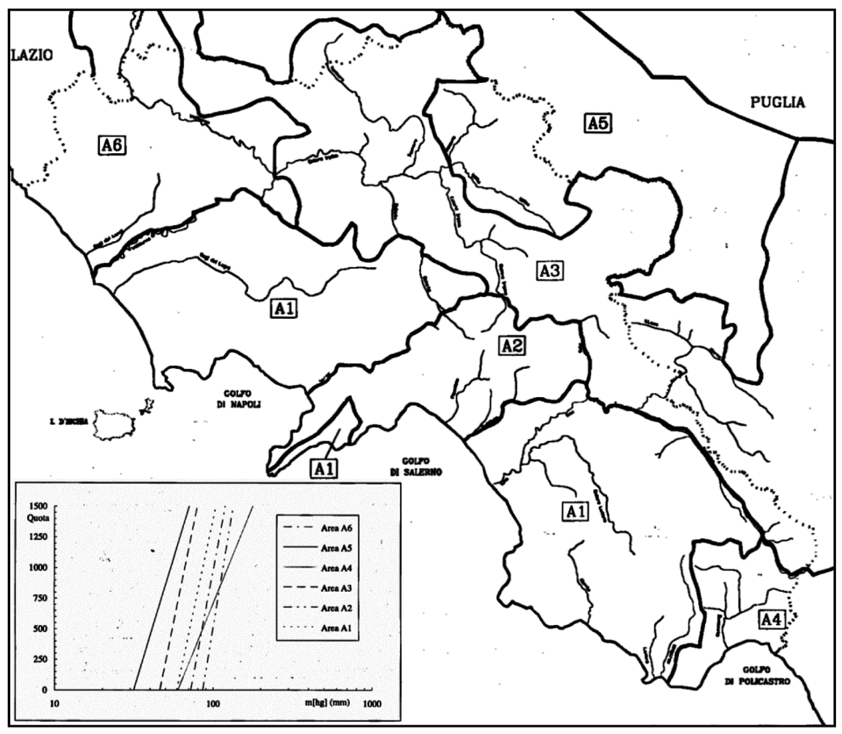
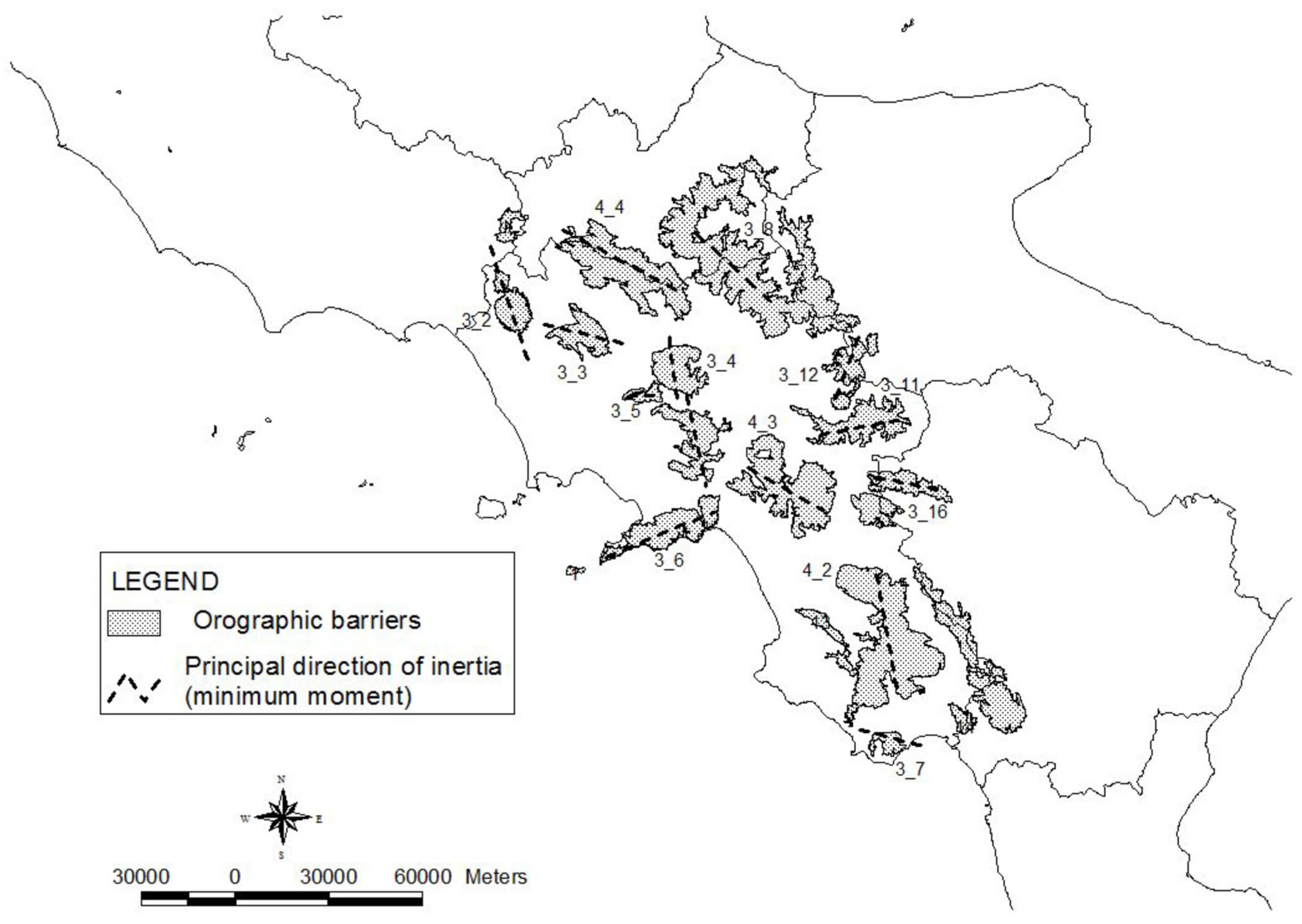
The regional analysis conducted within the VAPI project led to the identification of six homogeneous sub-regions at the third level. In each sub-region, a linear relationship between elevation and logarithm of mean annual daily rainfall maxima was estimated through a regression analysis.

The boundary of the homogeneous sub-regions are represented in Figure 4 along with the lines representing the six linear regressions that were fitted.

Figure 4. Map of the six homogeneous sub-regions for the mean annual daily rainfall maxima and linear relationships with elevation from VAPI Campania report. Reproduced with permission from Rossi, F. et al. Valutazione Delle Piene in Campania; Published by CNR-GNDCI, 1995 [9].

Figure 4. Map of the six homogeneous sub-regions for the mean annual daily rainfall maxima and linear relationships with elevation from VAPI Campania report. Reproduced with permission from Rossi, F. et al. Valutazione Delle Piene in Campania; Published by CNR-GNDCI, 1995 [9].

2.3.2. Identification of Spatial Outliers in Extreme Rainfall

In a recent work, we identified areas with enhanced spatial variability of the mean of the annual daily rainfall maxima through an innovative statistical procedure [7]. The procedure demonstrates how linear geostatistics is not able to capture the spatial variability of the regionalized variable in areas with a strong orographic forcing. It is an iterative statistical procedure applied to the logarithmic transformation of the original series of the annual daily rainfall maxima. The logarithmic transform was applied in order to obtain an approximately Gaussian field, for which linear geostatistics works the best.

Let Y(x) be the mean of the annual maxima of daily rainfall, Z(x) denote its logarithmic transformation as follows:

$$Z\text{(}x\text{)}=\ln Y\text{(}x\text{)}$$

(1)

The detection of the spatial non linearity, where the term “non-linearity” is used to characterize areas where linear geostatistics fails, due to an enhanced small scale variability of the field Z(x) was performed by analyzing the residuals of a cross-validation procedure in an innovative way.

The Kriging with Uncertain data (KUD) [18] estimator was run for the jack-knife estimation of the field in all the sampling points and then the standardized cross-validation residuals were calculated as follows:

$$e_i=\frac{Z\left(x_i\right)-{\widehat{Z}}_{JN}\left(x_i\right)}{{\sigma }_{JN}\left(x_i\right)}$$

(2)

where $Z\left(x_i\right)$ is the observed value of the field at sampling sites x_i, ${\widehat{Z}}_{JN}\left(x_i\right)$ is the jackknife KUD estimation of the field at sampling sites x_i and ${\sigma }_{JN}\left(x_i\right)$ denotes the estimated predictor variance (for theoretical details, refer to [7]).

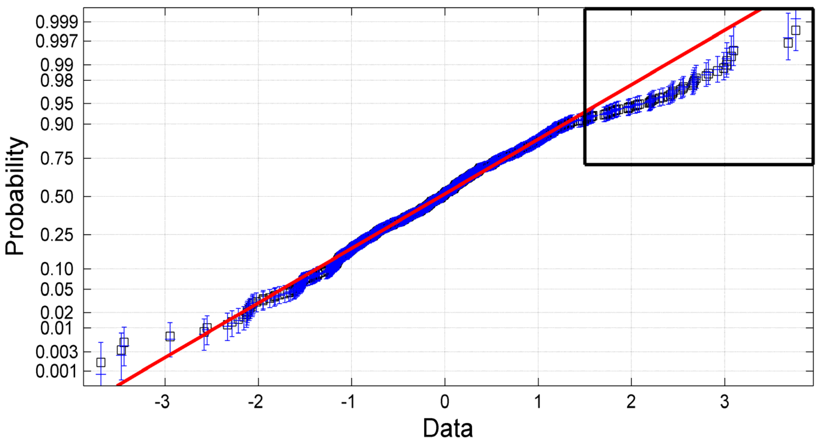
The cross-validation residual at a given sampling site, as defined in Equation (2), represents the sum of the interpolation and the sampling errors at that site. Under the hypotheses of the kriging predictor, the standardized cross-validation residuals should follow a standardized Gaussian distribution. Because of the orographic effects, instead, there are “anomalous” errors in some gauges. The “anomalous” errors can be identified as outliers on the upper tail of the error probability distribution in the Normal Probability Chart, which facilitates the comparison between the empirical and the expected theoretical distribution of the residuals. We considered as outliers the residuals whose 95% confidence interval (in blue in Figure 5) deviates from the straight line (in red in Figure 5), which represents the theoretical distribution (i.e., standardized Gaussian distribution) of the residuals on the Normal Probability Chart (Figure 5). Hereinafter, we refer to these sampling sites/rain gauges where the outliers occur as “anomalous” sites/rain gauges or as spatial outliers. In these sites, the kriging predictor fails with an unacceptable underestimation of the field.

Figure 5. Normal Probability Plot of the standardized residuals from cross-validation. Reproduced with permission from Furcolo, P.; Pelosi, A.; Rossi, F. Statistical identification of orographic effects in the regional analysis of extreme rainfall. Hydrol. Process. 2015 [7].

Figure 5. Normal Probability Plot of the standardized residuals from cross-validation. Reproduced with permission from Furcolo, P.; Pelosi, A.; Rossi, F. Statistical identification of orographic effects in the regional analysis of extreme rainfall. Hydrol. Process. 2015 [7].

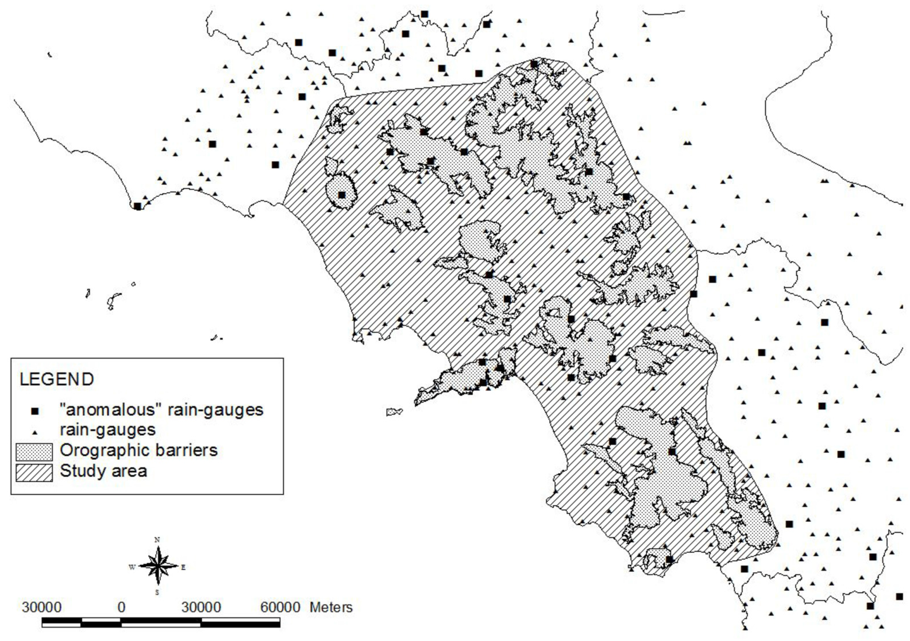
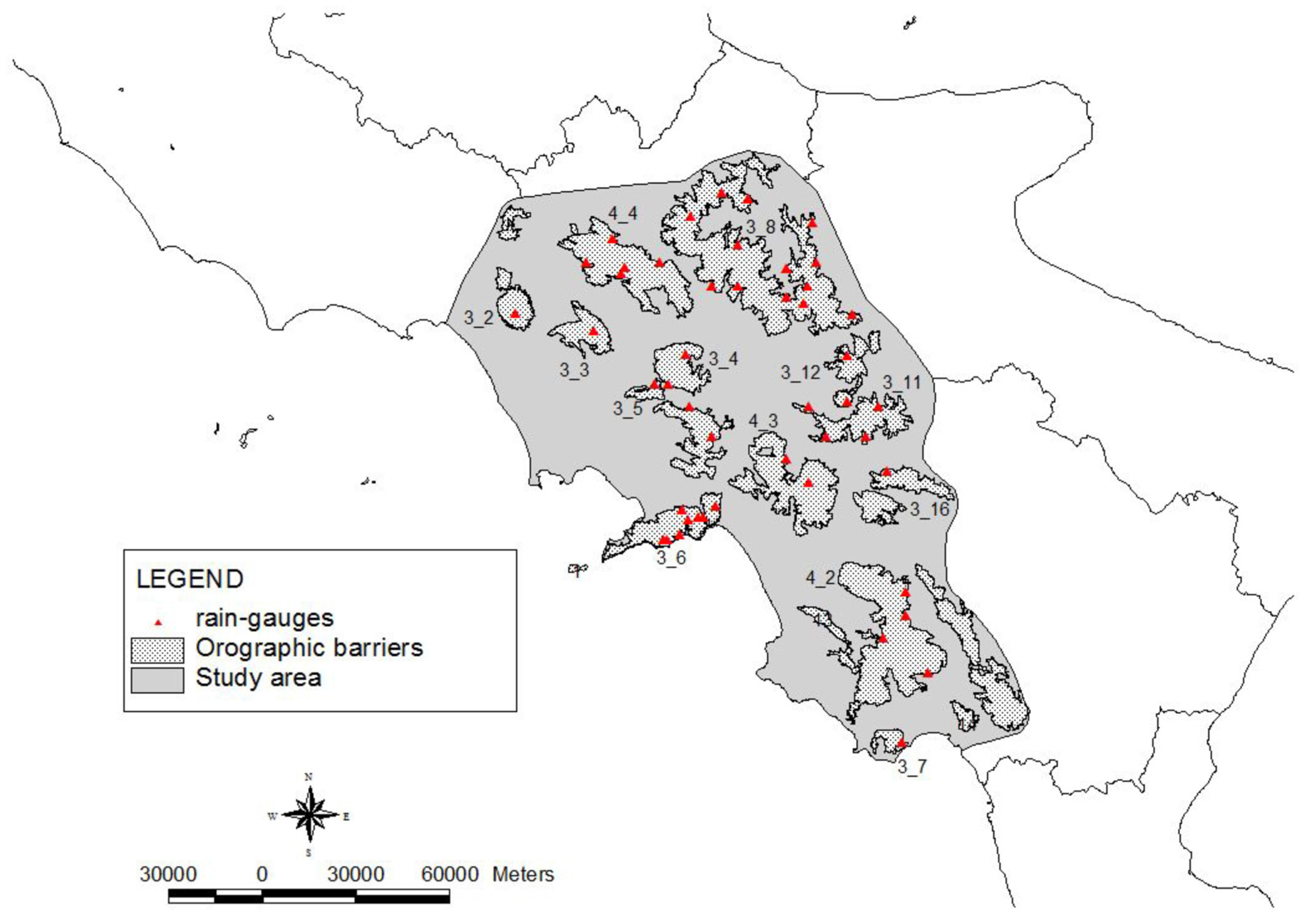
Figure 5 displays the Normal Probability Chart of the standardized residuals. In the upper tail of the distribution, within the black square, there are the anomalous errors, which significantly deviate from the theoretical distribution. These errors correspond to rain gauges marked as anomalous in Figure 3.

The statistical procedure detected the presence of 19 spatial outliers in the study area. The following step was to interpret the nature of these spatial outliers and highlight the physical factors that influence the rainfall field in such a way to produce a rainfall amplification that is so evident in the mean of the annual maxima.

In Table 2, we show some basic statistics of the data (i.e., annual daily rainfall maxima) in the study area, discerning between the anomalous subset and the remaining rain gauges. These statistics reveal that the average value of the field over the region (i.e., the average mean) is much higher in the anomalous gauges than in the other gauges of the region while the other statistics (i.e., average coefficient of variation, C_v, and average skewness) do not change as much. In particular, the circumstance that the skewness does not increase for the anomalous subset suggests that the mean is not affected by the presence of a few very intense events in the series but there is a more general amplification of the events producing the annual maximum.

Table 2. Statistics of the data in the study area, with distinction among the whole dataset, the anomalous subset and the remaining rain gauges [7].

Set of Rain Gauges	Number of Rain Gauges	Average Mean (mm)	Average Cv	Average Skewness
ALL	245	69.8	0.353	1.254
ANOMALOUS	19	101.5	0.382	1.229
NON ANOMALOUS	226	67.1	0.351	1.256

Table 2. Statistics of the data in the study area, with distinction among the whole dataset, the anomalous subset and the remaining rain gauges [7].

Set of Rain Gauges	Number of Rain Gauges	Average Mean (mm)	Average Cv	Average Skewness
ALL	245	69.8	0.353	1.254
ANOMALOUS	19	101.5	0.382	1.229
NON ANOMALOUS	226	67.1	0.351	1.256

In a climatologically homogeneous region like the one analyzed, orography may be identified as the main characteristic that may cause this amplification of the events producing the annual maxima. This is confirmed by a first examination of the results by comparing the anomalous rain gauges placed in the study area with the location of the orographic areas defined in Section 2.

The results of the comparison are interesting (see Table 3 for the details):

▪

The anomalous sites are located very close to orographic barriers: about 70% of the anomalous rain gauges are placed in orographic areas whereas only less than 20% of the gauges are located in those areas.

▪

About 30% of the rain gauges placed in orographic areas are anomalous, against 3% of anomalous gauges in the other areas.

Table 3. Main statistics referred to the location of the “anomalous” rain gauges.

Areas	Number of Rain Gauges	Number of Anomalous Rain Gauges	%
Study area	245	19	7.76
Orographic areas	47	13	27.7
%	19.2	68.4	–

Table 3. Main statistics referred to the location of the “anomalous” rain gauges.

Areas	Number of Rain Gauges	Number of Anomalous Rain Gauges	%
Study area	245	19	7.76
Orographic areas	47	13	27.7
%	19.2	68.4	–

3. Methods

3.1. Formulation of the Regional Model for the Mean of the Annual Daily Rainfall Maxima

The outcomes reported in the previous Section confirm the potential value of an approach based on the identification of orographic objects for the improvement of regional models of extreme rainfall. Here, we introduce a preliminary model for the regional estimation of the mean of the probability distribution of the annual daily rainfall maxima that gives a better interpretation of variability of the rainfall field in orographic areas. Despite its simplicity, this model is already very effective in increasing the accuracy of the regional estimates of the selected parameter.

We suppose that the mean of the annual maxima of daily rainfall, Y(x), can be seen as the product of a basic, weakly stationary process, Y’(x), and of an amplification factor, AF, that arises only in orographic areas:

$$Y(x)=AF\cdot Y\prime (\text{x})$$

(3)

Then, by taking the logarithm:

$$Z(x)=Z\prime (x)+\ln (AF)$$

(4)

The basic, weakly stationary process, or, better its logarithm, Z’(x), can be computed by using classic linear spatial interpolation techniques, such as KUD from the rainfall measurements in the valleys and in the plains.

The Amplification Factor, AF, corrects the linear estimations where it is necessary, i.e., in orographic areas as highlighted in Section 2. The Amplification Factor is computed accordingly an Amplification model (Section 3.2).

3.2. The Amplification Model

Here, we propose a model for the assessment of AF by relating its values to some global features of the orographic barriers. In the following, a set of topographic indices are evaluated for the estimation of AF in orographic areas.

3.2.1. Computation of Topographic Indices

Each isolated orographic object in the study area (Figure 3) has been treated as a unique homogeneous shape, for which a set of topographic indices has been computed, by means of a DEM having a spatial resolution of 20 m (Figure 1).

We considered five topographic indices that are representative of the process of orographic interaction and amplification of extreme rainfall [1,4]:

(i)

Mean slope, denoted as Sl (%), which is strictly related to the rate of climb of the wet air masses in proximity to the orographic object.

(ii)

Average elevation, z_mean (m a.s.l.), which is representative of the force, which leads up masses over orographic obstacles.

(iii)

Maximum elevation, z_max (m a.s.l.), which could state the intensity of the force, which leads up masses over orographic obstacles.

(iv)

Prominence, P (m), defined as the difference between the maximum elevation within the shape, z_max, and the average elevation of its perimeter line. It could express the presence of orographic obstacles in relation to the neighborhood.

(v)

Exposition, cosφ, defined as the cosine of the angle between the dominant direction of the wet air masses and the principal direction of inertia of each orographic object, related to the minimum moment of inertia (Figure 6).

We believe that the principal direction of inertia related to the minimum moment of inertia can conveniently represent the orientation of the orographic object itself.

In the Tyrrhenian area, the dominant direction of the wet air masses is known to be the direction southwest–northeast, which is inclined about 45° above the horizontal (west–east) line. In this case, a further statistical assessment have been done: We defined the dominant direction as the reference direction for measuring the angle φ, such that the linear correlation between ln(AF) and cosφ is maximum. The result was a dominant direction with inclination 41° above the horizontal (Figure 6), which is in good agreement with the fact that rainfall events in this area prevalently come from the southwest quadrant.

Exposition is important because it affects the dynamic of the interaction between the orographic obstacles and the wet air masses.

Figure 6 shows the orographic objects and their orientation by means of the principal directions of inertia related to the minimum moment.

Figure 6. Principal directions of inertia related to the minimum moment of the orographic object.

Figure 6. Principal directions of inertia related to the minimum moment of the orographic object.

3.2.2. Computation of AF

In our model, the Amplification Factor arises only in orographic areas, so that outside orographic areas its value is equal to the unity. Inside orographic areas, Equations (3) and (4) are useful for its evaluation, so that the logarithm of AF can be computed as the difference between the observed value Z(x_i) and the value Z′(x_i) estimated by the Kriging with Uncertain Data predictor using only the rainfall measurements in the valleys and in the plains, as follows:

$$\ln (AF)=\{\begin{array}{l}0\text{\hspace{1em}\hspace{1em}\hspace{1em}\hspace{1em}\hspace{1em} outside\hspace{0.17em}orographic\hspace{0.17em}areas}\\ Z(x)-Z\prime (x)\text{\hspace{0.17em}\hspace{0.17em}inside\hspace{0.17em}orographic\hspace{0.17em}areas}\end{array}$$

(5)

By means of Equation (5), we evaluated ln(AF) in each one of the 47 rain gauges, placed in orographic areas (Figure 7) and, then, we assigned to each orographic object a representative value of ln(AF), evaluated through the arithmetic mean of the values of ln(AF) related to the rain gauges within the object.

3.2.3. Regression Analysis

In our model, the values of the Amplification Factor (Section 3) are simply related to some global features of the orographic barriers, expressed by means of some more significant topographical indices (Section 3.2). This choice is mainly driven by the limited availability of rainfall data in these areas.

Univariate regressions between the Amplification Factor and the various topographical indices were first carried out. Then multiple regression analysis was performed.

Criteria to be respected are that the explanatory variables should not be highly correlated and they should represent physical explanations for AF variations.

The regression analysis has been performed using the data recorded in all 47 rain gauges (not just the anomalous ones) placed in orographic areas (Figure 7).

Figure 7. Rain gauges in orographic areas. The orographic shapes are numbered with two digits: the first one denotes the order (groups, 4th order, and systems, 3rd order), the second one identifies progressively the object.

Figure 7. Rain gauges in orographic areas. The orographic shapes are numbered with two digits: the first one denotes the order (groups, 4th order, and systems, 3rd order), the second one identifies progressively the object.

In particular, to proper select a combination of topographic indices and build the Amplification model by means of an eventually multivariate regression, we evaluated all the possible combinations of topographic indices, X_i, considering both a two-variate model and a three-variate model, as follows:

$$\ln (AF)=a_0+a_1\cdot X_1+a_2\cdot X_2$$

(6a)

$$\ln (AF)=a_0+a_1\cdot X_1+a_2\cdot X_2+a_3\cdot X_3$$

(6b)

The best combinations were found considering both the coefficient of determination, R², and the adjusted R², R²_adj, which allows to take account of the circumstance that R² automatically and spuriously increases when extra explanatory variables are added to the model. R²_adj was computed as follows:

$$R_{adj}^2=1-\frac{n-p}{n-p-1}\left(1-R^2\right)$$

(7)

where p is the total number of explanatory variables (i.e., topographic indices) in the model (not including the constant term), and n is the sample size.

Unlike R², the adjusted R² increases only when the increase in R², due to the inclusion of a new explanatory variable, is more than one would expect to see by chance.

4. Results and Discussion

In this Section, we firstly report the results of the regression analysis for the definition of the Amplification model. Then, we illustrate the results related to the application of the complete regional model for the estimation of the mean of the annual daily rainfall maxima to the study area by comparing its final performances against the actual regional model (i.e., VAPI) and a pure geostatistical interpolation.

4.1. The Amplification Model

Here, we considered each orographic object in the study area as a unique homogeneous shape for which we computed some topographic indices and the average value of ln(AF) (as stated in Section 3). Table 4 shows these values for the 14 orographic objects in the study area (numbered as in Figure 7).

Table 4. Values of ln(AF) and topographic indices for each orographic object.

ID Object	Ln(AF)	cosφ	Sl (%)	P (m)	zmean (m a.s.l.)	zmax (m a.s.l.)
3_2	0.210	0.390	0.267	700	481	1000
3_3	0.154	0.578	0.322	774	403	975
3_4	0.012	0.549	0.340	1080	649	1385
3_5	0.184	0.775	0.355	459	452	761
3_6	0.189	0.947	0.498	1234	1416	1429
3_7	0.323	0.563	0.389	825	937	1225
3_8	0.065	0.348	0.166	541	742	1128
3_11	−0.044	0.870	0.389	302	789	1003
3_12	0.093	0.885	0.189	438	759	1109
3_16	0.019	0.609	0.233	509	1034	1407
4_1	0.381	0.483	0.415	1092	774	1589
4_2	0.073	0.516	0.366	1299	966	1898
4_3	0.211	0.326	0.451	1117	1025	1813
4_4	0.294	0.351	0.347	1248	1115	2038

Table 4. Values of ln(AF) and topographic indices for each orographic object.

ID Object	Ln(AF)	cosφ	Sl (%)	P (m)	zmean (m a.s.l.)	zmax (m a.s.l.)
3_2	0.210	0.390	0.267	700	481	1000
3_3	0.154	0.578	0.322	774	403	975
3_4	0.012	0.549	0.340	1080	649	1385
3_5	0.184	0.775	0.355	459	452	761
3_6	0.189	0.947	0.498	1234	1416	1429
3_7	0.323	0.563	0.389	825	937	1225
3_8	0.065	0.348	0.166	541	742	1128
3_11	−0.044	0.870	0.389	302	789	1003
3_12	0.093	0.885	0.189	438	759	1109
3_16	0.019	0.609	0.233	509	1034	1407
4_1	0.381	0.483	0.415	1092	774	1589
4_2	0.073	0.516	0.366	1299	966	1898
4_3	0.211	0.326	0.451	1117	1025	1813
4_4	0.294	0.351	0.347	1248	1115	2038

The former step toward the regression analysis was to look at the correlation matrix to investigate at the same time the dependence between the multiple variables involved in the analysis. As we can see, from Table 5, the variables are all correlated to each other: the correlation between some topographic variables, such as exposition and slope or exposition and prominence is strictly related to the geological process that led to the formation of the orography itself. The correlation between prominence and slope, prominence and z_mean, prominence and z_max is instead mainly related to the definition itself of the prominence (Section 3.2) so that, as expected, the highest correlations are between P and these variables.

Table 5. Correlation matrix.

Variable	Ln(AF)	cosφ	Sl	P	zmean	zmax
ln(AF)	1	−0.332	0.397	0.450	0.117	0.269
(R2)	(1)	(0.110)	(0.158)	(0.203)	(0.014)	(0.072)
cosφ	−0.332	1	0.158	−0.368	0.113	−0.451
Sl	0.397	0.158	1	0.589	0.429	0.355
P	0.450	−0.368	0.589	1	0.502	0.809
zmean	0.117	0.113	0.429	0.502	1	0.671
zmax	0.269	−0.451	0.355	0.809	0.671	1

Table 5. Correlation matrix.

Variable	Ln(AF)	cosφ	Sl	P	zmean	zmax
ln(AF)	1	−0.332	0.397	0.450	0.117	0.269
(R2)	(1)	(0.110)	(0.158)	(0.203)	(0.014)	(0.072)
cosφ	−0.332	1	0.158	−0.368	0.113	−0.451
Sl	0.397	0.158	1	0.589	0.429	0.355
P	0.450	−0.368	0.589	1	0.502	0.809
zmean	0.117	0.113	0.429	0.502	1	0.671
zmax	0.269	−0.451	0.355	0.809	0.671	1

From Table 5, it is possible extract the values of R² related to the univariate regressions between ln(AF) and each topographic index by squaring the values in the first row, as reported in parenthesis. The higher correlation is between ln(AF) and prominence, followed by slope and exposition.

Then, Table 6 shows the top five models (having the best fits among all the possible combinations in term of R² and R²_adj) in the case of multiple regressions, as in Equations (6a) and (6b). It is clear that the exposition is a crucial explanatory variable in the bivariate regression, followed by slope. The introduction of a third variable into the model should be chosen among prominence, z_mean and z_max.

Table 6. Regression coefficients, coefficient of determination, R², and adjusted coefficient of determination, R²_adj for five selected multiple regression models.

Topographic indices	M21	M22	M31	M32	M33
X1	cosφ	cosφ	cosφ	cosφ	cosφ
X2	Sl	P	Sl	Sl	Sl
X3	-	-	P	zmean	zmax
Regression coefficients	M21	M22	M31	M32	M33
a0	0.0917	0.107	0.0796	0.0987	0.146
a1	−0.241	−0.114	−0.221	−0.240	−0.281
a2	0.604	1.380 × 10−4	0.543	0.628	0.677
a3	-	-	2.532 × 10−5	−1.929 × 10−5	−4.171 × 10−5
Statistical performances	M21	M22	M31	M32	M33
R2	0.317	0.235	0.319	0.318	0.327
R2adj	0.192	0.095	0.115	0.113	0.125

Table 6. Regression coefficients, coefficient of determination, R², and adjusted coefficient of determination, R²_adj for five selected multiple regression models.

Topographic indices	M21	M22	M31	M32	M33
X1	cosφ	cosφ	cosφ	cosφ	cosφ
X2	Sl	P	Sl	Sl	Sl
X3	-	-	P	zmean	zmax
Regression coefficients	M21	M22	M31	M32	M33
a0	0.0917	0.107	0.0796	0.0987	0.146
a1	−0.241	−0.114	−0.221	−0.240	−0.281
a2	0.604	1.380 × 10−4	0.543	0.628	0.677
a3	-	-	2.532 × 10−5	−1.929 × 10−5	−4.171 × 10−5
Statistical performances	M21	M22	M31	M32	M33
R2	0.317	0.235	0.319	0.318	0.327
R2adj	0.192	0.095	0.115	0.113	0.125

All the multivariate models, except M₂2, provide very similar results. Following a pure statistical criterion, the bivariate regression M₂1 is to be considered the most meaningful, because it provides the best result in terms of adjusted R². Nonetheless, the tri-variate model M₃1 is also interesting, despite its poorer statistical performances, because it includes a physically meaningful variable, prominence (P), which can improve the accuracy of the model in certain circumstances.

Then, the chosen amplification model, M₃1, states:

$$\ln (AF)=0.0796-0.221\cdot \cos \mathsf{\phi }+0.543\cdot Sl+2.532\times {10}^{-5}\cdot P$$

(8)

In Figure 8, we show the comparison between the observed ln(AF) and the model M₃1 results, as shown in Equation (7) (the differences with M₂1 are very small, though). The perfect agreement is obtained in correspondence of the solid line, with a slope of 45°. The points represent the fourteen orographic shapes of the study area. The alignment of the points in the graph shows a significant residual dispersion, which suggests that the amplification model can be furtherly improved. In this study, we had to use a relatively simple model because of the poor density of the rain gauge network in orographic areas: This is a consequence of the historical inaccessibility of these places due to morphology, vegetation and lack of infrastructure. However, interesting considerations can be made once model performances in terms of estimated mean, estimated variance and MSE are computed, as follows in the next Section.

Figure 8. Comparison between the observed ln(AF) and its estimation.

Figure 8. Comparison between the observed ln(AF) and its estimation.

4.2. Regional Model Performance

Finally, the performances of the proposed regional model (4) + (8) are compared with three spatial interpolation techniques: (i) linear regression with elevation, using the formulas given by VAPI report [9]; (ii) linear regression with elevation, following the same approach of the VAPI report but updating the formulas with the new and extended database; and (iii) Kriging with Uncertain Data. The comparison was performed in terms of estimated mean, estimated variance, MSE, net MSE, dimensionless RMSE (ρ) and maximum error, distinguishing the whole region and orographic areas.. To calculate the net MSE, we subtracted the average variance of the sampling errors in the study region (equal to 0.0044) from the MSE. The contribution to the MSE given by the variance of the sampling errors, in fact, cannot be eliminated. For this reason, the comparison between different models is more significant when done in terms of net MSE rather than MSE.

The numbers in Table 7 refer to the (natural) logarithm of the mean annual daily rainfall maxima.

Table 7. Comparison with the main statistics related to different methods of spatial estimation. The proposed model is in the last column, indicated as KUD+AF.

Whole Region	Observed	Linear Regression VAPI	Linear Regression (Updated)	KUD	KUD + AF
Mean	4.21	4.18	4.21	4.20	4.20
Variance	0.070	0.063	0.044	0.042	0.047
MSE	-	0.0324	0.0256	0.0225	0.0196
Net MSE	-	0.0280	0.0212	0.0181	0.0152
ρ	-	0.038	0.038	0.035	0.033
Maximum error	-	0.66	0.64	0.42	0.42
Orographic areas	Observed	Linear Regression VAPI	Linear Regression (Updated)	KUD	KUD + AF
Mean	4.30	4.24	4.25	4.21	4.31
Variance	0.11	0.084	0.062	0.058	0.077
MSE	-	0.0625	0.0576	0.0361	0.0256
Net MSE	-	0.0581	0.0532	0.0317	0.0212
ρ	-	0.059	0.055	0.043	0.037
Maximum error	-	0.66	0.64	0.42	0.32

Table 7. Comparison with the main statistics related to different methods of spatial estimation. The proposed model is in the last column, indicated as KUD+AF.

Whole Region	Observed	Linear Regression VAPI	Linear Regression (Updated)	KUD	KUD + AF
Mean	4.21	4.18	4.21	4.20	4.20
Variance	0.070	0.063	0.044	0.042	0.047
MSE	-	0.0324	0.0256	0.0225	0.0196
Net MSE	-	0.0280	0.0212	0.0181	0.0152
ρ	-	0.038	0.038	0.035	0.033
Maximum error	-	0.66	0.64	0.42	0.42
Orographic areas	Observed	Linear Regression VAPI	Linear Regression (Updated)	KUD	KUD + AF
Mean	4.30	4.24	4.25	4.21	4.31
Variance	0.11	0.084	0.062	0.058	0.077
MSE	-	0.0625	0.0576	0.0361	0.0256
Net MSE	-	0.0581	0.0532	0.0317	0.0212
ρ	-	0.059	0.055	0.043	0.037
Maximum error	-	0.66	0.64	0.42	0.32

The improvements in all the metrics are encouraging, especially in orographic areas (Table 7), where we have a reduction of the net MSE almost equal to 65% compared to the current regional model for the mean of the annual daily rainfall maxima (i.e., VAPI). In the whole region, compared to the current VAPI model for daily rainfall maxima, we have an improvement of the net MSE close to 50%.

5. Conclusions

We presented a preliminary model for the regional estimate of the mean of the annual daily rainfall maxima in a region with complex orography. This model can be included into regional models for the long-term probabilistic prediction of extreme rainfall. The reasons that led us to approach the problem in this way are presented as background in Section 2, which mainly reports the work in [7] along with the most recent regional studies in the area of interest [9].

The identification of spatial anomalies in orographic areas highlights how linear geostatistics is unable to describe the spatial variability of the rain field in areas with a strong orographic forcing. A preliminary model to deal with this circumstance is then suggested.

The comparison between the proposed model and other regionalization methods shows that the former produces better regional estimates of the mean of the annual maxima of daily rainfall. This is particularly evident in regard to the linear regressions with elevation within homogeneous sub-regions, which is the current model used for extreme rainfall estimation in the study area. The improvements allow a better regional estimation in orographic areas and provide encouraging results for future developments of this new approach to regional modeling of extreme rainfall in orographic areas. The improved interpretation of spatial variability of the extreme rainfall field can also provide the support for the development of better criteria for rain gauge and meteorological radar network design.

With reference to the region of this study, it is evident that any further improvement of the regional model is deeply linked to a more accurate observation of the phenomenon, by updating the rain gauge network and, even better, by integrating it with meteorological radars. Depending on the quantity and quality of data available, a first step could consist in introducing separate models of upwind and downwind hillslope. More sophisticated models could consider the eventual interaction between different orographic objects as well.

References

1. Roe, G.H. Orographic precipitation. Ann. Rev. Earth Planet. Sci. 2005, 33, 645–671. [Google Scholar] [CrossRef]
2. Smith, R.B. The influence of mountains on the atmosphere. Adv. Geophys. 1979, 21, 87–230. [Google Scholar]
3. Afanasev, I.; Volkova, T.; Elizaryev, A.; Longobardi, A. Analysis of interpolation methods to map the long-term annual precipitation spatial variability for the Republic of Bashkortostan, Russian Federation. WSEAS Trans. Environ. Dev. 2014, 10, 405–416. [Google Scholar]
4. Prudhomme, C.; Reed, D. Mapping extreme rainfall in a mountainous region using geostatistical techniques: A case study in Scotland. Int. J. Climatol. 1999, 19, 1337–1356. [Google Scholar] [CrossRef]
5. Volkova, T.; Longobardi, A.; Krasnogorskaya, N. Application of the Stochastic Model for Precipitation Generation in the Complex Orographic Region (Bashkortostan Republic, Russian Federation). WSEAS Trans. Environ. Dev. 2014, 10, 434–443. [Google Scholar]
6. Weisse, A.K.; Bois, P. Topographic effects on statistical characteristics of heavy rainfall and mapping in the French Alps. J. Appl. Meteorol. 2001, 40, 720–740. [Google Scholar] [CrossRef]
7. Furcolo, P.; Pelosi, A.; Rossi, F. Statistical identification of orographic effects in the regional analysis of extreme rainfall. Hydrol. Process. 2015. (In Press) [Google Scholar] [CrossRef]
8. Matalas, N.C.; Gilroy, E.J. Some comments on regionalization in hydrologic studies. Water Resour. Res. 1968, 4, 1361–1369. [Google Scholar] [CrossRef]
9. Rossi, F.; Villani, P. Valutazione Delle Piene in Campania; CNR-GNDCI: Salerno, Italy, 1995. [Google Scholar]
10. Rossi, F.; Villani, P. A project for regional analysis of floods in Italy. In Managing Hydro-Geological Disasters in a Vulnerable Environment; Andah, K., Ed.; CNR Pub: Perugia, Italy, 1998; pp. 141–168. [Google Scholar]
11. Allamano, P.; Claps, P.; Laio, F.; Thea, C. A data-based assessment of the dependence of short duration precipitation on elevation. Phys. Chem. Earth 2009, 34, 635–641. [Google Scholar] [CrossRef]
12. Gotway, C.; Hartford, A. Geostatistical methods for incorporating auxiliary information in the prediction of spatial variables. J. Agric. Biol. Environ. Stat. 1996, 1, 17–39. [Google Scholar] [CrossRef]
13. Gundogdu, I.B. Comparison of interpolation techniques for mapping the precipitation maps of Central Anatolia Region. In Recent Advances in Earth Sciences, Environment and Development, In Proceedings of the 9th International Conference on Water Resources, Hydraulics & Hydrology (WHH '15), Konya, Turkey, 20–22 May 2015; pp. 122–126.
14. Cuomo, A.; Guida, D.; Palmieri, V. Digital orographic map of peninsular and insular Italy. J. Maps 2011, 447–463. [Google Scholar] [CrossRef]
15. De Luca, C.; Furcolo, P.; Rossi, F.; Villani, P.; Vitolo, C. Extreme rainfall in the Mediterranean. In Proceedings of the International Workshop: Advances in Statistical Hydrology, Taormina, Italy, 23–25 May 2010.
16. Rossi, F.; Tropeano, R.; Furcolo, P.; Guida, D.; Villani, P. The effect of orography on extreme rainfall: A simplified meteo-morphological model. In Geophysical Research Abstracts; EGU General Assembly: Vienna, Austria, 2005. [Google Scholar]
17. Rossi, F.; Fiorentino, M.; Versace, P. Two Component Extreme Value Distribution for Flood Frequency Analysis. Water Resour. Res. 1984, 20, 847–856. [Google Scholar] [CrossRef]
18. De Marsily, G. Quantitative Hydrogeology: Groundwater Hydrology for Engineers; Academic Press: Orlando, FL, USA, 1986. [Google Scholar]