1. Introduction
As reported by the International Water Association (IWA), water loss reduction with the sustainability of the source and supply and the cost effectiveness of system operations has emerged as a world-wide issue [
1]. Currently, in a world struggling to satisfy the water demands of a growing population, leaks are still estimated to account for up to 30% of the total amount of extracted water [
2]. To face these challenges, encouraging new technologies arose during the last few decades [
3], achieving higher levels of efficiency and that came together with novel methods for leakage management [
4]. One important issue when addressing the problem of water loss is the design of original methods for leak location in water distribution networks (WDNs). In this field, major advances have been made during the last few years, most of them regarding methods based on transient states; [
5,
6] offer a review of transient-based leak detection methods that summarizes current and past contributions, serving as a basis for the development of new techniques. On the other hand, leak detection and isolation techniques using stationary models have also been studied, starting with the seminal paper of [
7], which formulates the problem as a least-squares optimization problem. However, the stationary representation of the WDN leads to a non-linear non-explicit model, and the estimation of the associated parameters is not an easy task. Alternatively, in [
8], a method based on pressure measurements and leak sensitivity analysis is proposed. This method relies on the analysis of the residuals on-line,
i.e., the difference between the measurements and their estimation using the network hydraulic model, and the comparison to given thresholds that takes into account the model uncertainty and the noise. When some of the residuals violate the threshold, they are correlated against the leak sensitivity matrix in order to discover which possible leak is present. Although this approach presents satisfactory results under ideal conditions, its performance decreases in the presence of nodal demand uncertainty and noise in the measurements. This method has recently been applied to a real fault scenario [
9], and an improvement of this approach has been developed [
10,
11], where an extended time horizon analysis of pressure measurements is considered and a comparison between different performance metrics is achieved.
Despite these first results, the performance obtained until now is still far from allowing the detection of WDN leaks with only a few sensors in a robust and fast way. One limitation that we are trying to overcome comes from the fact that the performance achieved is dependent on the location of the sensors installed in the network and the nominal leak size needed to be assumed in the sensor placement process. Actually, leak location and sensor placement approaches should be considered altogether, since the best placement depends on the method that is used to locate the potential leaks and the efficiency of the leak location depends on the sensor placement.
At the same time, the development of a sensor placement strategy has been an extensive subject of research in the general context of model-based fault detection and isolation (FDI) [
12], where the approach may depend on the type of isolability criteria [
13,
14]. These methods do not apply directly to the case of water distribution networks because of the non-explicit non-linear nature of their model. Thus, an
ad hoc sensor placement strategy should be developed.
In the case of a WDN where the number of sensors that can be installed is limited due to budget constraints, the choice of the sensor placement for leak location aims at maximizing the leak localization, that is the capability to locate the node where the leak is occurring. Most of the previous works have addressed the sensor placement problem regarding contamination monitoring or model/demand calibration. For example, in [
15,
16], the problem of deploying sensors in a large water distribution network is considered in order to detect the malicious introduction of contaminants; or, in [
17,
18], the problem of sensor placement for model and demand calibration, respectively, is addressed. On the other hand, less work has been carried out regarding sensor placement for leak location. In [
19], an isolability index is defined and used to place the sensors in order to maximize the number of isolable node pairs. Closer to this work, [
8] used thresholds on the differences of pressures measured to obtain binary matrices that were used to translate the sensor placement problem into an integer programming problem. Recently, a sensor placement method that uses an entropy-based approach has been proposed [
20]. The approach is based on the maximization of the total entropy defined as the ratio of sensing length over pipe length. On the other hand, in [
21], a new approach for sensor placement for leak location in WDN is proposed. This approach is used in combination with the projection-based location scheme proposed in [
10,
11]. Here, the sensor placement problem is formulated as an integer optimization problem where the optimization criterion concerns the minimization of the number of non-isolable leaks according to the isolability criteria introduced.
This paper introduces an optimization-based sensor placement approach to locate leaks in WDNs using the leak signature space (LSS) method [
22]. The LSS method is based on transforming the residual vector, obtained from comparing the pressure measurements with their estimation using a hydraulic model, into an original representation where a specific signature is associated with each leak localization, which does not depend on the leak magnitude [
22]. The sensor placement problem is formulated as an integer optimization problem where the criterion to be minimized is the number of overlapping signature domains computed from the LSS representation. First, a semi-exhaustive search approach based on a lazy evaluation mechanism that ensures optimal placement in the case of small-sized networks is proposed. For larger networks, a stochastic optimization process is proposed, based on either the genetic algorithms (GAs) or particle swarm optimization (PSO). Experiments on two different networks are used to evaluate the performance of the resolution methods, as well as the efficiency achieved in the leak location when using the sensor placement results.
The paper is organized as follows:
Section 2 introduces the LSS method that is proposed for the leak location. In
Section 3, the sensor placement optimization problem is formulated, while
Section 4 shows the methods proposed to solve it.
Section 5 evaluates the performance of the approach on two WDNs. Finally,
Section 6 summarizes the contribution and indicates points that deserve further research.
4. Sensor Placement: Resolution Methods
In this section, we describe three different methods that can be used to obtain solutions to the optimization problem Equation (
14) associated with the sensor placement problem. First, a semi-exhaustive approach that leads to the optimal placement is presented. Then, two stochastic methods leading to near-optimal solutions are proposed.
4.1. Semi-Exhaustive Search Approach
As stated in
Section 3, the problem of sensor placement involves searching an optimal couple (
) that defines a sensor configuration and projection hyperplane. One trivial approach to solve this problem would be to check the entire set of
configuration/projection combinations. However, this would result in a very high computational cost. An alternative method that still ensures the optimal sensor location is to search every possible combination, but using a lazy evaluation mechanism to reduce the computation cost. The idea is to discard the couples
as soon as it is proven that they cannot be candidates for the optimum. During the search, the couple configuration/projection that achieves so far the minimum number of overlaps between all possible pairs of signature domains is stored. For each new
considered, we count the overlaps between possible pairs of signature domains, as long as it does not exceed the best solution stored. If this threshold is reached, the search procedure discards this combination and continues the search with the next one to be considered. Otherwise, the combination becomes the new best solution found so far.
However, even with such a lazy mechanism, this search is only limited to networks of a small size or equipped with only very few sensors. In the following, we present two stochastic optimization approaches that make problems of higher complexity tractable, but that only ensure near-optimal solutions.
4.2. Stochastic Optimization Approaches
The two stochastic optimization techniques that are proposed to solve the sensor placement problem presented in
Section 3 are the genetic algorithm (GA) and the particle swarm optimization (PSO) method. Both approaches require the establishment of a cost function that has to be minimized. We propose only to work with the configuration
defining the sensor placement as the variable to optimize and to deal with the variable
λ by considering for a given
only the best LSS hyperplane projection that leads to the lowest number of overlaps. Therefore, considering the modified error index Equation (
13), the cost function is written as follows:
and the optimization problem is now in the form:
Before presenting the general optimization scheme, let us provide a short introduction to the GA and PSO methods.
Genetic algorithms are well-known search and optimization tools based on the principles of natural genetics and natural selection [
25,
26]. Because of their broad applicability, ease of use and global perspective, they have been increasingly applied to various search and optimization problems in the recent past [
27]. Some fundamental ideas of genetics are borrowed and used artificially to construct search algorithms that are robust and require minimal problem information. A GA transforms a population of individual objects, each with an associated fitness value, into a new generation of the population using the Darwinian principle of reproduction and survival of the fittest and analogs of naturally-occurring genetic operations, such as crossover (sexual recombination) and mutation. Each individual in the population represents a possible solution to a given problem. The search of a very good (or the best) solution to the problem is performed by genetically breeding the population of individuals over a series of generations. Genetic algorithms are also used to solve multi-objective optimization problems, where the idea is to minimize or maximize a number of objective functions also satisfying the constraints involved in the problem. The application of GAs to the problem of sensor placement is implemented using the GA Toolbox of MATLAB [
28], where each chromosome corresponds to the possible presence or absence of a sensor at a given node. The sensor placement is based on the construction of binary genomes, which is necessary in order to allow the population vectors to switch between the presence (“one”) or the absence (“zero”) of a sensor located in the corresponding node. The parameters of the GA are established by experience after several trial and error tests and taking into account the most common configurations. GA is allowed to use the crossover scattered function in order to create the crossover children. To produce the mutation, a Gaussian function is selected. The selection function is set as a stochastic uniform function.
PSO is a population-based stochastic optimization technique developed by [
29]. It is inspired by the social behavior of bird flocking or fish schooling and has been successfully applied to many research problems [
30].
PSO shares many similarities with evolutionary computation techniques, such as GAs. The system is initialized with a population of random solutions and searches for the optimum value by updating generations. However, unlike GA, PSO has no evolution operators, such as crossover and mutation. In PSO, the potential solutions, called particles, fly through the problem space by following the current optimum particles. In recent years, PSO-based methods have been applied to a variety of problems, achieving high levels of efficiency [
31,
32]. The application of PSO to our problem relies on the PSO toolbox of MATLAB developed by [
33] and offered in the MathWorks repository, where a particle can be represented by the possible presence or absence of a sensor at a given node.
The pseudocode of the stochastic optimization method using either GA or PSO is shown in Algorithm 1. First, the variables of the algorithm are initialized (Line 1), including the number of generations, the bit string type population and the convergence tolerance (set as ). Restrictions to the search are also added, which ensures that the number of sensors placed is correct (Line 2). Note that in the PSO case, such a constraint is in practice converted into a high penalty constraint, since equality constraints were not accepted for binary variables. A seed size is chosen (Line 3), which allows one to create an initial matrix with random sensor positions (Lines 4 and 5). Then, the stochastic optimization method evaluates from the initial population matrix and the matrix of residuals a set of sensor placements (Lines 7 to 11) and returns the one that corresponds to the lowest error (Line 12). After iterations, the method returns the sensor configuration that minimizes the error the most (Line 14), with the corresponding LSS hyperplane of projection λ. Such a configuration minimizing the number of leak signature domain overlaps will allow one to obtain the maximum benefit of the LSS-based leak location method.
| Algorithm 1 Sensor placement based on genetic algorithms or particle swarm optimization. |
| Require: the number of sensors n, the number of nodes m, the three-dimensional matrix R of residuals for the s leak magnitudes modeled and the maximum number of iterations . |
| Ensure: a near-optimal sensor configuration with error index . |
| 1: Initialize the search with the previous solution. |
| 2: Set the appropriate restrictions. |
| 3: Choose the seed size. |
| 4: for The number of iterations selected do |
| 5: Build the initial population matrix with rows randomly initialized. |
| 6: Inputs: The initial solution, restrictions, residuals and sensitivities. //Start GA- or PSO-based search. |
| 7: while An optimization criterion is not reached do |
| 8: Get a possible configuration. |
| 9: Analyze the configuration according to Equation (13). |
| 10: Evaluate the solution using Equation (16). |
| 11: end while |
| 12: Evaluate the found solutions and choose the one with the minimal value. //End GA- or PSO-based search. |
| 13: end for |
| 14: Find the best solution with the minimal error index between all of the iterations and save it as the near-optimal sensor placement. |
5. Experimental Results
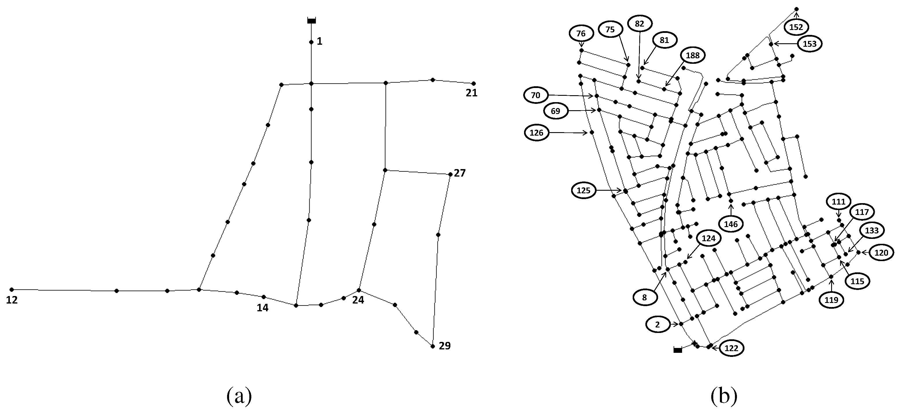
The proposed sensor placement approach presented in the previous sections is applied to two networks. The WDN of Hanoi in Vietnam [
34] is the first case study. This academic benchmark has been used in several works [
35,
36], where the objective was either to design the network or to optimize the operations performed within it. It consists of one reservoir, 31 demand nodes and 34 pipes, as shown in
Figure 1a. The second case study is based on the WDN of Limassol in Cyprus proposed as a test case in the EFFINET European project [
37]. This real network has already been used in leak location and sensor placement works [
21] and consists of one reservoir, 197 demand nodes and 239 pipes, as shown in
Figure 1b. All of the experiments were performed in MATLAB, using a Windows 7 computer with a Pentium Dual Core processor of 2 GHz, a memory (RAM) of 4 GB and a 64-bit operating system. The network models are simulated using the EPANET software [
24]. Leak magnitudes are simulated by changing a node emitter coefficient (
) that is related to the flow rate through the following equation:
where
q is the flow rate,
p is the fluid pressure and
γ is the pressure exponent. In the Hanoi network, in order to build the leak signatures, seven
values are considered going from two to eight with a step size of one, which leads to leak magnitudes varying from 20 to 80 liters per second (lps), which represent 1.7% of the total demand. For the Limassol network, seven
are also used going from
to
with a step size of
, which leads to leaks varying from 2 lps to 6 lps that represent 1% of the total demand.
In the following tables, the optimal sensor placements presented are the ones for which the number of overlaps between leak signature domains is minimum. Additionally, the efficiency is provided, which corresponds to the percentage of leaks correctly located. This performance index is computed by testing leaks in all possible nodes with all possible magnitudes within the range used to build the signature models and domains. The measurements are simulated with a random Gaussian white noise with the mean amplitude corresponding to of the expected measurement value.
Figure 1.
The Hanoi (a) and Limassol (b) water distribution networks (WDNs) used as benchmarks to evaluate the sensor placement method.
Figure 1.
The Hanoi (a) and Limassol (b) water distribution networks (WDNs) used as benchmarks to evaluate the sensor placement method.
5.1. Semi-Exhaustive Search Application
First, the semi-exhaustive approach is tested in the case of 2, 3 and 4 sensors for the Hanoi WDN. Results are summarized in
Table 1. It can be noticed that the method allows one to obtain an efficiency of
,
i.e., the percentage of correct leak locations, with two sensors and increases up to
in the case of four sensors. Notice also how the computational time tends to increase exponentially with the number of sensors implied, which comes from the fact that all possible sensor combinations have to be considered despite the lazy evaluation mechanism introduced.
Table 1.
Sensor placement in the Hanoi network using the semi-exhaustive approach.
Table 1.
Sensor placement in the Hanoi network using the semi-exhaustive approach.
| Sensors | Node Indexes | Overlaps | Efficiency (%) | Time (s) |
|---|
| 2 | 12, 21 | 5 | 93.1 | 11.2 |
| 3 | 12, 21, 29 | 1 | 98.6 | 181.0 |
| 4 | 1, 12, 21, 29 | 0 | 100.0 | 1637.5 |
In the Limassol network (see
Table 2), the semi-exhaustive search in the case of two sensors leads to evaluating
possible placements, which takes more than 5 h. The best configuration obtained gives a total of 253 overlaps and an efficiency of
. With three sensors, there are more than
possible placements, and it is not possible to test all of them in a reasonable time. Thus, we propose to start with the best result when placing two sensors and search for the best third sensor to add. This test will serve as a reference to evaluate the performance of the stochastic optimization approaches later on. The best third sensor is found in 541 s at Node 75, which leads to 166 overlaps and a final efficiency of
.
Table 2.
Sensor placement in the Limassol network using the semi-exhaustive approach.
Table 2.
Sensor placement in the Limassol network using the semi-exhaustive approach.
| Sensors | Node Indexes | Overlaps | Efficiency (%) | Time (s ) |
|---|
| 2 | 8, 152 | 253 | 60.6 | |
| 2 + 1 | 8, 75, 152 | 166 | 72.0 | + 0.54 |
These results show how the semi-exhaustive search allows a good leak detection efficiency thanks to the optimal sensor placement, but is clearly limited to small networks.
5.2. Application of GA and PSO Approaches
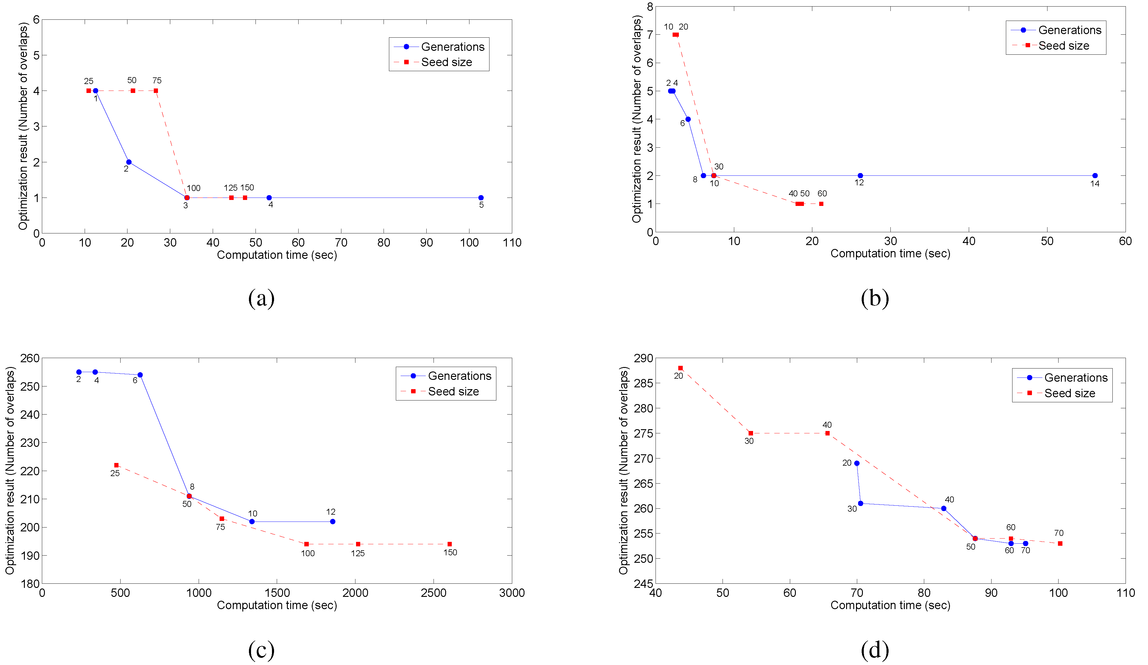
Before the application of the GA and PSO approaches, an analysis to determine the best parameter selection has been performed. In this analysis, the size of the seed matrix and the number of generations for each of the networks are chosen after several tests. The seed size is the number of rows in the initialization matrix used at the beginning of the search in the algorithm. This matrix is full of possible random solutions for the sensor placement. First, a seed size is selected to run the test in order to select the appropriate number of generations. Then, the tests are repeated varying the seed size and keeping the number of generations according to the previous result. The results of the tests are shown in
Figure 2.
Once the appropriate seed size and number of generations have been selected, several executions of the optimization process with different seed initializations are performed to improve the search efficiency. That is, whatever the method is, it is run several times (each run is called an iteration), and at each iteration, the best solution found is saved and included in the seed matrix of the next iteration. This is clearly a non-standard way to use GA/PSO, but such an approach was chosen during the implementation process after some trials, because it proved to be an efficient way to search for the global optimum. In comparison, a single GA/PSO iteration, but involving more generations, tends to be more easily trapped in local minima. On the opposite side, including more iterations (each with less generations) allows the approach to extend the search when profiting from the solutions from precedent iterations. As an example, when placing two sensors in the Limassol network, running 10 iterations with five generations in each of them gives as a result a placement with 253 overlaps, while running a single iteration with 50 generations finds as the best placement a result with 263 overlaps. As we can see, the iterations approach is more efficient than a single iteration with more generations.
In the case of the Hanoi network, the parameters after the tests are selected as follows: For the GA, the seed matrix was set to 100 rows filled with random solutions, and three generations are allowed. For the GA, three iterations were allowed in order to increase the efficiency of the method. For the PSO, a seed matrix of 50 rows is selected, and 10 generations are allowed. The PSO algorithm is run 50 times (i.e., 50 iterations were allowed) in order to increase the efficiency.
Figure 2.
Evaluation of the parameters to select for application of GA and PSO. (a) Tuning for the GA in the Hanoi network; (b) tuning for the PSO in the Hanoi network; (c) tuning for the GA in the Limassol network; (d) tuning for the PSO in the Limassol network.
Figure 2.
Evaluation of the parameters to select for application of GA and PSO. (a) Tuning for the GA in the Hanoi network; (b) tuning for the PSO in the Hanoi network; (c) tuning for the GA in the Limassol network; (d) tuning for the PSO in the Limassol network.
For the Limassol network, the parameters were selected as follows: A seed matrix of 100 rows and five generations are allowed. The GA algorithm is run 10 times (i.e., a total of 10 iterations). For the PSO, a seed matrix of 50 rows was selected allowing 50 generations. The PSO algorithm will be run 150 times; this means that we are allowing 150 iterations.
5.2.1. Tests on the Hanoi WDN
Both GA and PSO approaches are applied to the Hanoi example. In the following, we show the results obtained after several tests performed with both methods. It is important to mention that all of the conclusions correspond to the cases observed with the settings chosen for both the GA and PSO methods. Results obtained when only a single time instant was considered are shown in
Table 3. As one can see, both methods find optimal solutions in all cases, since, in this case, the number of overlaps matches the results of the semi-exhaustive approach. However, note that sometimes, the solution corresponds to a different sensor combination, but resulting in an equivalent efficiency. It is remarkable that GA and PSO find the optimum in a much faster way than with the semi-exhaustive approach when the number of sensors starts to increase. Finally, PSO tends to be substantially faster on these scenarios.
Table 3.
Sensor placement in the Hanoi WDN using stochastic approaches and a single time instant.
Table 3.
Sensor placement in the Hanoi WDN using stochastic approaches and a single time instant.
| Sensors | Node Indexes | Overlaps | Efficiency (%) | Time (s) |
|---|
| GA | PSO | GA | PSO | GA | PSO | GA | PSO |
|---|
| 2 | 12, 21 | 12, 21 | 5 | 5 | 93.1 | 93.1 | 69.9 | 17.3 |
| 3 | 12, 21, 27 | 12, 14, 21 | 1 | 1 | 98.6 | 98.6 | 113.9 | 38.0 |
| 4 | 1, 12, 21, 29 | 1, 12, 21, 24 | 0 | 0 | 100.0 | 100.0 | 119.9 | 57.5 |
GA and PSO approaches were also applied to the Hanoi example when considering a 24-h time horizon to build the LSS model. Results are shown in
Table 4, where it can be seen that the efficiency tends to increase compared to the tests based on a single time instant, but only slightly and at the expense of an important increase in computational cost.
Table 4.
Sensor placement in the Hanoi WDN using stochastic approaches and a time horizon analysis.
Table 4.
Sensor placement in the Hanoi WDN using stochastic approaches and a time horizon analysis.
| Sensors | Node Indexes | Overlaps | Efficiency (%) | Time (s ) |
|---|
| GA | PSO | GA | PSO | GA | PSO | GA | PSO |
|---|
| 2 | 12, 21 | 12, 21 | 7 | 7 | 93.5 | 93.5 | | 0.5 |
| 3 | 12, 14, 21 | 12, 14, 21 | 1.08 | 1.08 | 98.8 | 98.8 | | |
| 4 | 1, 12, 21, 27 | 1, 12, 21, 27 | 0.08 | 0.08 | 100.0 | 100.0 | | |
5.2.2. Tests on the Limassol WDN
GA and PSO approaches were also applied to the more complex case of the Limassol network. The results obtained considering only a single time instant are shown in
Table 5.
First, one can see that with two sensors, both GA and PSO find the optimum solution already found with the semi-exhaustive method. Moreover, in the case of three sensors, solutions found by means of these two methods are better than in the case of the
semi-exhaustive approach presented in the previous subsection and with a lower computational cost. Besides, it should be remarked that with the considered settings, PSO works more quickly than GA, but when the problem increases,
i.e., when more sensors are installed and more combinations are possible, GA finds better combinations. From additional experiments not reported in the table, we have seen that even by increasing the number of iterations, the PSO tends to be trapped in a local suboptimum. Such behavior has already been reported in the literature [
38]. It may be explained by the fact that PSO has the memory of past successes and tends to explore around the recorded configurations, whereas when it is necessary to leap from one region to another distant region, crossover operations like those in GA are probably preferred [
39]. Besides, it should be remarked that with the considered settings, PSO works more quickly than GA, but when the problem increases,
i.e., when more sensors are installed and more combinations are possible, GA finds better combinations. From additional experiments not reported in the table, we have seen that even by increasing the number of iterations, the PSO tends to be trapped in a local suboptimum. Such behavior has already been reported in the literature [
38]. This may be explained by the fact that PSO has the memory of past successes and tends to explore around the recorded configurations, whereas when it is necessary to leap from one region to another distant region, crossover operations, like those in GA, are probably preferred [
39].
Table 5.
Sensor placement in the Limassol WDN using stochastic approaches and a single time instant.
Table 5.
Sensor placement in the Limassol WDN using stochastic approaches and a single time instant.
| Sensors | Node Indexes | Overlaps | Efficiency (%) | Time (s ) |
|---|
| GA | PSO | GA | PSO | GA | PSO | GA | PSO |
|---|
| 2 | 8, 152 | 8, 152 | 253 | 253 | 60.6 | 60.6 | | |
| 3 | 75, 120, 152 | 76, 115, 152 | 145 | 151 | 74.1 | 74.0 | | |
| 4 | 76, 82, 120, 152 | 69, 82, 119, 152 | 114 | 131 | 78.0 | 76.2 | | |
| 5 | 75, 82, 120, 126, 152 | 70, 115, 125, 152, 188 | 106 | 122 | 79.0 | 77.4 | | |
GA and PSO were also applied to the Limassol network while incorporating a time horizon analysis. However, only the case of two and three sensors was considered, since the computational time becomes prohibitive for a higher number of sensors. Moreover, for the GA method, only one iteration
is authorized and 15 iterations for the PSO instead of the 10 and 150 iterations used respectively for the single time instant case. Results are summarized in
Table 6. It shows that contrary to the Hanoi case, for this more complex scenario, the incorporation of a time horizon significantly improves the efficiency. It is remarkable to see that the LSS-based leak location method relying on only three sensors and the GA method is able to locate almost
of the leaks correctly. However, the time horizon analysis clearly comes at the expense of an important additional computational cost.
Table 6.
Sensor placement in the Limassol WDN using stochastic approaches and a time horizon analysis.
Table 6.
Sensor placement in the Limassol WDN using stochastic approaches and a time horizon analysis.
| Sensors | Node Indexes | Overlaps | Efficiency (%) | Time (s ) |
|---|
| GA | PSO | GA | PSO | GA | PSO | GA | PSO |
|---|
| 2 | 124, 153 | 124, 153 | 424.8 | 424.8 | 77.7 | 77.7 | 32.3 | 27.5 |
| 3 | 76, 133, 169 | 75, 122, 117 | 289.8 | 306.2 | 84.9 | 84.8 | | |
5.3. Optimization Criterion and Leak Detection Efficiency
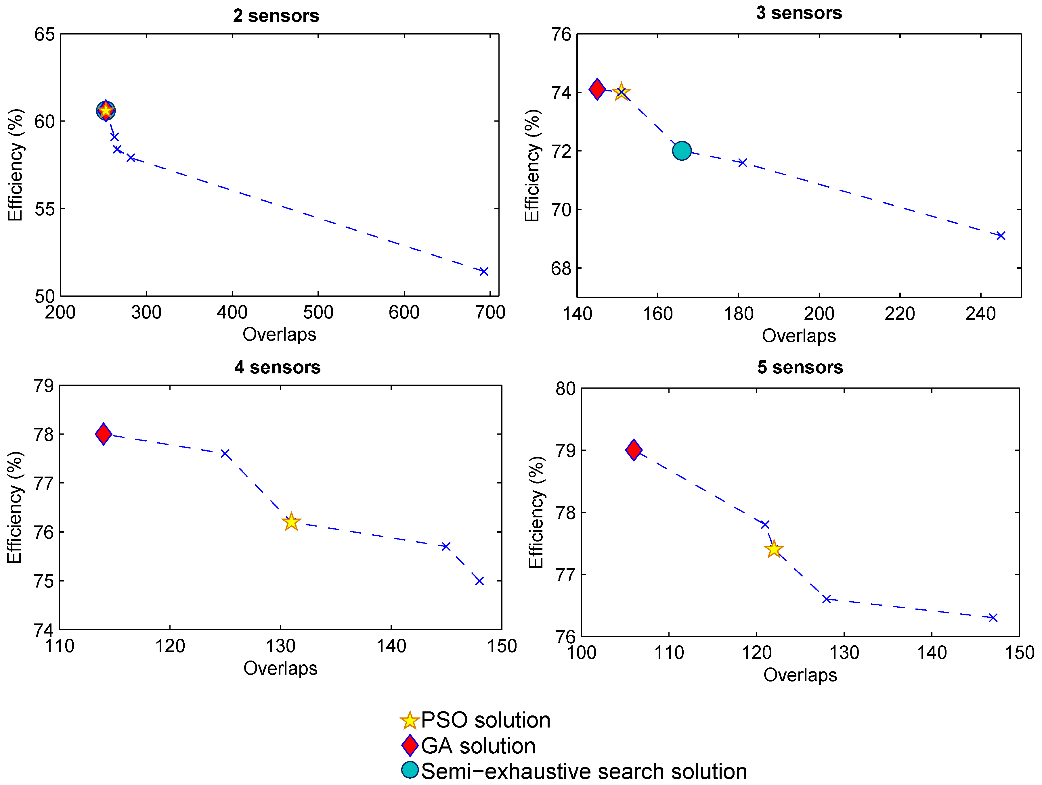
Whatever the optimization resolution method used, the optimization problem presented above relies on the minimization of intersections between leak signature domains. However, it is important to verify that decreasing the number of intersections effectively improves the leak location efficiency. To be relevant, comparisons must be made on scenarios involving the same number of sensors to place, since otherwise, the number of overlapping domains to be checked would be different.
Figure 3 presents for different number of sensors placed in the Limassol network, the variation of leak location efficiency as a function of the number of overlaps found. These values are taken directly from the results of the optimization methods or by manually choosing combinations of nodes already appearing within the set of solutions of these methods. This figure clearly illustrates the negative correlation between the efficiency and the number of overlaps found. It is important to highlight how the performance of the correct sensor placement clearly improves the efficiency of the leak location method. In this graph, we can see that a higher efficiency can be reached with four sensors when they are optimally placed, whereas such efficiency will not be achieved using five sensors if they are not optimally installed. Thanks to this analysis, the importance of optimizing the sensor placement according to the leak location method to be used is proven.
Figure 3.
Efficiency in leak location according to the number of overlaps in the configuration for the Limassol network.
Figure 3.
Efficiency in leak location according to the number of overlaps in the configuration for the Limassol network.
6. Conclusions
This paper describes a new approach to place a given set of sensors in a WDN in order to maximize the efficiency of the leak detection. The solution is motivated by the application of an original leak representation method based on what is known as the leak signature space. A semi-exhaustive method based on a lazy evaluation mechanism is proposed to solve low complexity problems. For more complex scenarios, either a GA or a PSO method is applied to the underlying optimization problem. Results demonstrate the validity of the approach. They also show that with the parameters selected for the stochastic optimization methods, PSO tends to give results faster than the GA approach and is very effective for small networks or few sensors. However, the solutions found by the GA tend to correspond to better placements and with higher efficiency for larger networks or more sensors. It also appears that a time horizon analysis can significantly improve the performance in the case of complex scenarios. Finally, the negative correlation between the optimization function and the efficiency of the leak detection method is verified.
As future work, we would like to extend this work to more complex WDN, such as the Barcelona network used in [
11], consisting of 3320 nodes. Furthermore, the location of smaller leaks would be interesting to address, taking into account that they can be easily masked by the noise in the sensors. Finally, we have seen that even with the stochastic optimization tools proposed in this paper, the application of the time horizon analysis was not tractable for the Limassol network with more than three sensors. Then, we would like to investigate the possible application of a parallel computation in a multi-core processor, combined with the possibility of an accurate tuning method for the selection of the parameters used in the GA and PSO approaches. Furthermore, we would like to investigate new approaches to tackle this limitation and obtain an improved leak location efficiency.


