
Performance Assessment of Hydrological Models Considering Acceptable Forecast Error Threshold

Abstract
:1. Introduction
- (1)
- What is the correlation between the rainfall forecast error and peak flood forecast error, is it statistically significant?
- (2)
- How to calculate the reliability index of a hydrological model based on the reliability theory, under the context of correlated forecast errors considering two scenarios, single failure mode and double failure mode (see Section 4)?
- (3)
- What is the effect of different types of the performance function on the reliability index of a hydrological model?
- (4)
- What is the change law for the reliability index of a hydrological model with regard to the variable correlation between the two forecast errors?
2. Material and Methods
2.1. Simple Introduction to Reliability Theory
2.2. FOSM Method
2.3. Ditlevsen’s Bounds Method
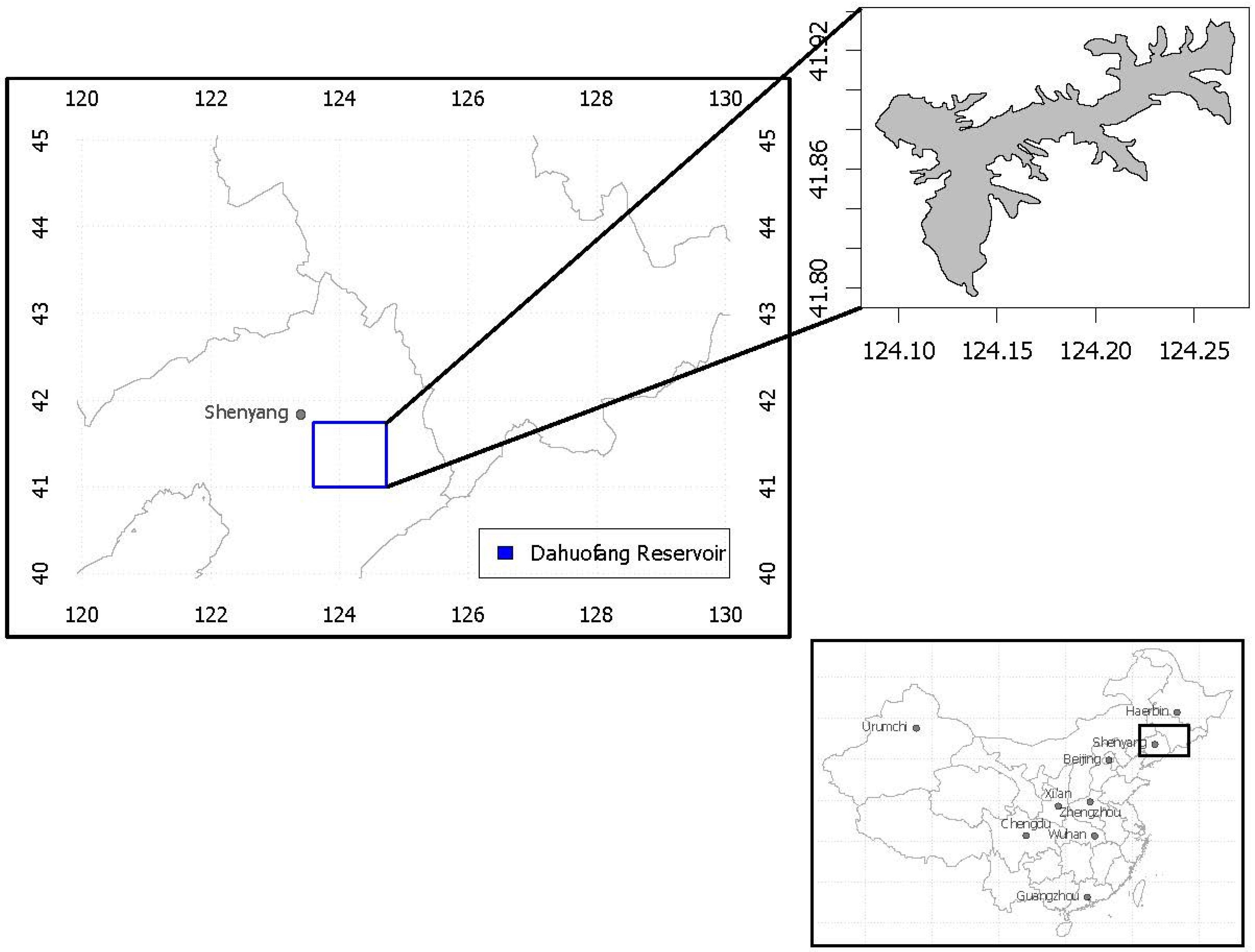
3. Study Area


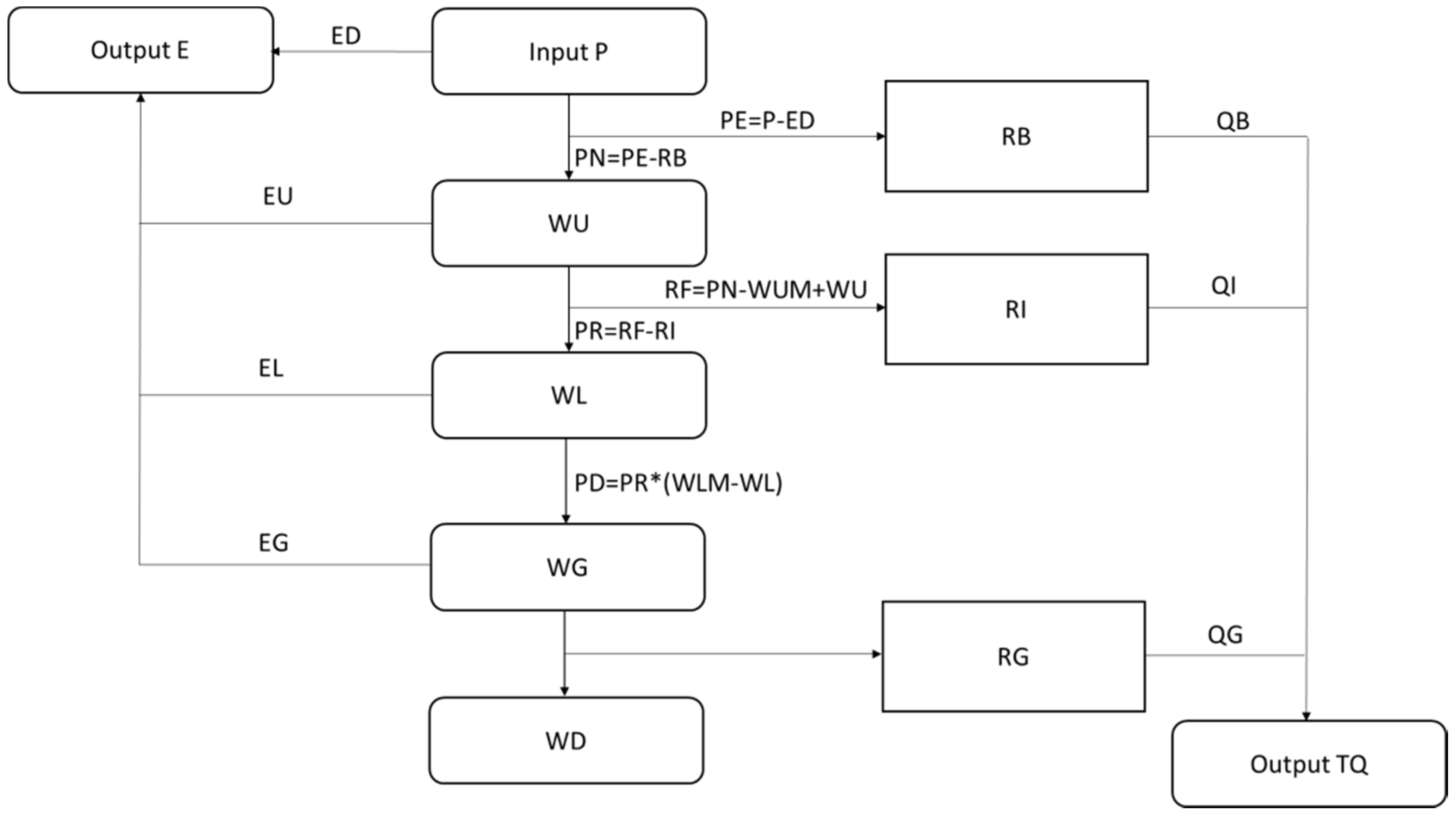
| Parameters | Description | Parameters | Description |
|---|---|---|---|
| P | precipitation | RB | surface runoff |
| ED | pan evaporation | RI | Interflow runoff |
| PE | effective precipitation | RG | groundwater runoff |
| PN | infiltrative precipitation | RF | infiltration |
| WU | surface upper layer water storage | PR | infiltration after detaining interflow runoff |
| WUM | storage capacity of upper layer | WG | groundwater storage |
| WL | surface lower layer water storage | WD | deep groundwater storage |
| WLM | storage capacity of lower layer | PD | lower infiltration |
| EU | upper layer evaporation | EL | lower layer evaporation |
| EG | groundwater evaporation | QB | surface streamflow |
| QI | interflow streamflow | QG | groundwater streamflow |
| Year | Number of Floods |
|---|---|
| 1964 | 5 |
| 1985 | 4 |
| 1995 | 3 |
| 1996 | 3 |
| Items | Qualified Rate (%) | Correlation of Forecast Errors | ||
|---|---|---|---|---|
| Pearson | Kendall | Spearman | ||
| Rainfall forecast | 93.55 | 0.40 * | 0.50 ** | 0.68 ** |
| Flood forecast | 80.65 | |||


4. Results and Discussion
4.1. Single Failure Mode
4.2. Double Failure Mode
4.2.1. Unknown Performance Function
| Structure Types | Correlation Coefficient | Wide Bounds Method | Narrow Bounds Method |
|---|---|---|---|
| Serial | 0.40 | [0.17, 0.24] | [0.22, 0.22] |
| Parallel | [0.015, 0.085] | [0.017, 0.035] |
4.2.2. Known Performance Function

4.3. Discussion
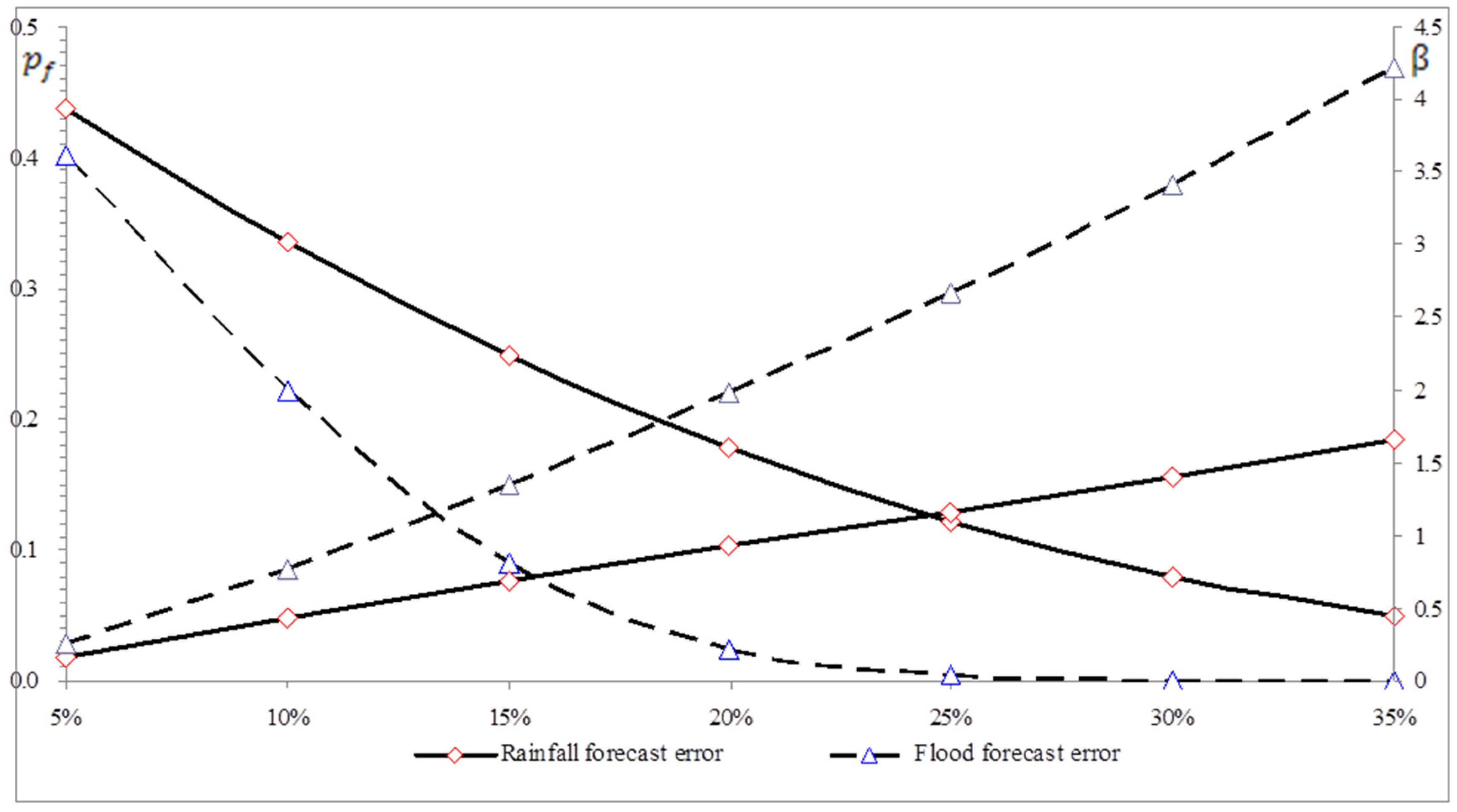
4.3.1. The Acceptable Threshold Value of the Performance Function
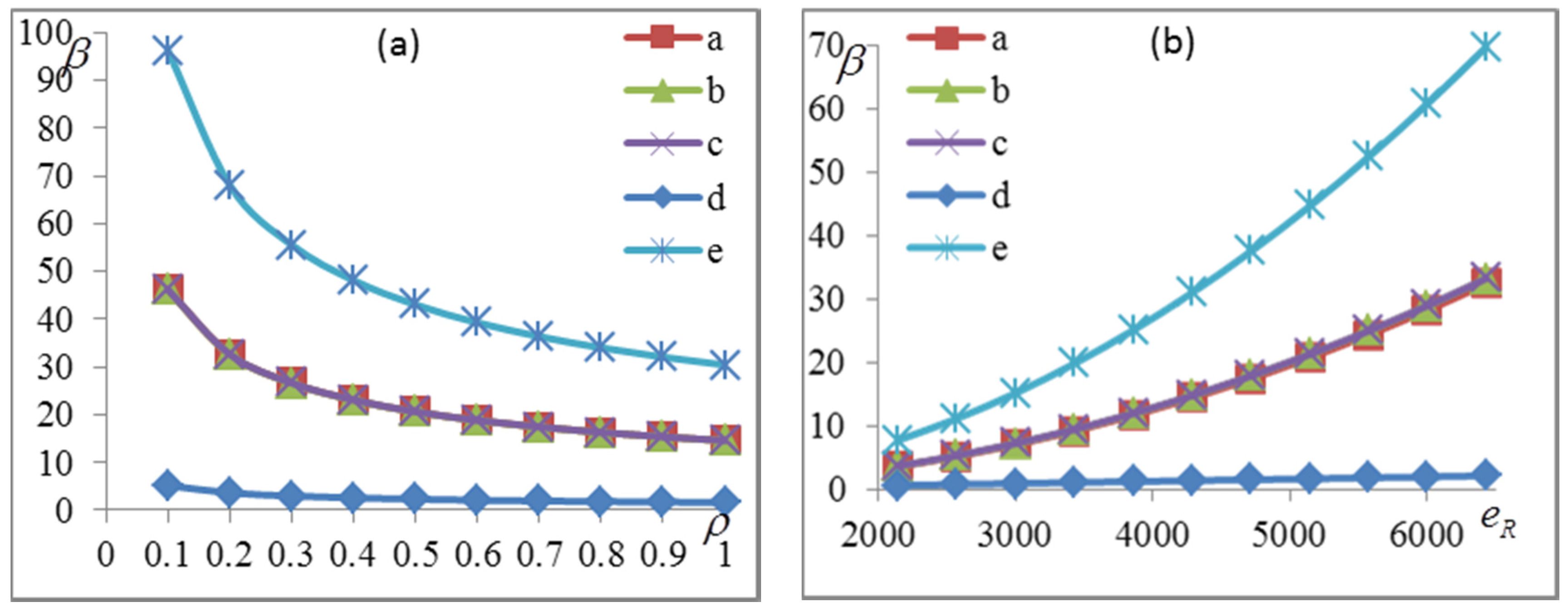
4.3.2. Correlation between the Basic Variables of the Performance Function
5. Conclusions
- (1)
- The sensitivity of performance function on different acceptable threshold of forecast error are different, and the variation of the flood forecast error seems to change nonlinearly with their acceptable threshold and the rainfall forecast error changes almost linearly with their acceptable threshold.
- (2)
- The correlation between the rainfall forecast error and the flood forecast has great impact on the evaluation of performance of hydrological model, and the reliability index of the hydrological model system decreases when the correlation increases positively. The resistance has great impact on the evaluation of performance of a hydrological model, which means that larger resistance indicates higher reliability index.
Acknowledgments
Author Contributions
Conflicts of Interest
References
- Nash, J.E.; Sutcliffe, J.V. River flow forecasting through conceptual models—Part I: A discussion of principles. J. Hydrol. 1970, 10, 282–290. [Google Scholar] [CrossRef]
- Willems, P. Parsimonious rainfall–runoff model construction supported by time series processing and validation of hydrological extremes—Part 2: Intercomparison of models and calibration approaches. J. Hydrol. 2014, 510, 591–609. [Google Scholar] [CrossRef]
- Van Werkhoven, K.; Wagener, T.; Reed, P.; Tang, Y. Sensitivity-guided reduction of parametric dimensionality for multi-objective calibration of watershed models. Adv. Water Resour. 2009, 32, 1154–1169. [Google Scholar] [CrossRef]
- Vrugt, J.A.; Diks, C.G.H.; Gupta, H.V.; Bouten, W.; Verstraten, J.M. Improved treatment of uncertainty in hydrologic modelling: Combining the strengths of global optimization and data assimilation. Water Resour. Res. 2005, 41. [Google Scholar] [CrossRef]
- Neumann, M.B.; Gujer, W. Underestimation of uncertainty in statistical regression of environmental models: Influence of model structure uncertainty. Environ. Sci. Technol. 2008, 42, 4037–4043. [Google Scholar] [CrossRef] [PubMed]
- Willems, P. A time series tool to support the multi-criteria performance evaluation of rainfall–runoff models. Environ. Model. Softw. 2009, 24, 311–321. [Google Scholar] [CrossRef]
- Sorooshian, S.; Dracup, J. Stochastic parameter estimation procedures for hydrologic rainfall–runoff models: Correlated and heteroscedastic error cases. Water Resour. Res. 1980, 29, 1185–1194. [Google Scholar] [CrossRef]
- Sorooshian, S. Parameter estimation of rainfall–runoff models with heteroscedastic streamflow errors—The noninformative data case. J. Hydrol. 1981, 52, 127–138. [Google Scholar] [CrossRef]
- Kelly, K.S.; Krzysztofowicz, R. A bivariate meta-Gaussian density for use in hydrology. Stoch. Hydrol. Hydraul. 1997, 11, 17–31. [Google Scholar] [CrossRef]
- Xu, C.Y. Statistical analysis of a conceptual water balance model, methodology and case study. Water Resour. Manag. 2001, 15, 75–92. [Google Scholar] [CrossRef]
- Montanari, A.; Brath, A. A stochastic approach for assessing the uncertainty of rainfall–runoff simulations. Water Resour. Res. 2004, 40. [Google Scholar] [CrossRef]
- Mantovan, P.; Todini, E. Hydrological forecasting uncertainty assessment: Incoherence of the GLUE methodology. J. Hydrol. 2006, 330, 368–381. [Google Scholar] [CrossRef]
- Kavetski, D.; Fenicia, F.; Clark, M.P. Impact of temporal data resolution on parameter inference and model identification in conceptual hydrological modelling: Insights from an experimental catchment. Water Resour. Res. 2011, 47. [Google Scholar] [CrossRef]
- Evin, G.; Thyer, M.; Kavetski, D.; McInerney, D.; Kuczera, G. Comparison of joint versus postprocessor approaches for hydrological uncertainty estimation accounting for error autocorrelation and heteroscedasticity. Water Resour. Res. 2014, 50, 2350–2375. [Google Scholar] [CrossRef]
- Krzysztofowicz, R. Integrator of uncertainties for probabilistic river stage forecasting: Precipitation-dependent model. J. Hydrol. 2001, 249, 69–85. [Google Scholar] [CrossRef]
- Hostache, R.; Matgen, P.; Montanari, A.; Montanari, M.; Hoffmann, L.; Pfister, L. Propagation of uncertainties in coupled hydro-meteorological forecasting systems: A stochastic approach for the assessment of the total predictive uncertainty. Atmos. Res. 2011, 100, 263–274. [Google Scholar] [CrossRef]
- Nester, T.; Komma, J.; Viglione, A.; Blöschl, G. Flood forecast errors and ensemble spread—A case study. Water Resour. Res. 2012, 48. [Google Scholar] [CrossRef]
- Yazdi, J.; Salehi-Neyshabouri, S.A.A.; Golian, S. A stochastic framework to assess the performance of flood warning systems based on rainfall–runoff modeling. Hydrol. Process. 2014, 28, 4718–4731. [Google Scholar] [CrossRef]
- Dogulu, N.; López, P.; Solomatine, D.P.; Weerts, A.H.; Shrestha, D.L. Estimation of predictive hydrologic uncertainty using the quantile regression and UNEEC methods and their comparison on contrasting catchments. Hydrol. Earth Syst. Sci. 2015, 19, 3181–3201. [Google Scholar] [CrossRef]
- Han, S.W.; Wen, Y.K. Method of reliability-based seismic design. 1: Equivalent nonlinear systems. J. Struct. Eng. ASCE 1997, 123, 256–263. [Google Scholar] [CrossRef]
- Wen, Y.K. Reliability and performance-based design. Struct. Saf. 2001, 23, 407–428. [Google Scholar] [CrossRef]
- Mohammadzadeh, S.; Ahadi, S.; Nouri, M. Stress-based fatigue reliability analysis of the rail fastening spring clip under traffic loads. Laitin Am. J. Solids Struct. 2014, 11, 993–1011. [Google Scholar] [CrossRef]
- Rakoczy, A.M.; Nowak, A.S. Resistance factors for lightweight concrete members. ACI Struct. J. 2014, 111, 103–111. [Google Scholar]
- Silva, J.E.; Garbatov, Y.; Soares, G.C. Reliability assessment of a steel plate subjected to distributed and localized corrosion wastage. Eng. Struct. 2014, 59, 13–20. [Google Scholar] [CrossRef]
- Loucks, D.P.; Stedinger, J.R.; Haith, D.A. Water Resources System Planning and Analysis; Prentice-Hall: Upper Saddle River, NJ, USA, 1988. [Google Scholar]
- Ganji, A.; Jowkarshorijeh, L. Advance first order second moment (AFOSM) method for single reservoir operation reliability analysis: A case study. Stoch. Environ. Res. Risk Assess. 2012, 26, 33–42. [Google Scholar] [CrossRef]
- Augusti, G.; Baratta, A.; Casciati, F. Probabilistic Methods in Structural Engineering; Chapman and Hall: London, UK, 1984. [Google Scholar]
- Rubinstein, R.Y.; Kroese, D.P. Simulation and Monte-Carlo Method; Wiley: New York, NY, USA, 2007. [Google Scholar]
- Hasofer, A.M.; Lind, N.C. Exact and invariant second-moment code format. J. Eng. Mech. Div. AMSE 1974, 100, 111–121. [Google Scholar]
- Rackwitz, R.; Fiessler, B. Structural reliability under combined random load sequences. Comput. Struct. 1978, 9, 489–494. [Google Scholar] [CrossRef]
- Xu, L.; Cheng, G.D. Discussion on: Moment methods for structural reliability. Struct. Saf. 2003, 25, 192–199. [Google Scholar] [CrossRef]
- Faravelli, L. Response surface approach for reliability analysis. J. Struct. Mech. ASCE 1989, 115, 2763–2781. [Google Scholar] [CrossRef]
- Maskey, S.; Guinot, V. Improved first-order second moment method for uncertainty estimation in flood forecasting. Hydrol. Sci. J. 2003, 48, 183–196. [Google Scholar] [CrossRef]
- Shinozuka, M. Basic analysis of structural safety. J. Struct. Div. ASCE 1983, 109, 721–740. [Google Scholar] [CrossRef]
- Rosenblatt, M. Remark on a multivariate transformation. Ann. Math. Stat. 1952, 23, 470–472. [Google Scholar] [CrossRef]
- Liu, P.L.; der Kiureghian, A. Multivariate distribution models with prescribed marginal and covariances. Probab. Eng. Mech. 1986, 1, 105–112. [Google Scholar] [CrossRef]
- Schoutens, W. Stochastic Processes and Orthogonal Polynomial; Springer-Verlag: New York, NY, USA, 2000. [Google Scholar]
- Ditlevsen, O. Narrow reliability bounds for structural systems. J. Struct. Mech. 1979, 7, 453–472. [Google Scholar] [CrossRef]
- Cornell, C.A. Bounds on the reliability of structural systems. J. Struct. Div. ASCE 1967, 93, 171–200. [Google Scholar]
- Kounias, E.G. Bounds for the probability of a union with applications. Ann. Math. Stat. 1968, 39, 2154–2158. [Google Scholar] [CrossRef]
- Horton, R.E. The role of infiltration in the hydrologic cycle. Trans. Am. Geophys. Union 1933, 14, 446–460. [Google Scholar] [CrossRef]
- Zhai, S.Y. Risk Analysis of Flood Forecasting and Flood Regulation under Different Limited Level. Master’s Thesis, Nanjing Hydraulic Research Institute, Nanjing, China, 2010. [Google Scholar]
- Lilliefors, H. On the Kolmogorov-Smirnov test for normality with mean and variance unknown. J. Am. Stat. Assoc. 1967, 62, 399–402. [Google Scholar] [CrossRef]
- Lilliefors, H. On the Kolmogorov-Smirnov test for the exponential distribution with mean unknown. J. Am. Stat. Assoc. 1969, 64, 387–389. [Google Scholar] [CrossRef]
- General Administration of Quality Supervision, Inspection and Quarantine of P.R.C. (GAQSIQC). Standard for Hydrological Information and Hydrological Forecasting; (GB/T 22482-2008); China Water & Power Press: Beijing, China, 2008.
- Hohenbichler, M.; Rackwitz, R. First-order concepts in system reliability. Struct. Saf. 1983, 1, 177–188. [Google Scholar] [CrossRef]
- Kamruzzaman, M.; Shahriar, M.S.; Beecham, S. Assessment of Short Term Rainfall and Stream Flows in South Australia. Water 2014, 6, 3528–3544. [Google Scholar] [CrossRef]
- Callegari, M.; Mazzoli, P.; de Gregorio, L.; Notarnicola, C.; Pasolli, L.; Petitta, M.; Pistocchi, A. Seasonal River Discharge Forecasting Using Support Vector Regression: A Case Study in the Italian Alps. Water 2015, 7, 2494–2515. [Google Scholar] [CrossRef] [Green Version]
© 2015 by the authors; licensee MDPI, Basel, Switzerland. This article is an open access article distributed under the terms and conditions of the Creative Commons Attribution license (http://creativecommons.org/licenses/by/4.0/).
Share and Cite
Dong, Q.; Lu, F. Performance Assessment of Hydrological Models Considering Acceptable Forecast Error Threshold. Water 2015, 7, 6173-6189. https://doi.org/10.3390/w7116173
Dong Q, Lu F. Performance Assessment of Hydrological Models Considering Acceptable Forecast Error Threshold. Water. 2015; 7(11):6173-6189. https://doi.org/10.3390/w7116173
Chicago/Turabian StyleDong, Qianjin, and Fan Lu. 2015. "Performance Assessment of Hydrological Models Considering Acceptable Forecast Error Threshold" Water 7, no. 11: 6173-6189. https://doi.org/10.3390/w7116173