1. Introduction
Typically, water quality samples are costly to collect and to analyze. Water quality samples are collected by various sampling frequencies [
1] and thus may not be collected over the period of streamflow data and further are not typically collected at the same data frequency (or interval) as streamflow data. Few water quality datasets have been collected by frequent water quality sampling (
i.e., short sampling intervals) such as on an hourly basis [
2]; however, water quality data have often been collected infrequently compared to streamflow data frequencies [
3,
4].
Thus, water quality data are often estimated using statistical methods such as regression models from measurements made intermittently in a certain period of time [
5]. Regression models are used extensively to interpolate intermittent water quality data and are often simple linear forms using logarithmic transformations [
6,
7]. Various water quality data sampling frequencies have been used to estimate pollutant loads with regression models and to explore what sampling frequencies are appropriate for regression model uses [
5,
8,
9,
10,
11]. Acceptable load estimates were provided by regression models with water quality data collected biweekly or monthly supplemented with storm samples [
5,
8,
9], while in other cases, regression models often provided poor load estimates (
i.e., load estimates with large error) when the number of water quality data were small [
8] or when water quality datasets did not follow a normal distribution [
10]. Moreover, regression models displayed differences of up to 65% in annual nitrate-N load estimates [
11].
In addition to sampling frequencies and regression models, water quality parameters are also influential to load estimation, since each water quality parameter has different behaviors in watersheds. Streamflow and total nitrogen concentration displayed poor relationships, and sediment concentration and streamflow showed significant correlation in pasture watersheds [
12]. In another study, baseflow was a major source of nitrate loads to streamflow since nitrate concentration and baseflow displayed a proportional relationship; however, orthophosphate concentration was not related to baseflow behavior [
13].
LOAD ESTimator (LOADEST) [
14] is used to estimate pollutant loads using streamflow data, water quality concentration data, and regression model coefficients using one of 11 regression models. LOADEST has been used to estimate daily pollutant loads for various water quality parameters with various sample sizes (or sampling frequencies) including weekly [
15], monthly [
16], or bimonthly [
17,
18] collected water quality samples. The Load Interpolation Tool (LOADIN) [
19] is a web-based tool to estimate pollutant loads from streamflow and intermittent water quality data. LOADIN has the same purpose as LOADEST and requires streamflow and water quality data to estimate pollutant loads. However, LOADIN uses a different regression model and different approach to calibrate the model coefficients.
In this study, the predictive ability of LOADEST and LOADIN was evaluated with six sampling frequencies for three water quality parameters, and appropriate regression models and water quality sampling frequencies were suggested to obtain accurate annual pollutant load estimates.
2. Materials and Methods
2.1. Water Quality Data Collection and Subsampling
Daily streamflow and water quality data were required to compute an observed “true load” and to create subsampled water quality datasets for LOADEST and LOADIN runs. Therefore, daily streamflow and water quality data for nitrogen, phosphorus, and sediment were collected from the National Center for Water Quality Research of Heidelberg University [
20] and the USGS Water-Quality Data for the Nation [
21] (
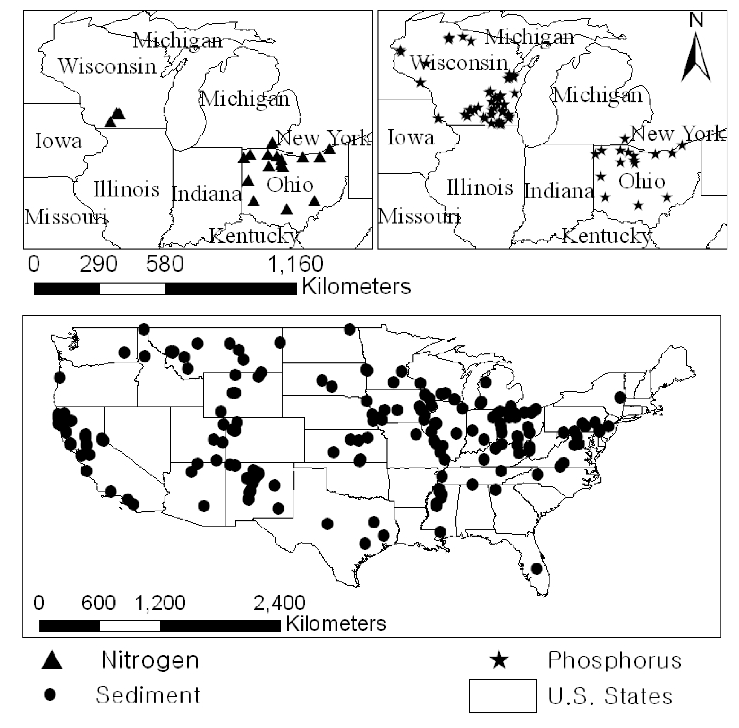
Figure 1). Daily nitrogen (Total Nitrogen; USGS Water Quality Parameter Code: 91058) data were collected from 21 stations, daily phosphorus (Phosphorus; USGS Water Quality Parameter Code: 91050) data were collected from 69 stations, and daily sediment (Suspended Sediment Discharge; USGS Water Quality Parameter Code: 80155) data were collected from 211 stations (
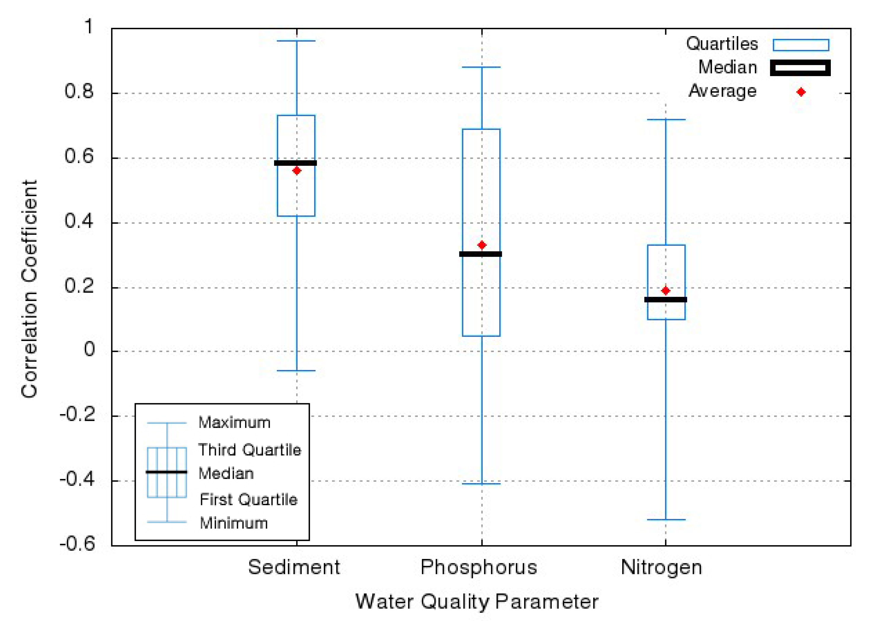
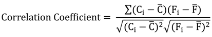
Table 1). The water quality data collected in the study displayed different relationships with streamflow. Correlation coefficients (Equation (1)) were computed to provide the relationships between streamflow and concentration data (
Figure 2). The averages of correlation coefficients were 0.6 for sediment concentration data, 0.3 for phosphorus concentration data, and 0.2 for nitrogen concentration data. Thus, sediment concentration data were most-closely correlated to streamflow, compared to phosphorus and nitrogen concentration data.
where Ci is concentration at time step i; C is mean of concentration data; Fi is streamflow at time step I; F and is mean of streamflow data.
Figure 1.
Locations of Daily Water Quality Data Stations.
Figure 1.
Locations of Daily Water Quality Data Stations.
Table 1.
Number of stations and daily water quality data values.
Table 1.
Number of stations and daily water quality data values.
| Water Quality Parameters | 1~10 years | 11~20 years | 21~37 years | Total |
|---|
| Nitrogen | 11 a
10,220 b | 5 a
28,835 b | 5 a
58,035 b | 21 a
97,090 b |
| Phosphorus | 59 a
56,940 b | 5 a
28,835 b | 5 a
58,035 b | 69 a
143,810 b |
| Sediment | 201 a
423,035 b | 5 a
28,835 b | 5 a
58,035 b | 211 a
509,905 b |
Figure 2.
Correlation Coefficients for Concentrations of Water Quality Parameters with Streamflow (adapted from Park, 2014 [
22]).
Figure 2.
Correlation Coefficients for Concentrations of Water Quality Parameters with Streamflow (adapted from Park, 2014 [
22]).
Six sampling frequencies were established with combinations of fixed intervals and inclusion of storm samples. The first three sampling frequencies represented collecting one water quality sample every week (weekly fixed interval sampling frequency), every two weeks (biweekly fixed interval sampling frequency), and every month (monthly fixed interval sampling frequency).
For fixed interval sampling, water quality data were selected on the same day every week, two weeks, and month so that weekly, biweekly, and monthly sampling had seven, fourteen, and twenty eight variants, respectively. For instance, the first subsampled water quality datasets for the weekly interval frequency were comprised of the water quality data observed on every Monday, while the second subsampled water quality datasets for the weekly interval frequency were comprised of the water quality data observed on every Tuesday. Therefore, seven subsampled water quality datasets were prepared for the weekly interval frequency. The first subsampled water quality datasets for the biweekly interval frequency were comprised of the water quality data observed on every alternate Monday, and the second subsampled water quality datasets for the biweekly interval frequency were comprised of water quality data observed on every alternate Tuesday. Therefore, fourteen subsampled water quality datasets were prepared for the biweekly interval frequency. The subsampling method for monthly interval frequencies was based on date. For instance, the first subsampled water quality dataset for monthly interval frequencies was comprised of the water quality data observed on the 1st day of each month, and the second subsampled water quality dataset for monthly interval frequencies was comprised of the water quality data observed on the 2nd day of each month.
The other three sampling frequencies termed “mixed interval sampling” included additional samples from within storm events while maintaining the same sampling intervals as the first three frequencies. Storm samples in the study were defined as water quality data collected from peak flows in the “high flow” regime that represent the upper 10 percent of flows for a given analysis period [
23].
2.2. Regression Models
The regression model coefficients in LOADEST are calibrated by three statistical methods which are Adjusted Maximum Likelihood Estimation (AMLE), Maximum Likelihood Estimation (MLE), and Least Absolute Deviation (LAD) [
14]. The AMLE and MLE methods assume that the calibration model error (or residuals) follows a normal distribution, and allow use of water quality datasets containing censored data [
24]. The LAD method is based on the assumption that the errors are independently and identically distributed random variables [
25].
LOADEST has 11 regression models, and one of them is selected manually or automatically (model number option 0). The first nine regression models numbered from 1 to 9 (Equations (2)–(10), left-hand side is logarithm pollutant load) are selectable by the automatic regression model selection, but the other regression models numbered 10 and 11 (Equations (11) and (12)) are used to estimate pollutant loads for specific periods defined by users. Therefore, LOADEST was executed ten times for each subsampled water quality dataset with model number 0 to investigate performance for automatic model selection of LOADEST and with model numbers 1 to 9 to evaluate each regression model for manual model selection. Subsampled water quality datasets were used for LOADEST and LOADIN runs.
where,
a0~6 are coefficients;
Q is streamflow;
dtime is decimal time; and
per is the period defined by the user [
14].
LOADIN employs a regression model comprised of streamflow, decimal time, and eight model coefficients (Equation (13)). LOADIN finds values of the eight model coefficients that minimize differences between modeled and observed loads using a genetic algorithm and given water quality datasets.
where, Li is pollutant load at time step i; Qi is streamflow at time step i.
The regression models in LOADEST assume that instantaneous load is an exponential function of data variables (e.g., streamflow) [
14]; however, the regression model in LOADIN assumes that instantaneous load is comprised of the pollutant load by flow and the pollutant load varying by time.
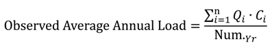
Annual pollutant loads estimated by the regression models in LOADEST and LOADIN were compared to annual loads calculated by multiplying daily streamflow by concentration measurements (Equation (14)).
where, i is day; Qi is streamflow on day i; Ci is concentration on day i; and Num.Yr is the number of years.
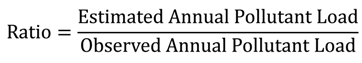
A ratio was used to compare the estimated annual pollutant loads to the observed annual pollutant loads (Equation (15)). A ratio greater than 1.0 indicates that a regression model overestimated annual pollutant load, a ratio smaller than 1.0 indicates that a regression model underestimated annual pollutant load, and a ratio of 1.0 indicates estimated annual pollutant load is the same as observed annual pollutant load.
Both accuracy and precision are critical in evaluation of regression models and sampling frequencies, because accuracy indicates the degree of systematic error and precision indicates the degree of dispersion [
26,
27]. Accuracy and precision were evaluated by comparing means of the ratio of estimate and observed annual pollutant loads and 95% confidence intervals, respectively.
3. Results and Discussion
Figure 3 shows variations of 95% confidence intervals of the ratios (Equation (15)) by different sampling frequencies and regression models of LOADIN (LD) and LOADEST (LT). The numbers with LT indicate the LOADEST model number; for instance, LT(3) indicates LOADEST model number 3. Each model in each graph has three 95% confidence intervals; the first 95% confidence interval is for the monthly (M) sampling frequency, the second 95% confidence interval is for the biweekly sampling frequency (B), and the third 95% confidence interval is for the weekly sampling frequency (W).
LOADIN and the regression models numbered 1, 3, 4, and 7 in LOADEST (LT(1), LT(3), LT(4), and LT(7) in
Figure 3a,b) were more precise for annual sediment load estimates than the regression models numbered 2, 5, 6, 8, and 9 in LOADEST (LT(2), LT(5), LT(6), LT(8), and LT(9) in
Figure 3a,b). However, mean of ratio were not much different with sampling frequencies within each regression model, which means the accuracy of regression models were similar for annual sediment load estimates (
Figure 3a,b).
A distinct feature was found in annual sediment load estimation. More frequent sampling led to accurate and less precise annual sediment load estimates with LOADEST models numbered 1, 3, 4, and 7, when comparing the weekly sampling frequency to the monthly sampling frequency (
Figure 3a,b). Nevertheless, weekly sampling data typically provided less precise (
i.e., wider 95% confidence intervals) annual sediment load estimates than monthly sampling data. Weekly sampling data with LOADEST models numbered 1, 3, 4, and 7 provided smaller differences relative to observed loads compared to monthly sampling data (
Figure 3a,b). In other words, use of frequent water quality data with LOADEST models numbered 1, 3, 4, and 7 led to the annual sediment load estimates with smaller differences compared to observed sediment load. However, use of more frequent sampling led to less accurate and less precise annual sediment load estimates with LOADEST models numbered 2, 5, 6, 8, and 9. For instance, weekly sampling frequencies with LOADEST models numbered 2, 5, 6, 8, and 9 displayed wider 95% confidence intervals than monthly sampling frequencies. Thus, it was concluded that more frequent sampling do not necessarily lead to more accurate and precise annual sediment load estimates than use of less frequent sampling.
Figure 3.
95% Confidence Intervals of Estimated to Observed Pollutant Load Ratios. (M: Monthly sampling, B: Biweekly sampling, W: Weekly sampling); (a) Sediment by Fixed Interval Sampling; (b) Sediment by Mixed Interval Sampling; (c) Phosphorus by Mixed Interval Sampling; (d) Phosphorus by Mixed Interval Sampling; (e) Nitrogen by Fixed Interval Sampling; (f) Nitrogen by Mixed Interval Sampling.
LOADIN and regression models numbered 1, 3, 4, and 7 in LOADEST provided more accurate and more precise annual phosphorus load estimates than models numbered 2, 5, 6, 8, and 9 in LOADEST with fixed interval sampling frequencies (
Figure 3c and
Table 2). Accuracy and precision were improved by including storm samples (
Figure 3c,d), this feature corresponds to the other researchers’ results [
9,
11] indicating that storm samples are important in pollutant load estimations.
In nitrogen load estimation, LOADEST provided poorer load estimates than LOADIN, and especially regression models numbered 6, 8, and 9 in LOADEST with monthly fixed sampling frequencies which were less precise than other regression models. Compared to the annual nitrogen load estimates made by LOADEST, LOADIN provided more accurate and more precise load estimates with both fixed interval sampling frequencies and mixed interval frequencies. The biweekly mixed interval sampling frequency for LOADIN displayed the most accurate and precise annual nitrogen load estimates.
The annual pollutant load estimates made by the automatic model selection of LOADEST did not provide the best precision nor accuracy for pollutant load estimation. Annual sediment and phosphorus load estimates made by regression models numbered 1, 3, 4, and 7 in LOADEST were more accurate and precise than those of the automatically selected regression model. Regression models numbered 2, 5, 6, 8, and 9 provided less precise annual sediment and phosphorus load estimates than the other regression models; however, these models were often selected by automatic model selection in LOADEST. Therefore, the annual pollutant load estimates for automatic model selection had less precision.
Pollutant regression models contain assumptions, and thus flow and water quality datasets need to match the assumptions to obtain accurate and precise pollutant load estimates. Sediment concentration data in the study matched the assumptions of LOADEST, and thus LOADEST provided more accurate and more precise pollutant load estimates than LOADIN. On the other hand, nitrogen concentration data in the study displayed a poor relationship to streamflow data. Nitrogen concentration data did not match the assumptions of LOADEST. Therefore, LOADEST is better for pollutant load estimation when flow and concentration (or load) have a strong relationship.
Table 2.
95% Confidence Intervals of Estimated to Observed Pollutant Load Ratio for Annual Phosphorus Load Estimates by Fixed Sampling.
Table 2.
95% Confidence Intervals of Estimated to Observed Pollutant Load Ratio for Annual Phosphorus Load Estimates by Fixed Sampling.
| Model | 95% Confidence Intervals of Ratios |
|---|
| Monthly fixed interval | Biweekly fixed interval | Weekly Fixed Interval |
|---|
| LD | 0.791 ± 0.016 | 0.792 ± 0.026 | 0.767 ± 0.028 |
| LT(1) | 0.828 ± 0.011 | 0.837 ± 0.014 | 0.839 ± 0.016 |
| LT(3) | 0.842 ± 0.012 | 0.854 ± 0.014 | 0.858 ± 0.016 |
| LT(4) | 0.851 ± 0.012 | 0.863 ± 0.015 | 0.868 ± 0.016 |
| LT(7) | 0.872 ± 0.013 | 0.889 ± 0.015 | 0.898 ± 0.016 |
4. Conclusions
Both streamflow and water quality data are required to compute pollutant loads. However, water quality data are typically collected less frequently than streamflow, since it is costly to collect and to analyze water quality samples. Therefore, regression models are frequently used to estimate pollutant loads from limited water quality data. LOADEST and LOADIN were evaluated with subsampled water quality datasets from daily water quality data for nitrogen, phosphorus, and sediment.
Four distinct features were observed in the study. The first feature was that more frequent sampling frequencies did not necessarily lead to more accurate and more precise annual pollutant load estimates. The second feature was that supplementing fixed interval water quality data with water quality data collected from storm events improved both accuracy and precision in annual pollutant load estimates for all water quality parameters. The third feature was that the automatic model selection in LOADEST did not necessarily lead to more accurate and precise annual pollutant load estimates. The last feature was that the behaviors of regression models were different in annual pollutant load estimation for different water quality parameters.
The study indicates that regression models numbered 1, 3, 4, and 7 in LOADEST are more accurate and precise to annual phosphorus and sediment load estimation, that the sampling frequency for phosphorus and sediment needs to include storm samples, and that LOADIN is applicable to annual nitrogen load estimation.


