Application of Set Pair Analysis-Based Similarity Forecast Model and Wavelet Denoising for Runoff Forecasting

Abstract

This study presents the application of a set pair analysis-based similarity forecast (SPA-SF) model and wavelet denoising to forecast annual runoff. The SPA-SF model was built from identical, discrepant and contrary viewpoints. The similarity between estimated and historical data can be obtained. The weighted average of the annual runoff values characterized by the highest connection coefficients was regarded as the predicted value of the estimated annual runoff. In addition, runoff time series were decomposed using wavelet transforms to acquire approximate and detailed runoff signals at various resolution levels. At each resolution level, threshold quantifications were performed by setting the values of a detailed signal below a fixed threshold to zero. The denoised runoff time series data were obtained from the approximation at the final resolution level and processed detailed signals using threshold quantification at all resolution levels of runoff by wavelet reconstruction. Instead of using the original annual runoff, the denoised annual runoff was applied to compute the similarity between estimated and historical data for model calibration. The original data were used for model calibration and validation; the denoised runoff data were used as input data to calibrate the model (obtaining different connection coefficients) that is then applied for validation purposes by using as benchmark the same original data. To verify the accuracy of the proposed method, the annual runoff data of six stations in Eastern Taiwan were analyzed. Based on a root mean square error (RMSE) criterion, the analytical results demonstrated that, for all six stations, the proposed method using denoised annual runoff outperformed the traditional SPA-SF model, using original annual runoff, because noise was effectively removed from the detailed data, using a constant threshold, thus enhancing the accuracy of the annual runoff forecasting for the SPA-SF model.

1. Introduction

Hydrological forecasts can be obtained from past observations by identifying the variation and characteristics of hydrological systems and applied for the prediction of future hydrological data. Accurate and immediate hydrological forecasting (e.g., watershed immediate flood forecasting) is essential, because it can be used as a reference for disaster decision-making. Long-term hydrological forecasting (e.g., annual runoff) can provide a critical reference for water resource planning. Many data-driven models, including linear, nonparametric or nonlinear approaches, have been developed for hydrologic discharge time series prediction in the past decades [1].

However, hydrological systems exhibit randomness, chaos, fuzziness, grayness, fractals and other uncertainties, because of the influence of human activity; therefore, the results of hydrological forecasting are typically affected by uncertainty. To reduce the uncertainty of the upcoming state of a hydrological system, it is crucial to apply the observed hydrological data and prediction theories to forecast changes in the hydrological system for a certain future period. There are many approaches to represent and quantify uncertainty, such as generalized likelihood uncertainty estimation (GLUE), probability, grey and fuzzy set theory. One of the favored methods for uncertainty assessment in rainfall-runoff modeling is GLUE. However, some fundamental questions related to the application of GLUE remain unresolved [2]. Set pair analysis (SPA) is a novel method for dealing with uncertainty problems [3]. SPA can express the overall and local structure of the relationship by using the connection degree, which can express a variety of uncertainties [3]. A hydrological time series can be effectively predicted using the SPA-based similarity forecast (SPA-SF) model proposed by Wang et al. [3]. The statistic and physical concepts of the SPA-SF model are distinctive; its computation method is visual, its precision high and its modeling scheme simple and effective [4]. Therefore, this study presents a discussion of the data-driven SPA-SF model and its application to forecasting annual runoff time series from identical, discrepant and contrary viewpoints.

The SPA theory, proposed by Zhao [5], is a novel uncertainty theory. The core of this theory is to consider certainties and uncertainties as a certain-uncertain system and to depict uniformly all types of uncertainties, such as random uncertainty, fuzzy uncertainty, indeterminate-known uncertainty, unknown and unexpected incident uncertainty and uncertainty that results from imperfect information, using a connection degree formula that can fully embody this idea [6]. SPA has been successfully applied to many fields, such as industry, agriculture, forestry, education, physical education, military affairs, traffic, data fusion, decision-making, forecasting, comprehensive evaluation and network planning [6]. In the hydrology field, the SPA-SF model has been applied to hydrological time series forecasting. Jin et al. [4] used the SPA method to compute the similarity between the estimated and historical main physical vectors from the views of identical, discrepant and contrary sides. They regarded the weighted average of values of the water resources of the historical nearest neighbor samples as the predicted value of the estimated water resources. They then established the SPA-SF model of water resources change. They observed that the statistic and physical concepts of the SPA-SF model can be applied for forecasting different hydrological time series with abundant representative historical samples.

Li and Fu [7] used the combined SPA test and correlation coefficient test to determine the primary physical vectors that determine the highest flood level, according to the unexpected flood variation process, the complex nonlinear relationship between the highest flood level and its influencing factors and extensive hazard scope. They then established the SPA-SF model of the highest flood level change. Their results also indicate that the SPA-SF model can provide a new theory for predicting the highest flood level. Wang and Li [3] introduced the basic theory of the SPA and presented the applications of the SPA in the field of water resources and hydrology. Their research targets and the contents of the SPA, as well as its key questions assist in the resolution of hydrological problems [3].

The insufficiency for annual runoff forecasting based on the SPA model is that it uses the finite-length annual runoff sequence to estimate future runoff rules; when the state of the future runoff beyond the historical data obtains the rule of itself, the model cannot do anything [8]. The annual runoff data are often affected by noise caused by sampling errors in the runoff data. The extent of the noise on the hydrological data reduces the performance of data-driven models [9]. Thus, the noise reduction of data, using an appropriate denoising scheme, may lead to an enhanced performance of the data-driven model [10]. Thus, to enhance the accuracy of runoff forecasting in the SPA-SF model, denoised annual runoff data were used to compute the similarity between estimated runoff and historical runoff samples. Wavelet analysis, a multi-resolution analysis (MRA), can effectively separate the approximate and detailed signals in original hydrological time series data. Wavelet techniques are effective for denoising, and their numerous applications include image research [11]. The wavelet denoising algorithm can satisfy the requests for various denoising procedures. Wavelet denoising is clearly superior to conventional methods and has recently been applied in the hydrology field. Lim and Lye [12] applied wavelet-based denoising to correct a series of high temporal resolution data for a streamflow, after the data had been corrupted by tidal data. Their study confirmed that there was a tidal influence at the fluvial flow gauging site. Their method also demonstrated the potential use of wavelet analysis for solving similar problems. Liu et al. [13] applied wavelet analysis to decompose runoff time series data into approximate data and detailed data. Before reconstructing the wavelet method, thresholds were added to various details to reduce noise in the original runoff data. The convergence capability, learning precision and network generalization were greatly improved in a back-propagation (BP) network model with denoised runoff data.

Wang and Fei [14] applied wavelet analysis to obtain the yearly periodic components in a data series for hydrological runoff. After eliminating periodic components, the remaining data series were denoised through wavelet analysis to obtain the dependent stochastic components. An autoregression (AR) model was then constructed using dependent stochastic series data. Their modelling results showed that, compared with traditional stochastic methods, simulation by the wavelet method obtained hydrological series parameters that were closer to those of the measured series. Wang et al. [15] indicated that, during wavelet analysis of a hydrological series, denoising methods should be used to eliminate the effects of noise. The affected range of the data of the hydrological series should be discarded before analysis, and the anomalous data should be used to highlight the actual undulation of the hydrological series. Cui et al. [16] applied the gray topological prediction method based on wavelet denoising to forecast precipitation. Their computational results showed that their model was simpler and more accurate than the basic gray topological prediction model and, therefore, provided a vital tool for forecasting precipitation, as well as preventing and mitigating disasters.

Wang et al. [17] developed a new wavelet transform method for the synthetic generation of daily stream flow sequences. The advantage of their method was that the generated sequences could capture the dependence structure and statistical properties presented in the data. Wavelet denoising could be combined with synthetic data generation. Chou [18] developed a novel framework for considering wavelet denoising in linear perturbation models (LPMs) and simple linear models (SLMs). The denoised rainfall and runoff time series data, using wavelet denoising, were applied to the SLM and regarded as the smooth seasonal mean used in the LPM. The noise (i.e., the original time series value minus the denoised time series value) was used as the perturbation term in the LPM. Chou analyzed daily rainfall-runoff data for an upstream area of the Kee-Lung River to verify the accuracy of the proposed method. He observed that wavelet denoising enhanced the rainfall-runoff modeling precision of the LPM. Li and Lu [19] applied wavelet denoising characteristics to establish the wavelet denoising SPA model. The 1959–1989 data of Fenhe reservoir Baxia station were used. Through the comparison between the single prediction model and the synthetic prediction model of hydrological forecasting and measured series, the synthetic prediction model is superior to the single prediction model.

Nejad and Nourani [10] applied the wavelet-based global soft thresholding method to denoise a daily time series of river stream discharges, observed at the outlet of the Murder Creek River at Brewton, Alabama. Thereafter, the denoised time series was applied to an artificial neural networks (ANN) model to forecast the flow discharge value on the following day. They observed that the outcome of the ANN model for streamflow forecasting could be 11% more accurate when the data were pre-processed using the wavelet-based denoising approach, compared with the results obtained using raw data. Nourani et al. [9] proposed applying the ANN approach, focusing on the wavelet-based denoising method for modeling the daily streamflow-sediment relationship. Daubechies was used as a mother wavelet to decompose both streamflow and sediment time series into detailed and approximation subseries. The appropriate input combination with raw data to estimate the current suspended sediment load (SSL) was determined and re-applied to ANN with the denoised data. Their results revealed that, regarding the determination coefficient, the result obtained using denoised data was 23.2% more accurate than that obtained using noisy, raw data. This showed that denoised data could be used successfully for ANN-based daily SSL forecasting.

Instead of using the original annual runoff time series, wavelet denoising was applied in this study to acquire the denoised annual runoff time series. Moreover, the denoised runoff time series data were applied to the SPA-SF. The uncertainty of any model mainly depends on input data, the parameters; value and the model structure. The wavelet denoising applied in the study actually reduces the uncertainty due to the input data. The remainder of this study is organized as follows. First, the structures of the SPA-SF are introduced; wavelet denoising is then described. A case study of six hydrological stations in Eastern Taiwan is introduced to demonstrate the effectiveness of the proposed method. Finally, analytical results are discussed and conclusions are given.

2. SPA-SF Model

2.1. SPA Principles

Based on a system of paired principles, Zhao [5] proposed the concept of “set pair” for the construction of SPA. “Set pair” is defined as the pair composed of two related sets in an uncertainty system [20]. For example, if the set, B_i, represents a runoff set, another runoff set is expressed by the set, B_n+1, and therefore, B_i and B_n+1 constitute a set pair. Typically, the set in the set pair analysis is expressed as H(B_i, B_n+1), which means that B_i and B_n+1 form a pair. To determine the characteristics of the set pair, identity, difference and oppositional analyses can be performed using the same, different and reverse connection degrees [20]. Constructing connection degrees and computing connection coefficients is critical for SPA and is based on the set pair.

2.2. SPA-SF Model and Its Application to Forecast Runoff

Assume the annual runoff time series with N samples are collected in the studied area, where n samples are used to establish the model (i.e., calibration), and the remaining (N-n) samples are used for forecasting (i.e., validation). The annual runoff time series can be predicted using the SPA-SF model proposed by Wang et al. [20]. Assuming a runoff time series x_i(i = 1,2,…,n), which depends on x_i-1, x_i-2,…, x_i-m+1, x_i-m, the m is the previous adjacent historical values of runoff (i.e., the most recent runoff values at the same investigated location where the forecast has to be assessed). Define the set B_i = (x_i, x_i+1,…, x_i+m−1) (i = 1,2,…,n–m), and x_m+i. are the subsequent or forecast runoff values of set B_i, as shown in Table 1 [20]. The elements of set B_i are regarded as impact factors (i.e., there are m impact factors), and x_m+i are regarded as predicted values or dependent variables. The subsequent values, x_n+1, can be predicted based on the relationship between sets B_n+1 = (x_n-m+1, x _n-m+2,…,x_n−1, x_n) and B_i, using SPA-SF [20].

The forecasting processes of the SPA-SF model are shown in Figure 1 and summarized as follows [20]:

Table 1. The sets constituted from hydrological time series [20].

Sets	Elements in sets			Subsequent values
B1	x1	x2	x3	...	xm	xm+1
B2	x2	x3	x4	...	xm+1	xm+2
B3	x3	x4	x5	...	xm+2	xm+3
...	...	...	...	...	...	...
Bn−m	xn−m	xn−m+1	xn−m+2	...	xn−1	xn
Bn+1	xn−m+1	xn−m+2	xn−m+3	...	xn	xn+1

Table 1. The sets constituted from hydrological time series [20].

Sets	Elements in sets			Subsequent values
B1	x1	x2	x3	...	xm	xm+1
B2	x2	x3	x4	...	xm+1	xm+2
B3	x3	x4	x5	...	xm+2	xm+3
...	...	...	...	...	...	...
Bn−m	xn−m	xn−m+1	xn−m+2	...	xn−1	xn
Bn+1	xn−m+1	xn−m+2	xn−m+3	...	xn	xn+1

(1)

The appropriate value of m is selected through the analysis.

(2)

Process the various elements in set B_i to obtain their symbolic rank according to certain classification criteria. Use the mean deviation to classify the elements. Calculate the average μ_j and the average absolute deviation d_j (j = 1,2…,m) of the impact factor (i.e., the same element in the set). The elements in set B_i can be classified into Classes I, II and III according to (0, μ_j − 0.5d_j), (μ_j − 0.5d_j, μ_j + 0.5d_j)and (μ_j + 0.5d_j, ∞), respectively.

Figure 1. The flowchart for the forecasting processes of the set pair analysis-based similarity forecast (SPA-SF) model.

Figure 1. The flowchart for the forecasting processes of the set pair analysis-based similarity forecast (SPA-SF) model.

(3)

Construct the current set B_{n + 1}, according to the classification standard of the quantified symbols. Construct the set pair, H(B_{n + 1,} B_i), and count the number of identical statistical symbols (i.e., identity). Count the number of statistical symbols with one difference (i.e., differences), such as Class II vs. I, or Class II vs. III. Count the number of statistical symbols with two differences (i.e., compositionality), such as Class III vs. I. Calculate the connection degree for each set pair. The connection degree μ_Bn+1~Bi, which describes the relationship between B_n+1 and B_i, is defined as [20]:

(1)

where S is the number of identities, F is the number of differences, P is the number of oppositionality and S + F + P = n. I is the uncertainty factor of the difference. The value of I is selected in the interval (−1, 1), depending on various circumstances. Occasionally, I only plays the role of a differentially labeled element. J is the antithesis coefficient; J = −1, and occasionally, J plays the role of the opposition mark.

(4)

When the values of I and J are reasonably chosen, Equation (1) becomes a value called the connection coefficient, denoted by μ′_Bn+1~Bi. In this study, the values of I and J were chosen as 0.5 and −1 [20], respectively. Thus, the connection coefficient of set pair H(B_n+1, B_i) and μ′_Bn+1~Bi can be obtained.

(5)

The K historical samples, which are the most similar to B_n+1 based on the maximum of connection coefficients μ′_Bn+1~Bi are determined. The value of K can be empirically determined or obtained from the connection coefficients that exceed a certain threshold K ≤ n^0.5. Typically, the choice of K depends on the specific circumstances of the study. In this study, the suitable value of K was chosen based on the largest values of the connection coefficients, μ′_Bn+1~Bi. The relative weights corresponding to the K historical samples can be determined from the relative membership degree, υ_n+1,i, corresponding to the connection coefficients, μ′_Bn+1~Bi. The prediction of x_n+1 can be obtained from the weighted average of the K historical samples, as follows [20]:

(2)

3. Wavelet Denoising

In practice, useful signals usually appear as low-frequency or approximate signals, whereas noise usually appears as high-frequency or detailed signals. Wavelet transforms can separate low and high frequency signals. Signals or time series data can then be decomposed according to their specific characteristics. Wavelet reconstruction can derive denoised signals from processed, decomposed signals and an approximate signal [21].

3.1. Wavelet Transforms and Daubechies Wavelet Coefficients

The discrete wavelet transform of a vector is the outcome of a linear transformation that generates a new vector of dimension equal to that of the primeval vector. This transformation, also called decomposition, can also be performed efficiently by using the Mallat MRA algorithm [22]. Two discrete filters, decomposition low-pass filter H and decomposition high-pass filter G, are needed to compute discrete wavelet transforms. This work applied the Daubechies wavelet with vanishing moment of four (DAUB4) filters proposed by Daubechies. The DAUB4 has the following four coefficients: c₀, c₁, c₂ and c₃. A decomposed matrix, F, can be applied to decompose the hydrological data vector, X, as follows [23]:

(3)

Here, a blank space represents a zero value. Equation (3) gives the one resolution level decomposition. The term “resolution level” refers to the available decomposition level for the data. Let the filter {c₀, c₁, c₂, c₃} be smoothing filter H. The odd elements of the FX output are obtained by convolving the H with the X, which gives an approximation of the original data, S. The filter {c₃, −c₂, c₁, −c₀}, denoted as G, cannot be a smoothing filter, due to its negative values. The even elements of the FX output are obtained by convolving the G with the X, which obtains W, the detailed signal for the original data [23].

To apply the features of the approximate and detailed signals, data with length N should be restructured from the approximation with length N/2 and from the detailed signal with length N/2. The transform matrix should be orthogonal, meaning that the inverse matrix of the decomposed matrix should equal the transposed matrix of the decomposed matrix. The resulting reconstruction matrix, F′, is obtained as follows [23]:

(4)

The result obtained by carrying out one-level wavelet decomposition and then carrying out reconstruction is equal to the original data, i.e., F′(FX) = X.

The coefficient values in the filter {c₀, c₁, c₂, c₃} estimated by Daubechies are as follows [23]:

(5)

3.2. Wavelet Denoising Procedure

Donoho and Johnston [24] proposed a wavelet denoising method based on thresholds for acquiring correct denoised results. This method, which is now the most common method of wavelet denoising, is performed as follows [24].

(1)

Choose an appropriate wavelet function and number of resolution level M. The original one-dimensional time series is decomposed into an approximation at resolution level M and detailed signals at various resolution levels by using wavelet transform.

(2)

Below fixed thresholds, the absolute values of detailed signals, w_j (t) (j = 1, 2,…, M), are set to zero at each resolution level. The subscript, j, represents the j-th resolution levels. The absolute values of detailed signals that exceed fixed thresholds are treated as the difference between the values of detailed signals and thresholds as follows [24].

(6)

Equation (6) gives the threshold quantifications used to obtain the processed detailed signals at each resolution level during wavelet denoising. The approximation usually does not perform threshold quantifications.

(3)

Wavelet reconstruction can derive the denoised time series data from the approximation at resolution level M and processed detailed signals (ŵ_j (t)) at all resolution levels.

4. Application and Analysis

4.1. The Proposed Method Combining SPA-SF and Wavelet Denoising

In this study, the SPA-SF model was applied to forecast annual runoff. The forecast horizon is one year. Instead of using the original annual runoff, denoised annual runoff data were used in the SPA-SF model to enhance the accuracy of the runoff forecasting. The traditional SPA-SF model can compute the similarity between the estimated runoff and historical runoff samples, from identical, discrepant and contrary viewpoints. The predictive value of the annual runoff is assumed equal to the mean of the values characterize by the highest connection coefficients [20]. To enhance the accuracy of runoff time series forecasting, denoised annual runoff data were used in this study to compute the similarity between the estimated runoff and historical runoff samples. The new weight value was obtained from the denoised annual runoff, using wavelet denoising. The new weighted average of the most similar historical annual runoff was then obtained and regarded as the new predictive value of the annual runoff. The proposed method, which combined SPA-SF and wavelet denoising, was applied to forecast the annual runoff time series. To compare the proposed wavelet denoising method with the traditional SPA-SF, only the weight values were changed in the SPA-SF for model calibration. The observed runoff data for model validation are the same for both applications with and without wavelet denoising.

In this study, the DAUB4 filter, proposed by Daubechies, was applied to decompose the annual runoff time series. Because the number of background signals was reduced to half after one resolution level wavelet decomposition and considering that the number of data was only 36, one resolution level wavelet decomposition was used in this study. Because a wavelet transform is a convoluted operation, the length of the data period may be insufficient in wavelet decomposition. If the length of the data period is insufficient, wavelet decomposition is adversely affected by the boundary effect. The 36-year duration of the data in this study circumvented the boundary effect in decomposed and restructured processes for one resolution level wavelet transforms. However, the 18-year duration of the study data in this work may have resulted in a boundary effect in decomposed and restructured processes for two resolution level wavelet transforms. Hence, the number of resolution levels in this study was chosen as one.

4.2. Determining Thresholds

In this study, the constant threshold, T, at each resolution level was determined as follows [24]:

(7)

where n_j is the length of detailed signals at each resolution level, j, and σ is the noise strength of detailed signals at each resolution level. Noise strength was obtained as follows [24]:

(8)

where w_j(t) are the detailed signals at resolution level j. The T varies according to the length of detailed signals and noise strength. The assumed error model for the choice of the error estimator in Equations (7) and (8) is Gaussian white noise with zero mean [24]. It should be noted that applying wavelet denoising based on a short time series may not provide a robust enough estimate of noise strength in Equation (8). In practice, a long time series should be used.

4.3. Collection and Collation of Research Data

In this study, the annual runoff time series of six hydrological stations in Eastern Taiwan were collected and analyzed (Table 2 and Figure 2). Eastern Taiwan is primarily composed of the cities of Hualien and Taitung. There are three major rivers and five minor rivers in Eastern Taiwan. The major rivers are Hualien, Hsiukuluan and Beinan. Most of the rivers are narrow, because of topographical constraints. The three major rivers flow from north to south and have a wide basin, because of the terrain along the East Rift Valley. The Hsiukuluan River has the biggest river basin area. The rainy season is from May to October and accounts for approximately 78% of the annual average runoff. Thirty-six annual runoff samples, from 1973 to 2008, were selected for each station. The annual runoff of the first 30 years was used to build the SPA-SF model for calibration, and the annual runoff of the remaining six years was used to forecast the annual runoff for validation.

Table 2. The information of six hydrological stations in Eastern Taiwan.

Name of stations	Name of rivers	Name of river basins	Drainage basin area (km2)
Lijia	Lijia River	Lijia River	148.62
Yanping	Kano River	Beinan River	476.16
Tateyama	Fung Ping River	Hsiukuluan River	249.40
Mizuho Bridge	Hsiukuluan River	Hsiukuluan River	1538.81
Renshou Bridge	Mugua River	Hualien River	425.92
Hualien Bridge	Hualien River	Hualien River	1506.00

Table 2. The information of six hydrological stations in Eastern Taiwan.

Name of stations	Name of rivers	Name of river basins	Drainage basin area (km2)
Lijia	Lijia River	Lijia River	148.62
Yanping	Kano River	Beinan River	476.16
Tateyama	Fung Ping River	Hsiukuluan River	249.40
Mizuho Bridge	Hsiukuluan River	Hsiukuluan River	1538.81
Renshou Bridge	Mugua River	Hualien River	425.92
Hualien Bridge	Hualien River	Hualien River	1506.00

Figure 2. The location of the six investigated hydrometric sites in eastern Taiwan. The boundaries of the drainage basins are also shown [25]. (a) Lijia Station; (b) Yanping Station; (c) Tateyama and Mizuho Bridge Station; (d) Renshou Bridge and Hualien Bridge Station.

Figure 2. The location of the six investigated hydrometric sites in eastern Taiwan. The boundaries of the drainage basins are also shown [25]. (a) Lijia Station; (b) Yanping Station; (c) Tateyama and Mizuho Bridge Station; (d) Renshou Bridge and Hualien Bridge Station.

4.4. Comparison of Models

To compare the results obtained using denoised runoff with those using the original runoff in the SPA-SF model, the root mean square error (RMSE) was used in this study and was defined as follows:

(9)

where Ԛ_est and Ԛ_obs represent the estimated and observed runoff, respectively. A small RMSE value indicates that the simulation results were close to the actual data and had high accuracy.

5. Results and Discussion

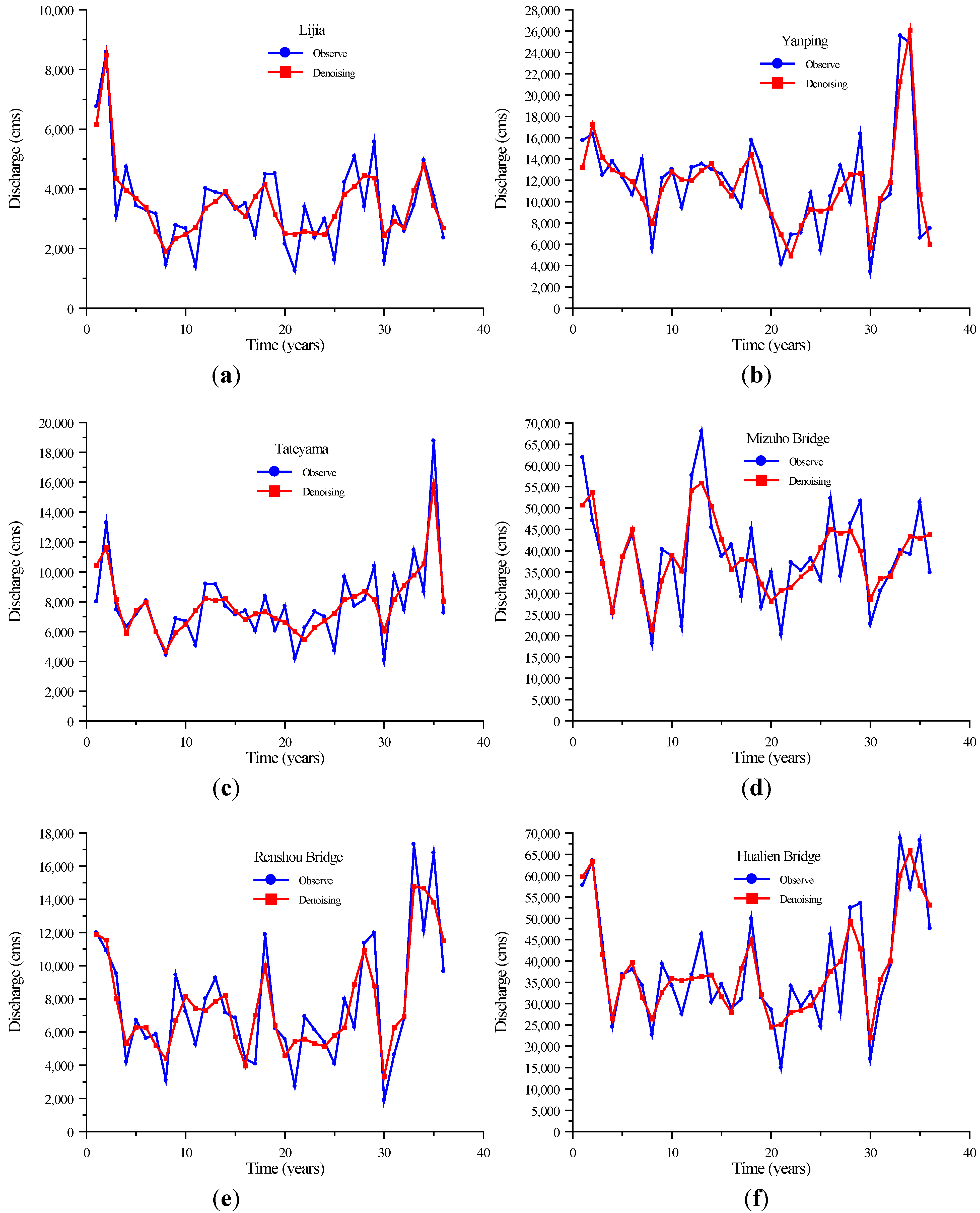
The wavelet denoising method using a fixed threshold denoising, proposed by Donoho [24], was applied to the annual runoff time series. The original time series of the annual runoff and the denoised annual runoff time series of the six stations are shown in Figure 3. When the traditional denoising algorithm (e.g., Fourier filtering) is applied, data distortion is generated, and the true meaning of the data is lost. Figure 3 shows that the wavelet denoising method exerted a smoothing effect, and the data had little distortion. This result suggests that the wavelet denoising method can be used for different denoising technique requests and has prime advantages compared with the traditional denoising method (e.g., Fourier filtering).

Figure 3. Original annual runoff time series and denoised annual runoff time series using wavelet denoising of the six stations. (a) Lijia Station; (b) Yanping Station; (c) Tateyama Station; (d) Mizuho Bridge Station; (e) Renshou Bridge Station; (f) Hualien Bridge Station.

Figure 3. Original annual runoff time series and denoised annual runoff time series using wavelet denoising of the six stations. (a) Lijia Station; (b) Yanping Station; (c) Tateyama Station; (d) Mizuho Bridge Station; (e) Renshou Bridge Station; (f) Hualien Bridge Station.

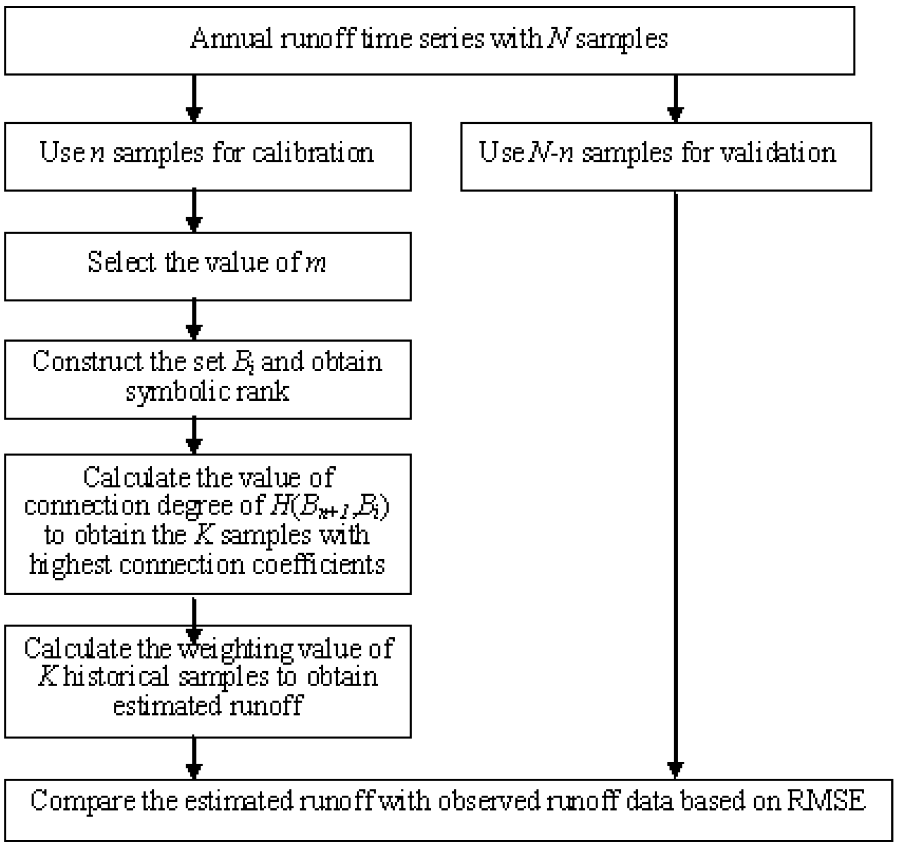
In this study, the SPA-SF model was applied to forecast an annual runoff time series. The value of m was selected to be five through the analysis [20], that is the runoff time series x_i(i = 1,2,…,n) was dependent on the five previous historical values. With a certain classification criteria, the various elements in set B_i were processed to obtain the symbolic rank. The current set B_{n + 1} was constructed and quantified according to the classification standard symbols. In addition, the values of I and J were selected as 0.5 and −1 [20], respectively. The connection coefficient, μ′_Bn+1~Bi, of the set pair, H(B_n+1, B_i), was then obtained. A suitable value of K was chosen based on the number of the largest contact coefficients, μ′_Bn+1~Bi. Equation (2) was used to forecast the annual runoff time series. For example, the calculation process for the Hualien Bridge station in 2003 is shown in Table 3. Table 3 shows that the values of the largest connection coefficient and K were 0.8 and 2, respectively. These data indicate that the values of the largest connection coefficient and K were reasonable. This result suggests that the SPA-SF model can be applied to forecast annual runoff time series.

Table 3. The calculation process of forecasting annual runoff for the Hualien Bridge station in 2003.

Sets	xi	xi+1	xi+2	xi+3	xi+4	Subsequent values xi+5	Identity	Differences	Compositionality	Connection coefficients
B1	III	III	III	I	II	37,977	0.4	0.2	0.4	0.1
B2	III	III	I	II	II	34,293	0.2	0.4	0.4	0.0
B3	III	I	II	III	II	22,702	0.6	0.4	0.0	0.8
B4	I	II	III	II	I	39,307	0.4	0.4	0.2	0.4
B5	II	II	II	I	II	34,200	0.0	0.8	0.2	0.2
B6	II	II	I	I	II	27,551	0.2	0.6	0.2	0.3
B7	II	I	III	II	I	36,767	0.6	0.4	0.0	0.8
B8	I	II	II	I	II	46,204	0.0	0.6	0.4	-0.1
B9	II	II	I	II	III	30,304	0.0	0.6	0.4	-0.1
B10	II	I	II	III	II	34,553	0.4	0.6	0.0	0.7
B11	I	II	III	II	II	28,901	0.2	0.6	0.2	0.3
B12	II	III	II	II	I	31,007	0.2	0.6	0.2	0.3
B13	III	II	II	I	II	49,942	0.2	0.6	0.2	0.3
B14	II	II	I	II	III	31,395	0.0	0.6	0.4	−0.1
B15	II	I	II	III	II	28,567	0.4	0.6	0.0	0.7
B16	I	II	III	II	I	14,963	0.4	0.4	0.2	0.4
B17	II	III	II	I	I	34,098	0.2	0.4	0.4	0.0
B18	III	II	I	I	II	29,349	0.2	0.4	0.4	0.0
B19	II	I	I	II	I	32,706	0.4	0.4	0.2	0.4
B20	I	I	II	II	II	24,671	0.2	0.6	0.2	0.3
B21	I	II	II	II	I	46,275	0.2	0.6	0.2	0.3
B22	II	I	II	I	III	28,012	0.2	0.4	0.4	0.0
B23	I	II	I	III	I	52,494	0.4	0.2	0.4	0.1
B24	II	I	III	I	III	53,543	0.4	0.2	0.4	0.1
B25	I	III	I	III	III	16,919	0.2	0.0	0.8	−0.6
B26	III	I	III	III	I	–	–	–	–	–

Table 3. The calculation process of forecasting annual runoff for the Hualien Bridge station in 2003.

Sets	xi	xi+1	xi+2	xi+3	xi+4	Subsequent values xi+5	Identity	Differences	Compositionality	Connection coefficients
B1	III	III	III	I	II	37,977	0.4	0.2	0.4	0.1
B2	III	III	I	II	II	34,293	0.2	0.4	0.4	0.0
B3	III	I	II	III	II	22,702	0.6	0.4	0.0	0.8
B4	I	II	III	II	I	39,307	0.4	0.4	0.2	0.4
B5	II	II	II	I	II	34,200	0.0	0.8	0.2	0.2
B6	II	II	I	I	II	27,551	0.2	0.6	0.2	0.3
B7	II	I	III	II	I	36,767	0.6	0.4	0.0	0.8
B8	I	II	II	I	II	46,204	0.0	0.6	0.4	-0.1
B9	II	II	I	II	III	30,304	0.0	0.6	0.4	-0.1
B10	II	I	II	III	II	34,553	0.4	0.6	0.0	0.7
B11	I	II	III	II	II	28,901	0.2	0.6	0.2	0.3
B12	II	III	II	II	I	31,007	0.2	0.6	0.2	0.3
B13	III	II	II	I	II	49,942	0.2	0.6	0.2	0.3
B14	II	II	I	II	III	31,395	0.0	0.6	0.4	−0.1
B15	II	I	II	III	II	28,567	0.4	0.6	0.0	0.7
B16	I	II	III	II	I	14,963	0.4	0.4	0.2	0.4
B17	II	III	II	I	I	34,098	0.2	0.4	0.4	0.0
B18	III	II	I	I	II	29,349	0.2	0.4	0.4	0.0
B19	II	I	I	II	I	32,706	0.4	0.4	0.2	0.4
B20	I	I	II	II	II	24,671	0.2	0.6	0.2	0.3
B21	I	II	II	II	I	46,275	0.2	0.6	0.2	0.3
B22	II	I	II	I	III	28,012	0.2	0.4	0.4	0.0
B23	I	II	I	III	I	52,494	0.4	0.2	0.4	0.1
B24	II	I	III	I	III	53,543	0.4	0.2	0.4	0.1
B25	I	III	I	III	III	16,919	0.2	0.0	0.8	−0.6
B26	III	I	III	III	I	–	–	–	–	–

The results that were obtained by applying the traditional SPA-SF model to annual runoff time series forecasting are denoted as SPA-SF (Table 4). By contrast, the results that combined the SPA-SF model and wavelet denoising are denoted as SPA-SFW (Table 4). To compare the SPA-SF with SPA-SFW, only the similarity between estimated and historical runoff data (i.e., weights in Equation (2)) were changed. The predicted value of the estimated annual runoff was obtained from the weighted average of the non-denoised annual runoff of the nearest neighbor historical samples. Table 4 shows that, based on RMSE, the results obtained using the SPA-SFW model were better than those obtained using the SPA-SF model, for all six stations.

Table 4. The forecasting results obtained using the SPA-SF and SPA-SF model and wavelet denoising (SPA-SFW) based on the RMSE for six stations.

Lijia				Yanping
Year	Observe (m3/s)	SPA-SF (m3/s)	SPA-SFW (m3/s)	Year	Observe (m3/s)	SPA-SF (m3/s)	SPA-SFW (m3/s)
2003	3,385	3,051	2,192	2003	9,928	8,174	9,844
2004	2,587	2,774	2,920	2004	10,674	14,195	9,477
2005	3,448	2,890	2,789	2005	25,568	7,635	11,234
2006	4,954	3,880	4,492	2006	24,889	13,261	13,037
2007	3,757	2,943	4,029	2007	6,589	8,547	8,487
2008	2,357	3,124	2,151	2008	7,510	4,147	9,844
RMSE		691	619	RMSE		9,013	7,707
Tateyama				Mizuho Bridge
Year	Observe (m3/s)	SPA-SF (m3/s)	SPA-SFW (m3/s)	Year	Observe (m3/s)	SPA-SF (m3/s)	SPA-SFW (m3/s)
2003	9,730	6,403	6,725	2003	30,552	34,723	34,158
2004	7,455	6,901	7,117	2004	34,808	38,753	32,795
2005	11,458	8,154	7,047	2005	40,134	38,702	37,280
2006	8,664	8,207	8,765	2006	39,159	32,655	45,371
2007	18,772	5,639	7,411	2007	51,320	44,931	52,029
2008	7,257	8,207	6,939	2008	34,877	51,015	42,048
RMSE		5,713	5,128	RMSE		7,943	4,391
Renshou Bridge						Hualien Bridge
Year	Observe (m3/s)	SPA-SF (m3/s)	SPA-SFW (m3/s)	Year	Observe (m3/s)	SPA-SF (m3/s)	SPA-SFW (m3/s)
2003	4,624	7,428	4,225	2003	31,077	29,734	31,007
2004	6,783	4,851	5,628	2004	38,921	37,552	36,088
2005	17,327	6,896	7,834	2005	68,780	34,293	34,293
2006	12,114	5,135	5737	2006	57,138	28,371	29,611
2007	16,804	11,979	11,979	2007	68,247	28,901	34,707
2008	9,657	6,939	7,166	2008	47,589	30,673	41,024
RMSE		5,770	5,192	RMSE		25,347	22,815

Table 4. The forecasting results obtained using the SPA-SF and SPA-SF model and wavelet denoising (SPA-SFW) based on the RMSE for six stations.

Lijia				Yanping
Year	Observe (m3/s)	SPA-SF (m3/s)	SPA-SFW (m3/s)	Year	Observe (m3/s)	SPA-SF (m3/s)	SPA-SFW (m3/s)
2003	3,385	3,051	2,192	2003	9,928	8,174	9,844
2004	2,587	2,774	2,920	2004	10,674	14,195	9,477
2005	3,448	2,890	2,789	2005	25,568	7,635	11,234
2006	4,954	3,880	4,492	2006	24,889	13,261	13,037
2007	3,757	2,943	4,029	2007	6,589	8,547	8,487
2008	2,357	3,124	2,151	2008	7,510	4,147	9,844
RMSE		691	619	RMSE		9,013	7,707
Tateyama				Mizuho Bridge
Year	Observe (m3/s)	SPA-SF (m3/s)	SPA-SFW (m3/s)	Year	Observe (m3/s)	SPA-SF (m3/s)	SPA-SFW (m3/s)
2003	9,730	6,403	6,725	2003	30,552	34,723	34,158
2004	7,455	6,901	7,117	2004	34,808	38,753	32,795
2005	11,458	8,154	7,047	2005	40,134	38,702	37,280
2006	8,664	8,207	8,765	2006	39,159	32,655	45,371
2007	18,772	5,639	7,411	2007	51,320	44,931	52,029
2008	7,257	8,207	6,939	2008	34,877	51,015	42,048
RMSE		5,713	5,128	RMSE		7,943	4,391
Renshou Bridge						Hualien Bridge
Year	Observe (m3/s)	SPA-SF (m3/s)	SPA-SFW (m3/s)	Year	Observe (m3/s)	SPA-SF (m3/s)	SPA-SFW (m3/s)
2003	4,624	7,428	4,225	2003	31,077	29,734	31,007
2004	6,783	4,851	5,628	2004	38,921	37,552	36,088
2005	17,327	6,896	7,834	2005	68,780	34,293	34,293
2006	12,114	5,135	5737	2006	57,138	28,371	29,611
2007	16,804	11,979	11,979	2007	68,247	28,901	34,707
2008	9,657	6,939	7,166	2008	47,589	30,673	41,024
RMSE		5,770	5,192	RMSE		25,347	22,815

The overall comparisons between SPA-SF and SPA-SFW, using the RMSE for six stations, are shown in Table 5. Based on the RMSE, the average value of the SPA-SFW (7642) model was better than that of the SPA-SF (9080) model, as shown in Table 5. These results imply that using a denoised annual runoff time series for the SPA-SF model allows an accurate computing of the similarity between the estimated runoff and historical runoff data. Hence, better weighted values could be obtained using denoised runoff data. Moreover, the weighted average of the most similar historical runoff samples resulted in a more accurate forecasting of runoff than that obtained using the original runoff data in the SPA-SF model. This was because the high frequency and low frequency components of the signals could be effectively separated by wavelet decomposition. In addition, the high frequency components of the signals could be denoised using threshold quantifications. The denoised annual runoff was used to accurately compute the similarity between estimated and historical data in the SPA-SF model, enhancing the accuracy of runoff forecasting. The values of coefficients S/m, F/m and P/m in Equation (1) are different for SPA-SF and SPA-SFW. The values of these coefficients in the SPA-SF and SPA-SFW models are obtained from original and denoised annual runoff data, respectively. The noise reduction of data, using wavelet denoising, leads to an enhanced performance of the proposed data-driven model. This is the reason why SPA-SFW outperforms SPA-SF based on the SPA analysis model of Equation (1).

Table 5. The average forecasting results obtained using SPA-SF, SPA-SFW and autoregression (AR) based on RMSE.

Name of stations	SPA-SF	SPA-SFW	AR
Lijia	691	619	1,061
Yanping	9,013	7,707	9,141
Tateyama	5,713	5,128	4,674
Mizuho Bridge	7,943	4,391	9,030
Renshou Bridge	5,770	5,192	6,036
Hualien Bridge	25,347	22,815	21,146
Average	9,080	7,642	8,515

Table 5. The average forecasting results obtained using SPA-SF, SPA-SFW and autoregression (AR) based on RMSE.

Name of stations	SPA-SF	SPA-SFW	AR
Lijia	691	619	1,061
Yanping	9,013	7,707	9,141
Tateyama	5,713	5,128	4,674
Mizuho Bridge	7,943	4,391	9,030
Renshou Bridge	5,770	5,192	6,036
Hualien Bridge	25,347	22,815	21,146
Average	9,080	7,642	8,515

To compare the results obtained using the proposed method with the results obtained using the traditional method, the AR model was applied to annual runoff forecasting. The validated results obtained using SPA-SF and SPA-SFW were compared with the results obtained via the auto regressive (AR) model, as shown in Table 5. For consistency, the value of m for AR model was selected to be five. The values of the calibrated coefficients in the AR model for six stations are shown in Table 6. Based on the RMSE, the average value of the SPA-SF (9080) was higher than that of the AR (8515). However, the average value of the SPA-SFW (7642) was lower than that of the AR (8515). It can be seen that the SPA-SFW (7642) outperforms AR (8515) and the SPA-SF (9080) based on the RMSE.

Table 6. The values of the calibrated coefficients in the AR model for six stations.

Name of stations	m = 1	m = 2	m = 3	m = 4	m = 5
Lijia	0.31699	0.25847	0.25648	−0.03414	0.13865
Yanping	0.22231	0.26237	0.15771	−0.14061	0.43697
Tateyama	0.08698	0.30733	0.47995	0.11940	−0.00456
Mizuho Bridge	0.31934	0.13720	0.39881	0.18277	−0.05631
Renshou Bridge	0.21177	0.09370	0.22852	0.28814	0.14405
Hualien Bridge	0.06826	0.21847	0.36847	0.20636	0.12162

Table 6. The values of the calibrated coefficients in the AR model for six stations.

Name of stations	m = 1	m = 2	m = 3	m = 4	m = 5
Lijia	0.31699	0.25847	0.25648	−0.03414	0.13865
Yanping	0.22231	0.26237	0.15771	−0.14061	0.43697
Tateyama	0.08698	0.30733	0.47995	0.11940	−0.00456
Mizuho Bridge	0.31934	0.13720	0.39881	0.18277	−0.05631
Renshou Bridge	0.21177	0.09370	0.22852	0.28814	0.14405
Hualien Bridge	0.06826	0.21847	0.36847	0.20636	0.12162

Because the SPA-SF model refers to historical samples to predict runoff, outliers that are substantially different from the historical minimum or maximum could result in poor predictive results. In other words, the size of the historical samples affects the predictive results obtained in the SPA-SF model. When the representativeness of the historical samples is high, it is expected to obtain reasonable and reliable predictions. In addition, the resolution level of the wavelet decomposition is also related to the size of the historical samples.

6. Conclusions

In this study, the SPA-SF model and wavelet denoising were applied to forecast annual runoff. The annual runoff data are often affected by noise, which reduces the performance of data-driven models. The similarity between estimated and historical runoff data in the SPA-SF model was computed from identical, discrepant and contrary viewpoints. Instead of using the original annual runoff, the denoised annual runoff using wavelet denoising was applied to compute the similarity between estimated and historical data more accurately than did the traditional SPA-SF model using the original annual runoff for model calibration. The estimated annual runoff is assumed equal to the weighted average of the values characterized by the highest connection coefficients. Therefore, the noise reduction of data through wavelet denoising led to an enhanced performance of the proposed data-driven model.

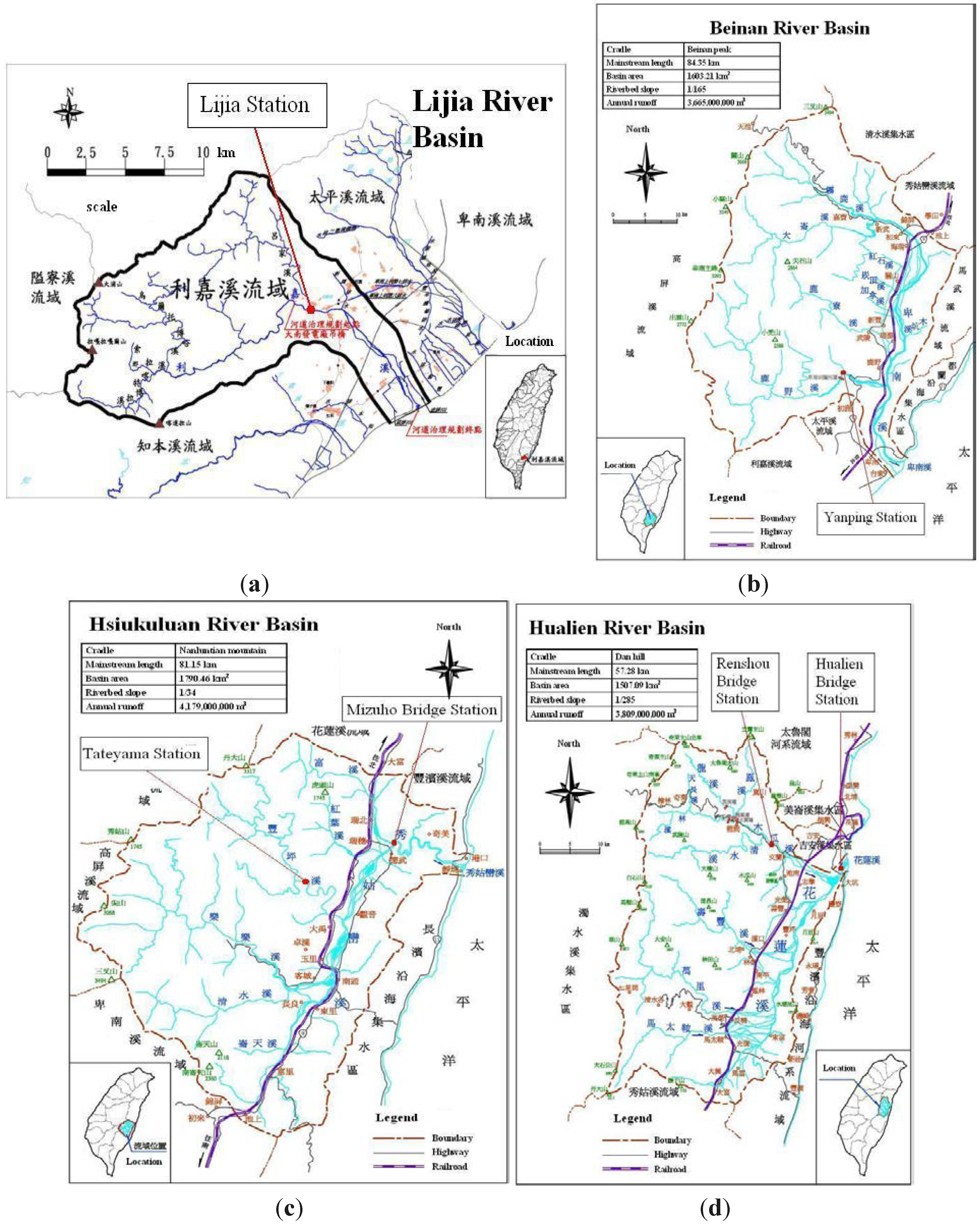
The annual runoff data of six stations in Eastern Taiwan were analyzed to verify the accuracy of the proposed method. The observed runoff data used as a benchmark for model validation purposes are the same for both applications with and without wavelet denoising. In this study, the results obtained using the annual runoff, with and without wavelet denoising, were compared. For the data obtained from the historical samples, the SPA-SFW model obtained smaller values based on the RMSE, compared with those obtained using the SPA-SF and AR model. Considering the length of the data, one resolution level was applied to carry out wavelet decomposition and denoising, obtaining acceptable results when compared with the SPA-SF and AR model based on the RMSE. The obtained results are encouraging, but further analyses on different case studies should be carried out, and some specific hydrological understanding should be added to confirm the usefulness of the proposed method for water resources planning activities.