Article

Self-Powered Desalination of Geothermal Saline Groundwater: Technical Feasibility

1
Sustainable Environment Research Group, School of Engineering and Applied Science, Aston University, Birmingham B4 7ET, UK
2
Department of Mechanical Engineering, College of Engineering, King Saud University, PO Box 800, Riyadh 11421, Saudi Arabia
*
Author to whom correspondence should be addressed.
Water 2014, 6(11), 3409-3432; https://doi.org/10.3390/w6113409
Submission received: 11 July 2014 / Revised: 16 October 2014 / Accepted: 22 October 2014 / Published: 12 November 2014

Abstract

:
This theoretical study shows the technical feasibility of self-powered geothermal desalination of groundwater sources at <100 °C. A general method and framework are developed and then applied to specific case studies. First, the analysis considers an ideal limit to performance based on exergy analysis using generalised idealised assumptions. This thermodynamic limit applies to any type of process technology. Then, the analysis focuses specifically on the Organic Rankine Cycle (ORC) driving Reverse Osmosis (RO), as these are among the most mature and efficient applicable technologies. Important dimensionless parameters are calculated for the ideal case of the self-powered arrangement and semi-ideal case where only essential losses dependent on the RO system configuration are considered. These parameters are used to compare the performance of desalination systems using ORC-RO under ideal, semi-ideal and real assumptions for four case studies relating to geothermal sources located in India, Saudi Arabia, Tunisia and Turkey. The overall system recovery ratio (the key performance measure for the self-powered process) depends strongly on the geothermal source temperature. It can be as high as 91.5% for a hot spring emerging at 96 °C with a salinity of 1830 mg/kg.

1. Introduction

Exploitation of geothermal energy for power generation is a mature field, with many plants operating for example in Iceland, Japan, Italy and elsewhere [1,2]. Lund et al. [1] reviewed the worldwide application of geothermal energy for direct utilization. Data and information on geothermal utilization corresponding to about 80 countries were screened and presented. The worldwide installed thermal power for direct utilization was estimated to be 48.49 GWt at the end of 2009.
In contrast, the use of geothermal energy specifically for desalination is a relatively unexplored topic, with only a few studies done. The earliest work seems to be that of Awerbuch et al. [3] who in 1976 proposed and analysed a novel process for the production of power and water from geothermal brines. The process consisted of a separator, steam turbine and a multi-stage flash (MSF) distiller. The separator ensured that just distilled steam—flashed from the hot brine from the production well—circulated in the steam turbine; while the non-evaporated water fed the MSF unit. More recently, Bourouni et al. [4], and subsequently Mohamed and El Minshawy [5], conducted theoretical and experimental studies on desalting water using humidification-dehumidification processes in Tunisia and Egypt respectively. Mahmoudi et al. [6] proposed a new brackish water greenhouse desalination unit powered by geothermal energy for the development of arid and relatively cold regions, using Algeria as a case study. This process was also based on the humidification and dehumidification of air. The authors reported that brackish water desalination is one of the most promising fields of application of geothermal energy. Bouguecha and Dhabi [7] conducted an experimental study using a fluidized bed crystalliser and air gap membrane distillation driven by geothermal energy. Mathioulakis et al. [8], in their review of desalination using alternative energy, claimed that geothermal energy presents a mature technology that can be used to drive desalination at competitive costs. Recently, Koroneos and Roumbas [9] studied the possibility of utilizing the existing geothermal potential on the Greek island of Nisyros for water desalination. They developed a simple model based on exergy analysis for a multiple effect distillation unit driven by geothermal energy and found that the exergy destruction rate was 48.6%.
Reverse osmosis (RO) driven by the organic Rankine cycle (ORC) is the most promising and efficient method of desalination where the thermal energy source is limited in supply and at low temperature. The low boiling point of organic fluids allows conversion of heat to power in a compact machine. The use of ORC in various applications has been considered in a number of recent studies. For example, Li et al. [10] proposed and analysed the performance of a RO desalination process powered by supercritical ORC with a source temperature limited to 150 °C. Manlolakos et al. [11] designed, built and tested a solar-powered ORC for desalination of seawater using the working fluid R134a. Igobo and Davies [12] developed an isothermal version of the ORC for use with a batch desalination process and, based on experiments with R245fa, predicted a specific energy thermal consumption of 2.5 kWh/m3 at evaporator temperature of 90 °C in desalination of brackish water containing 4000 mg kg−1 NaCl at 70% recovery. A number of exergy studies have been carried out for ORC [13,14] and for RO separately [15,16], but relatively few for ORC coupled to RO [17,18].
Several arid countries benefit from geothermal resources including Australia, Algeria, Saudi Arabia, Tunisia, US, and regions of India [1]. In some locations, geothermal activity coincides with saline aquifers but the extent of this coincidence is not yet thoroughly studied or mapped extensively. Specific locations where these resources coincide include the Kebili Aquifer (Tunisia), the Najd Plateau (Saudi Arabia), Gujarat (India) and the Kütahya-Simav geothermal field (Turkey). It is likely that with increased interest in geothermal desalination and with further exploration, an increasing number of relevant sites will be discovered.
At some sites, saline aquifers are exploited for water while their geothermal energy is neglected. In the Salbukh region of Riyadh in Saudi Arabia, for example, saline water is passed through cooling towers before being supplied to RO plant which is powered by grid electricity. Not only is this a waste of geothermal energy that could be harnessed; it also requires significant infrastructure investment to supply electricity to an outlying location.
To take advantage of such resources, this study aims to determine the technical feasibility of self-powered geothermal desalination. “Self-powered” means that all the energy requirements for the desalination process are obtained from the heat of the feed water. The theory in Section 2.1 considers an ideal limit to performance based on an exergy analysis using generalized assumptions. This thermodynamic limit applies to any type of process technology. Then, in Sections 2.2 and Section 2.3, the analysis is focused specifically on RO and ORC technologies respectively. Progressively more realistic assumptions are then introduced to predict the maximum possible performance using specific plant configurations. In Section 3, four case studies are introduced, with results given in Section 4. Though this paper deals mainly with technical aspects of the plant design at the concept level, some preliminary discussion is also given to the economic and detailed engineering aspects of the design, including pre- and post-treatment (Section 5). Section 6 concludes the study.

2. Theory

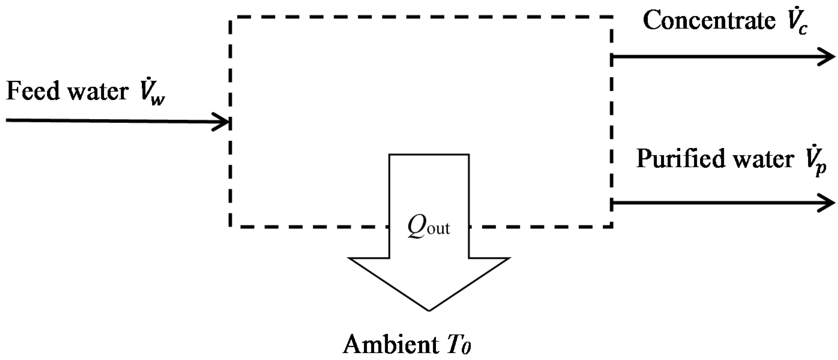
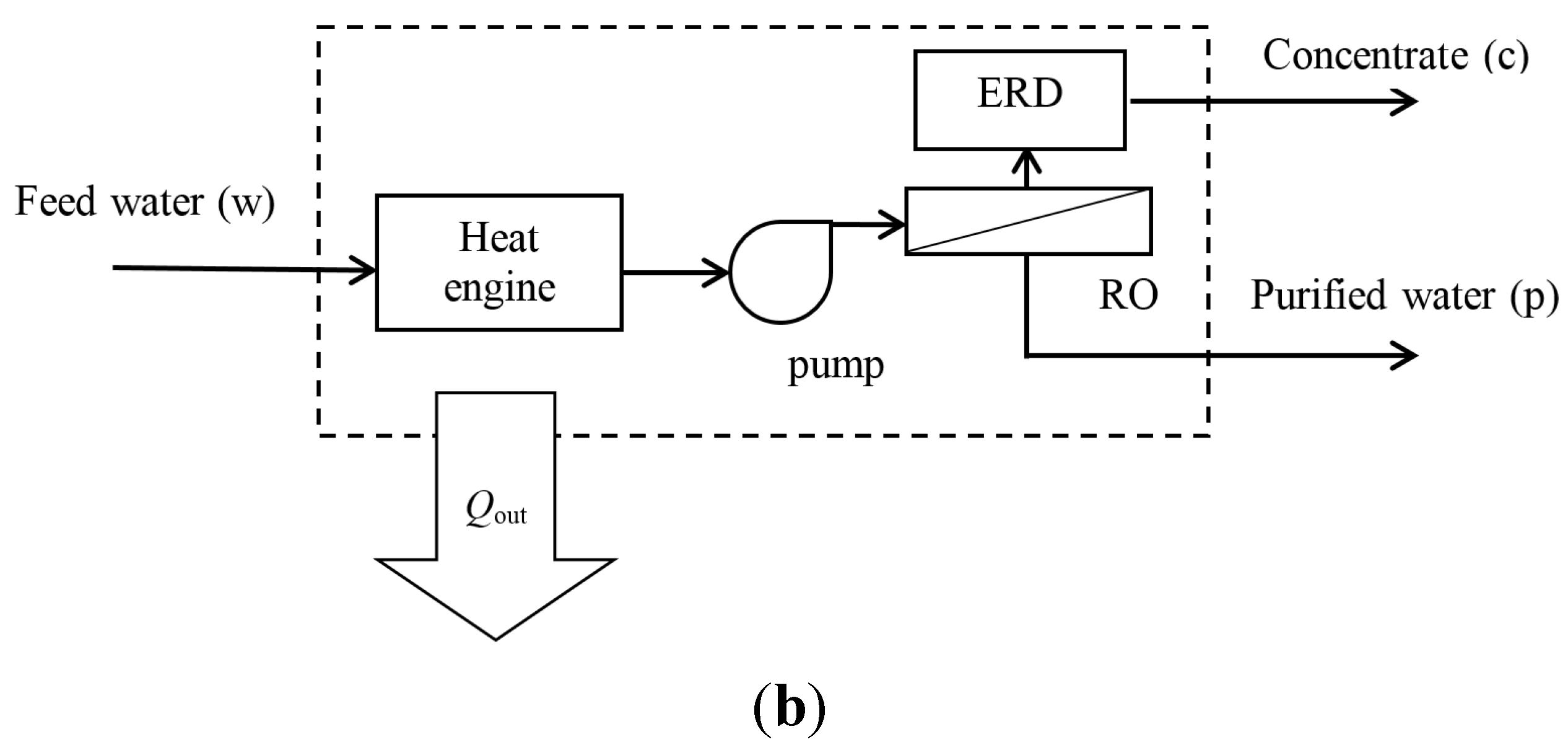
2.1. Exergy Analysis

A generalized concept of the geothermal-powered desalination plant is presented as a control volume (Figure 1) which incorporates all the energy conversion and desalination equipment needed to separate the saline feed water into two outputs: more saline concentrate and non-saline purified water. In this paper, the equipment consists of a heat engine together with a RO process; however, the exergy analysis would apply equally well to other processes to determine an upper limit to performance based on the 2nd law of thermodynamics.
The aim of the process is to maximise the output of purified water V ˙ p (m3/s) for a given flow V ˙ w of feed water taken from the geothermal source; therefore the performance will be quantified as the overall recovery ratio of the system defined by:
r s y s   =   V ˙ p V ˙ w
We are interested to determine the maximum possible value of rsys. Further parameters could be introduced to describe the quality (and not just quantity) of the water output, but these are not considered at the stage of the exergy analysis.
Figure 1. Self-powered geothermal desalination plant represented as a control volume that includes geothermal energy conversion and desalination equipment.
Water 06 03409 g001
The separation requires work that is obtained purely from the thermal energy of the feed water which is supplied at a temperature Tw above ambient. The system rejects heat to the surroundings, at ambient temperature T0, such that the two streams exit at lower temperatures than that of the feed. There is no work input from the surroundings—the only work transfer will be internal to the system. The intention of the exergy analysis is to provide a preliminary and general indication of the theoretical scope for the self-powered separation using analytical expressions. At this initial stage, a highly accurate result is not sought because it is anticipated that the real performance will in any case be much less than the ideal one. Accordingly, the analysis will be simplified by a number of idealised assumptions and approximations as follows:
  • The purified water is free of salt i.e., the rejection fraction is 100%. Indeed, most modern desalination technologies typically achieve rejection fractions well above 95%. This assumption is conservative, in that lower rejection fractions will generally require less energy, so the separation will be accomplished more readily.
  • The energy consumptions of auxiliary processes (e.g., pre-treatment and post-treatment) are not considered. Due to the varied nature of these processes, however, they are not amenable to a generalised thermodynamic analysis. (In practice, auxiliary processes are important and these will later be discussed in outline in relation to specific case studies).
  • Similarly, energy needed to lift the water from the source, and potential or kinetic energy associated with the pressure of the source water, are neglected.
  • Assumptions valid for dilute solutions are used: the density and specific heat capacity are considered independent of concentration, and osmotic pressure is considered proportional to the molar concentration of salt. This is justified by the fact that groundwater sources studied here have salt concentrations <10,000 mg/kg.
The maximum possible work W ˙ t that can be harnessed from the geothermal energy of the feed is given by the widely-used exergy expression [19]:
W ˙ t   =   ( H ˙ w H ˙ * ) T 0 ( S ˙ w S ˙ * )
where H ˙ indicates the enthalpy flow (kJ s−1); and S ˙ the entropy flow (kJ K−1 s−1). The superscript * refers to the thermal (i.e., restricted) dead state obtained when the water is brought to the ambient temperature T0 and pressure P0 without change in concentration. For a process assumed to have unchanged pressure between inlet and outlet:
W ˙ t   =   m ˙ w c p [ ( T w T 0 ) T 0 ln ( T w T 0 ) ]
The work will be used to carry out the desalination process within the control volume with no external exchange of work.
The minimum work of desalination has been studied by several authors using models of varying complexity to represent solution properties with focus on the properties of concentrated seawater [20,21,22]. Here, a more simple approach is adopted justified by the fact that the feed solution is very dilute. Hence the osmotic pressure Posm is assumed to follow the van’t Hoff relation:
P o s m V   =   n R T 0
where n (kmol) is the number of moles of solute in the volume V. Note that Equation (4) applies not only to solutions containing a single salt but also to mixed solutions, as n can represent the effective sum over all salt species present. The calculation of osmotic pressure Posm also takes into account the dissociation of the salts present and experimentally determined values of osmotic coefficient, as detailed in the Appendix.
The expression for the ideal minimum specific energy consumption of desalination at recovery r, based on the van’t Hoff expression, has been given elsewhere as [23]:
SEC i d e a l   =   P o s m 1 r ln ( 1 1 r )
The minimum rate of work needed for the system will therefore be:
W ˙ s   =   P o s m V w ̇ ln ( 1 1 r )
In the ideal self-powered system, the separation process receives work input only from the conversion of the geothermal energy such that   W ˙ s   =   W ˙ t . Thus:
P o s m V w ̇ ln ( 1 1 r s y s )   =   m ˙ w c p [ ( T w T 0 ) T 0 ln ( T w T 0 ) ]
Re-arrangement gives an expression for the maximum recovery rate rsys achievable based on the exergy consideration:
r s y s   =   1 e A
where
A   =   ρ c p P o s m [ ( T w T 0 ) T 0 ln ( T w T 0 ) ]
The dimensionless parameter A quantifies the amount of thermo-mechanical work available relative to the theoretical minimum work of desalination as recovery nears zero. A high value of A indicates the self-powered separation should be relatively easy to accomplish enabling a high possible value of rsys. Thus, at A = 2.3, rsys could be as high as 0.9 in principle, which would usually be considered a very good recovery ratio for a desalination process because only 10% of the feedwater is wasted. To give a preliminary practical example, this value of A = 2.3 would be achieved with a feed temperature of just Tw = 57 °C at ambient conditions T0 = 40 °C and saline water with Posm = 800 kPa, corresponding to NaCl solution of concentration about 10,000 mg kg−1. The exergy analysis thus reveals plenty of scope for the self-powered desalination process even with low temperature sources.
Note that the Equation (8), subject to the assumptions listed above, describes a general upper limit not just for RO but for any process having the same inlet and outlet conditions. This is because the RO process is, in the limit considered, thermodynamically reversible. Thus, other processes (e.g., electrodialysis or capacitive discharge ionization) are subject to the same limiting value of rsys.

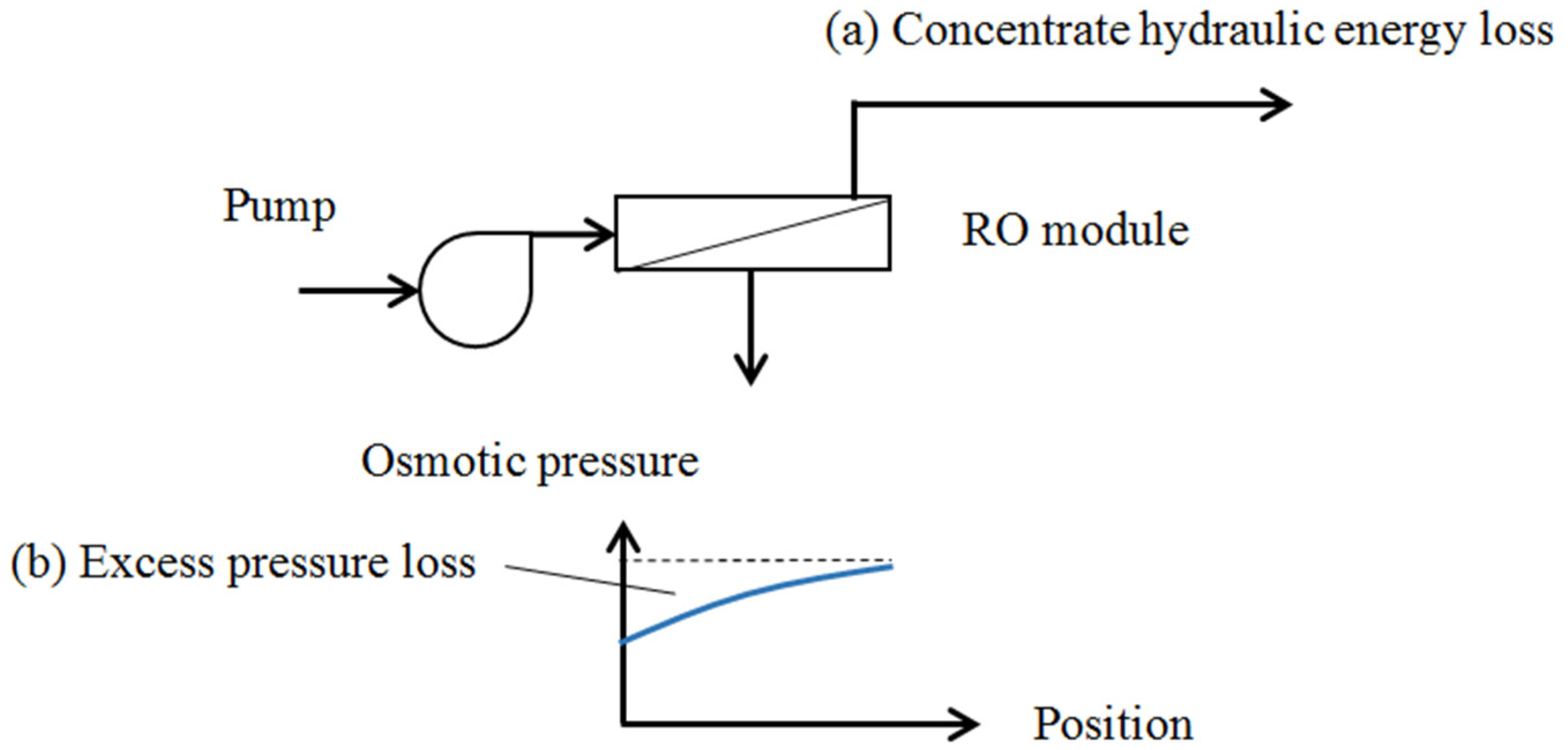
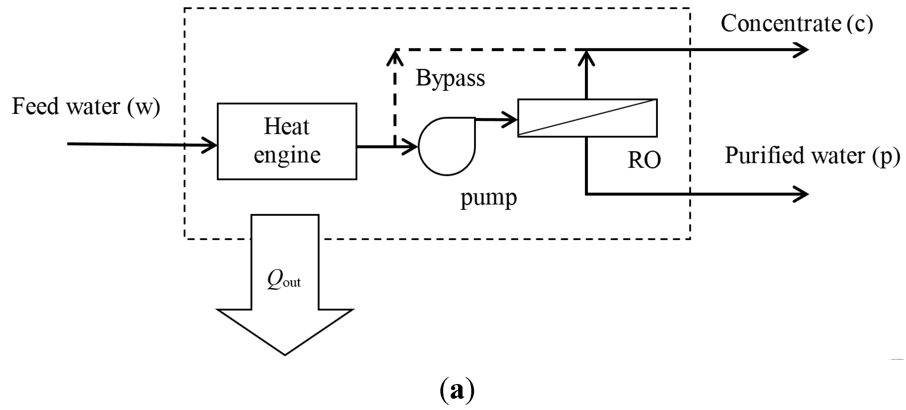
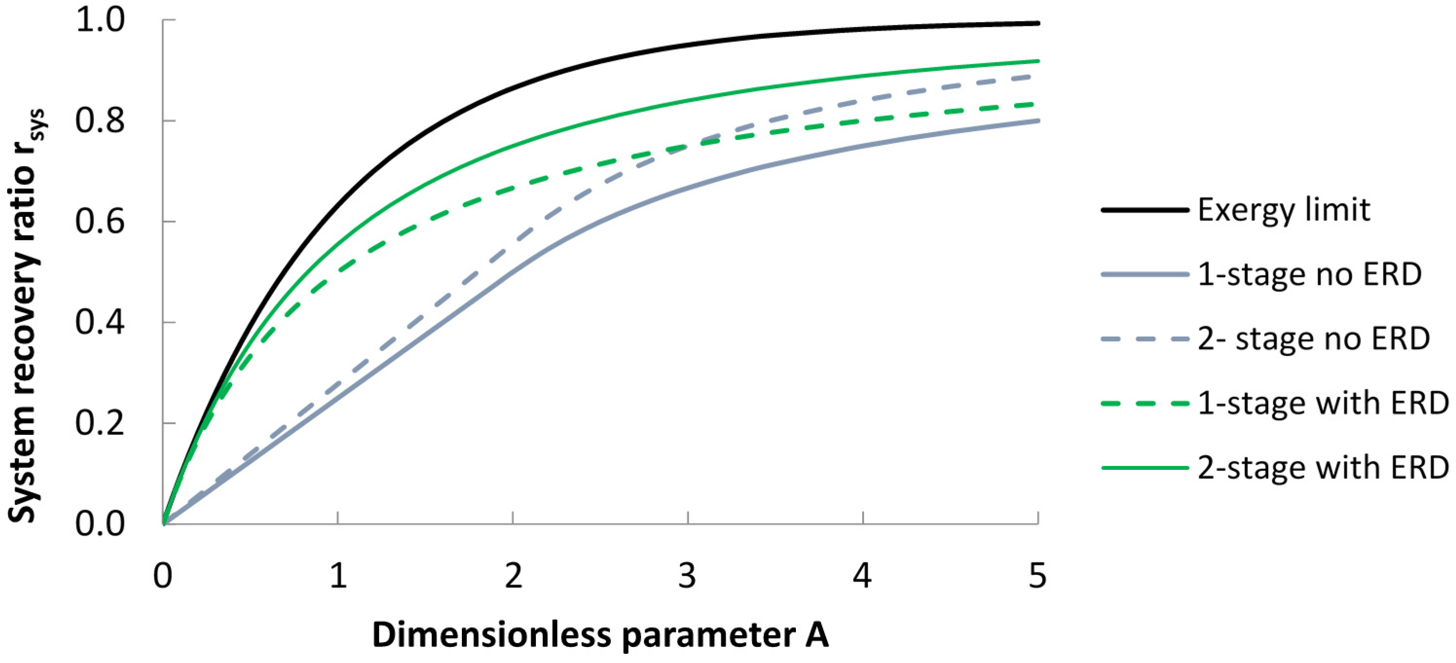
2.2. Reverse Osmosis System

The analysis will now consider the RO process specifically. Rather than assuming a thermodynamically ideal RO process, we will consider semi-ideal RO processes having certain essential losses inherent to the configuration of the system. As defined in this paper, these essential losses are: (a) the loss associated with the hydraulic energy of the concentrate leaving the system; (b) the loss associated with the excess pressure corresponding to the increase in osmotic pressure at the concentrate outlet relative to that at the feed inlet (Figure 2).
Figure 2. Essential losses in a simple Reverse Osmosis (RO) system with no Energy Recovery Device (ERD). Allowing for these losses only, a semi-ideal specific energy consumption SECsideal is defined for the process.
Water 06 03409 g002
The first loss can be eliminated by employing an Energy Recovery Device (ERD); the second can be reduced (but not eliminated) by using multiple stages and intermediate booster pumps [24]. In other words, essential losses cannot be removed without modifying the configuration of the system. In contrast, non-essential losses could in principle be reduced by using higher quality components, by changing the size of components, or by improvements to membrane materials. Non-essential losses include friction losses occurring in the pump or in the pores of the RO membrane.
Because of the essential losses, a RO system having a continuous flow and a finite number of stages always requires more work than specified by Equation (6). For a single stage device without ERD, the osmotic pressure at the outlet is (following the Van’t Hoff expression) increased by a factor of 1/(1 − r) and the minimum work corresponding to Equation (6) becomes:
W s   =   P o s m V w 1 1 r
As Vw is the volume of feed water, the above must be divided by r to get the specific work per volume of purified water i.e., the specific energy consumption:
SEC s i d e a l   =   W s V p   =   P o s m 1 r ( 1 r )
This specific energy consumption is referred to as semi-ideal SECsideal as it takes only essential losses into account. It is greater than SECideal as given by Equation (5). Differentiation of Equation (11) shows that the minimum SECsideal = 2Posm occurs at r = 0.5. For those cases where multiple stages or ERD have been used, formulae for SECsideal given by Qiu and Davies (Table 3 of reference [23]) have been used.
For the case of the single-stage device without ERD, use of Equation (10) in place of Equation (6) leads to a new expression for rsys to be used instead of Equation (11):
r s y s   =   1 1 A
According to the value of A, it may be better to bypass some of the geothermal water around the RO system in which case rsys < r (Figure 3a). This situation occurs when no ERD is used and the value of A is low (A < 2) such that not enough work is available to operate the RO at optimal r = 0.5 while treating the whole feed stream. With the bypass arrangement, the water output is constrained by the work available with the RO system working at r = 0.5 and:
r s y s   =   A 4
Figure 3. Self-powered desalination system comprising a heat engine coupled to a RO system: (a) without energy recovery device with optional bypass of feed water around the RO stage to allow it to work at optimum recovery r = 0.5 for cases where work output from the heat engine is limiting; (b) with energy recovery device (ERD) in which case no such bypass is used.
Water 06 03409 g003aWater 06 03409 g003b
If, on the other hand, there is an excess of work available from the heat engine (A > 2), it is better to avoid the bypass and utilise all this work for maximum water output and thus maximum system recovery rsys even though the stage is then operating sub-optimally at r > 0.5. In this case, Equation (12) applies.
Similar reasoning can be applied to multistage operations to determine whether or not a bypass should be used for cases of no ERD. With the ERD, a low recovery ratio in the RO always results in theoretically lower specific energy consumption; therefore the bypass is never required (Figure 3b).
Expressions analogous to Equation (8) for maximum achievable system recovery rsys, are given in Table 1 for 1- and 2-stage systems with and without energy recovery and these relations are also illustrated in Figure 4 for comparison with the ideal case of Equation (8). Even for the worst case of a stage with no ERD, the prediction is still very promising: A = 2.3 now gives rsys = 0.57. Note however that the heat engine is still assumed to be thermodynamically ideal and non-essential losses of the RO system have not yet been taken into account.
Table 1. Expressions for upper limit to system recovery ratio rsys according to RO configuration, as a function of dimensionless parameter A defined by Equation (9), based on semi-ideal theoretical SECsideal taking into account only essential losses. With a batch system, (or infinitely many stages) the ideal case Equation (8) is reached. In all cases, the system is assumed driven by a reversible heat engine with work output given by Equation (3).
ConfigurationWithout Energy Recovery DeviceWith Energy Recovery Device
1-stageWhen A < 2 (bypass): r s y s = A 1 + A
r s y s = A 4
When A ≥ 2 (no bypass):
r s y s = 1 1 A
2-stageWhen A < 2 (bypass): r s y s = 1 4 ( 2 + A ) 2
rsys = 0.278 A
When A ≥ 2 (no bypass):
r s y s = 1 4 ( 1 + A ) 2
Ideal (batch system, or infinite number of stages with ERD).rsys = 1 − eA
Figure 4. Maximum possible values of system recovery ratio rsys using a reversible geothermal heat engine to drive the desalination process, based on Table 1. Exergy limit is for an ideal reversible RO system (Equation (8)). Lower curves are for theoretical 1- and 2-stage RO systems with and without energy recovery device (ERD), with only essential losses taken into account. Parameter A is defined by Equation (9) (or by Equation (15) once real losses are taken into account).
Water 06 03409 g004
The SEC of real brackish water RO systems is much higher than that given by Equation (11), and the analogous expressions in Table 3 of reference [23], for multistage systems. This is because of several frictional and other non-essential losses including: electrical losses in pump motor, hydraulic losses in pump, frictional losses in pipes, concentration polarization, pore friction loss etc. It is therefore important to compare the theoretical specific energy consumption against real reported systems to obtain a loss ratio εRO which can be used to estimate SEC in proposed systems:
ε R O   =   SEC s i d e a l SEC r e a l
This comparison has been carried out on the basis of systems reported in the literature to reveal values of εRO in the range 0.07–0.14 (Table 2). In this study, a value of εRO = 0.1 is adopted, based on the work of Li and Noh [25], as this is considered a thorough and recent experimental study of a large operational plant. This value, which also concurs with that from the large element study [26], is considered representative of current design and operational practice. Incorporation of this ratio in Equation (14), and use of a similar factor for the ORC system leads to a new expression for the real value of A taking into account all losses.
A r e a l   =   ε R O ψ O R C A
where ψORC is the exergy efficiency of the ORC to be discussed next. The value of Areal thus calculated is then used in place of A in the equations of Table 1 to work out realistic values of achievable rsys.
Table 2. Comparison of theoretical and real specific energy consumptions of some reported brackish water RO systems.
LocationConfiguration *Feedwater ConcentrationOsmotic Pressure PosmRecovery rReported SECrealSemi-Ideal SECsidealLoss Ratio εROCapacityYear ReportedReference
mg kg−1kPakWh m−3kWh m−3m3/day
Kerkennah, Tunisia1-stage no ERD3,700293 **0.751.10.1500.144,7002003[28]
Chino, California (train A)1-stage no ERD950620.8090.4900.03530.078,3002011[29]
Chino, California (train A—optimised)1-stage no ERD950620.90.4410.0440.108,3002012[25]
Large Element Study §1-stage no ERD2,2001750.750.880.0900.10189,0002004[26,30]
Notes: * multiple stages without interstage pump are counted as 1 stage; ** based on assumed NaCl composition; § a detailed design study carried out by consortium of US companies.

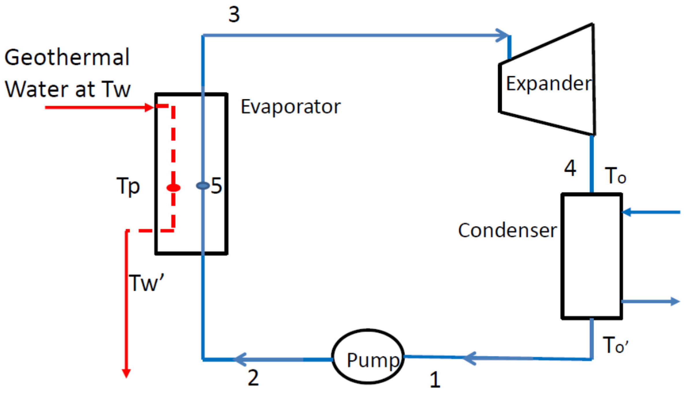
2.3. Organic Rankine Cycle

The calculation of performance for the ORC is based on analysis of thermodynamic cycles using available working fluids. Consistently with Equations (3) and (15), exergy efficiency ψORC is defined by:
ψ O R C   =   p r e d i c t e d   w o r k   o u t p u t   f r o m   O R C e x e r g y   a v a i l a b l e   i n   g e o t h e r m a l   f l u i d
i.e.,
ψ O R C   =   r e a l   w o r k   o u t p u t   f r o m   O R C m ˙ w c p [ ( T w T 0 ) T 0 ln ( T w T 0 ) ]
Note that is the same definition as already used by other authors [13,27].
The properties of the working fluids play a vital role in the cycle performance. Chen et al. [31] reviewed the organic and supercritical Rankine cycles for the conversion of low grade heat into electricity. Several selection criteria of the working fluids were presented and discussed. The type of the working fluids can be dry, wet or isentropic. In total, 35 working fluids were screened and their influence on the performance of the two cycles was analysed. The authors reported that two main criteria—namely the critical temperature and the type of the fluid (dry, wet or isentropic)—are important parameters in indicating the type of cycle a fluid may serve and its operating temperatures [31].
The Rankine cycle analysis is well known and widely used to produce power most commonly using steam as the working fluid. The main components for a basic cycle are the evaporator, turbine, a condenser and a pump. A schematic diagram corresponding to such a basic Rankine cycle is shown in Figure 5.
Figure 5. Schematic of a basic Rankine cycle.
Water 06 03409 g005
An important consideration for the geothermal application is the pinch temperature, defined as (Figure 6):
ΔTp = Tp − T5
Thus, ΔTp = 0 when the temperature profile of the geothermal source intercepts the organic working fluid temperature profile on the saturation curve at the pinch point (5). The energy efficiency of the heat exchanger (evaporator) transferring the geothermal heat to the Rankine cycle working fluid is given by:
η H X   =   T w T w T w T 0
where Tw and Tw refer to the geothermal water temperature entering and leaving the heat exchanger. Similarly, the condenser efficiency can be defined as follows:
η c o n d   =   T 1 T 0 Δ T 0 T 1 T 0
ΔT0 refers to the terminal temperature difference of the condenser defined as the difference between the saturation temperature of the refrigerant and the exit temperature of the coolant.
Figure 6. Temperature profiles of the heat source and the refrigerant in the evaporator.
Water 06 03409 g006
The selection of the most suitable working fluid for this application depends on several factors including the cycle critical temperature, critical pressure and the latent heat. Some other factors and criteria are as summarised in different sources [17,31,32]. These include:
-
Dry expansion to avoid wet vapour and erosion in the turbine;
-
Non-corrosive, non-flammable and non-toxic fluid;
-
High molecular weight to reduce the turbine nozzle velocity;
-
Low ozone depletion potential (ODP) and global warming potential (GWP).
The critical temperature and pressure values of some organic fluids that can be used for low temperature sources are given in Table 3. R143a has the lowest latent heat of evaporation compared to the other refrigerants. This might result in an increase of the required mass flow rate of the organic fluid. Therefore, the size and capacity of the involved equipment would be larger. On the other side, its critical pressure is the lowest; therefore less careful sealing is required to avoid leakage.
Table 3. Some properties of the working fluids considered in this study.
FluidASHRAE DesignationMol. Weight (kg/kmol)Critical Temperature Tc (°C)Critical Pressure Pc (MPa)Latent Heat (at 25 °C) (kJ/kg)ODPGWP
[33][34][34][34][34][35][35]
1,1,1-trifluoroethaneR143a84.0472.73.76159.304470
difluoromethaneR3252.0278.15.78270.90500
propaneR29044.1096.74.25335.303.3
1,1,1,2-tetrafluoroethaneR134a102.03101.04.06177.801430
AmmoniaR71717.03132.311.33116600
In the following, some calculations of the exergy efficiency as defined by Equation (16) are presented for the subcritical ORC. It is of interest to mention that a large number of simulations can be performed for different combinations of the operating variables and conditions governing the ORC system. For instance, the performance of the ORC system and the net power output depend on various parameters including the evaporator pressure, the degree of superheating, the condenser pressure, the turbine and pump isentropic efficiencies as well as the geothermal source temperature profile, the pinch temperature, the condenser terminal temperature difference and the ambient temperature. Therefore and for sake of simplifications, we choose in the following section to fix several parameters as follows:
Expander isentropic efficiency = 0.85, pump isentropic efficiency = 0.9, condenser terminal temperature difference ΔT0 = 2 °C, pinch temperature difference ΔTp = 2 °C. T3 (refrigerant temperature at the expander inlet) = Twin − 2ΔTp.
In the above calculations, Engineering Equation Solver (EES) [34] was used to evaluate ψORC. The basic equations for the cycle are well known and can be found in many sources e.g., [36]. They were obtained using steady state energy and mass balances for each component of the system as well as for the whole ORC unit. An optimisation method based on the quadratic approximation one was applied to maximise ψORC by changing the evaporation pressure and the condensation pressure subsequently. The objective function to maximise here was the exergy efficiency ψORC.

3. Case Studies

3.1. Case Study 1: Tuwa, Gujarat

The north-western Indian state of Gujarat is a relatively dry area of the Indian sub-continent. Rainfall averages about 800 mm per year, but is confined mainly to the monsoon season, and shows considerable year-to-year variation in timing and intensity [37]. Much of soils and groundwater in Gujarat is affected by salts [38]. Rapid expansion of the population and economy in India in recent years has led to energy shortages and frequent electricity power outages. Therefore, it is highly desirable that new water treatment methods should be independent of the electricity grid, especially in remote areas.
Interestingly, several thermal springs have been identified in Gujarat and neighbouring Rajasthan. According to Minnesale et al. [39], springs in Rajasthan emerge at 50 °C or below, whereas those in Gujarat emerge at up to 93 °C. Therefore the Rajasthan springs are considered too cool to power the ORC. This study focusses instead on the Gujarat sources located in the Tuwa area, about 60 km east of Ahmadabad. The temperatures of these springs range from 41 to 93 °C and salinities from 2838 to 5973 mg kg−1 (Figure 7).
It was observed that the spring with temperature of 60 °C and salinity of 3351 mg kg−1 (Tuwa 5) was the most representative. Therefore this spring is used as the basis for the case study. The composition of electrolytes in Tuwa 5 is predominantly sodium chloride, with calcium and sulphate ions also present (Figure 8a). Tuwa 5 water also contains a high level of silica (122 mg kg−1). This relative composition is also representative of the other springs at Tuwa.
The ambient temperature T0 for this case study was chosen as the average daily maximum of 41 °C for the hottest month of May, as the greatest water demand is likely to occur at the hottest time of year. Based on the Van’t Hoff law and using the osmotic coefficients as in the Appendix, the osmotic pressure of the solution was calculated to be 245 kPa for Tuwa 5 at this temperature.
Figure 7. Temperatures and salinities of the thermal springs in the Tuwa area of Gujarat [39].
Water 06 03409 g007

3.2. Case Study 2: Salbukh, Najd Plateau, Saudi Arabia

Like other Gulf Cooperation Countries, Saudi Arabia is experiencing simultaneous growth in population, energy demand and water demand [40]. The central Najd Plateau accommodates several cities including Riyadh which currently has a population of 5 million, increased from 3.5 million in 2000. With typically less than 20 mm of rain per year, these cities are heavily reliant on piped desalinated water or on exploitation of aquifers which are generally saline. The elevation of the Najd Plateau is some 762–1525 m above sea level and, with inland areas located some 700 km from the coastline, the energy cost of desalinating seawater and pumping it to inland cities exceeds 7 kWh m−3 [41]. This gives a strong incentive to make use of inland water sources but such use requires desalination at high recovery to avoid problems of pollution by the concentrate.
Sobhani et al. [41] sampled 10 inland aquifers of Saudi Arabia and reported salinities in the range 386–2914 mg kg−1. The samples were rich in sodium, calcium, magnesium, chloride and sulphate, as shown by the example composition of Figure 8b. Many groundwater sources show geothermal activity. In the Riyadh area, the wells at Salbukh and Albobb are reported to emerge at 70 °C. Salbukh is taken as the case for use in this study. The well water has salinity of 1800 mg kg−1 which, based on the same relative composition as in Figure 8b, gives an osmotic pressure of 117 kPa.
Figure 8. Compositions of groundwater corresponding to case studies (a) Tuwa 5 spring in Gujarat, India [39]; (b) Site A on Najd Plateau, Saudi Arabia [41]; (c) intercalaire aquifer near Kebili, Tunisia [42]; (d) Eynal Spring, Turkey (reported in [45]).
Water 06 03409 g008

3.3. Case Study 3: Kebili Geothermal Field, Tunisia

The Kebili geothermal field lies above the intercalaire aquifer which covers an area of 600,000 km2 extending into Tunisia, Algeria and Libya [42]. This large aquifer is already exploited in Tunisia for the heating of greenhouses, bathing, and for irrigation of crops. However, the water is reported to have salinities in the range 2500–5000 mg kg−1 and this makes the water unsuitable for human consumption and only marginally suitable for agriculture [43]. Typically the water emerges at 70 °C and it is sometimes passed through cooling towers to dissipate the heat prior to utilization [44].
Agoun [42] has provided analyses of samples from 10 wells from the intercalaire near Kebili with TDS ranging from 1840 to 2870 mg kg−1. Based on these a median value of 2440 mg kg−1 (well number 7) was selected; its chemical analysis shows high sodium, calcium, magnesium, chloride and sulphate (Figure 8c below). The average daily maximum temperature in Kebili is 38 °C in July–August and this was taken as the value of T0.

3.4. Case Study 4: Eynal Spring, Simav Geothermal Field, Turkey

The Simav geothermal field in Kütahaya province of Western Anatolia is one of 170 geothermal fields in Turkey with temperature over 40 °C [45]. Reservoir rock temperatures for this field have been calculated in the range 148–180 °C. The Eynal Spring reportedly emerges at 96 °C and is taken here as a relatively high temperature source at atmospheric temperature, combined with relatively low salinity 1830 mg kg−1. The composition of the Eynal Spring consists mainly of sodium sulphate and sodium bicarbonate and as shown in Figure 8d below. These result in an osmotic pressure of 97 kPa at ambient temperature of 31 °C. The water also contains a significant level of silica (54 mg kg−1).

4. Results

The ideal exergy limit of Equation (8) applied to all four case studies gives rsys > 0.99 (Table 4). Whereas this very high value is not presented as a practically achievable level of system recovery (e.g., because it would lead to problems of membrane scaling) it does indicate the sound theoretical feasibility of achieving self-powered geothermal desalination at good recovery even for very low enthalpy sources at temperatures below 70 °C. Semi-ideal assumptions, with only essential RO losses taken into account, also predict high values of rsys ≥ 0.89 in all cases—even using single stage RO systems with no ERD.
Table 4. Calculated values of system recovery rsys using the organic Rankine cycle and reverse osmosis under ideal, semi-ideal and real assumptions.
Case Study
1. Tuwa—Gujarat (India)2. Salbukh—(Saudi Arabia)3. Kebili—(Tunisia)4. Eynal—(Turkey)
Total salt concentration (mg/kg)3350180024401830
Osmotic Pressure (kPa)24511711997.5
Source temperature T160707096
Ambient temperature T041443831
Parameter A9.436.154.1261.2
ψORC (R290)0.30850.32710.3730.4503
εRO0.100.100.100.10
Areal0.291.182.0211.76
Maximum rsys
Ideal exergetic limit * >0.99>0.99>0.99>0.99
Semi-ideal **:
1-stage RO (no ERD)0.8940.9720.982>0.99
2-stage RO (no ERD)0.963>0.99>0.99>0.99
1-stage RO (with ERD)0.9040.9730.982>0.99
2-stage RO (with ERD)0.969>0.99>0.99>0.99
Real §:
1-stage RO (no ERD)0.0730.2950.5050.915
2-stage RO (no ERD)0.0810.3280.5610.975
1-stage RO (with ERD) 0.2250.5420.6690.922
2-stage RO (with ERD)0.2380.6050.7520.979
Notes: * based on Equations (8) and (9); ** Table 1, based on A; § Table 1, based on Areal.
The thermodynamic cycle calculations yield results for ψORC in the range 0.286–0.450 (Table 5). Of the two refrigerants investigated, propane (R290) gives slightly better performance than R143a for the lower temperature applications, and worse for the higher temperature ones. Because the differences are not large, propane is preferred because of its better environmental properties with respect to global warming and ozone depletion (Table 3).
Table 5. Results for exergy efficiency ψORC as a function of the source and ambient temperatures for two working fluids (R143a and R290).
Case Study
1. Tuwa—Gujarat (India)2. Salbukh—(Saudi Arabia)3. Kebili—(Tunisia)4. Eynal—(Turkey)
Source temperature Tw60707096
Ambient temperature T041443831
R143aψORC0.2860.3590.3660.563
(Pevap, Pcond)(2390,2000)(2756,2115)(2756,1850)(3700,1550)
R290 (propane)ψORC0.30850.32710.3730.4503
(Pevap, Pcond)(1754,1468)(1899,1570)(1899,1370)(2408,1165)
These results for ψORC for propane, together with the practically observed values of εRO for real RO plant, give values of rsys in the range 0.073−0.979. These are much lower than the values based on ideal and semi-ideal assumptions. The difference is most significant for Tuwa (case study 1, geothermal water supplied at only 60 °C) where using single-stage RO without ERD, only rsys = 0.073 is predicted which would be unsatisfactory as effectively 93% of the source water would be wasted. Use of ERD improves this significantly to rsys = 0.225. On the other hand, for the Eynal Spring emerging at 96 °C (case study 4), rsys has a high value of 0.915 even for a single-stage system without ERD.
The results therefore emphasize the critical effect of the geothermal source temperature in determining the technical feasibility of the self-powered desalination. For case study 1, though it is feasible under ideal assumptions, under more realistic assumptions it becomes only marginally feasible. The main reason is the substantial gap between the SEC of actual brackish water plant and the thermodynamic minimum, as represented by the low loss ratio εRO = 0.1. This occurs because brackish water RO plants typically operate at well above the osmotic pressure [29]. In comparison, seawater desalination plants have lower values of εRO; for example, at 3.5 kWh/m3 εRO = 0.2. Using this value of εRO in the current calculations would give, for case study 1, a value of rsys increased from 0.225 to 0.368 (single-stage, with ERD).

5. Discussion

5.1. Pre- and Post-Treatment

The exergy analysis has not considered pre- or post-treatment. Based on the water compositions of the case studies, some preliminary observations about these additional process and likely energy requirements are now made. Both physical and chemical pre-treatments may be required.
All cases would likely require removal of insoluble foulants in the form of particles and colloids. This may be achieved through conventional or membrane pre-treatment. Conventional pre-treatment typically includes several steps such as flocculation, sand filtration and cartridge filtration. Membrane pre-treatment, comprising ultrafiltration (UF) or microfiltration (MF), is being increasingly adopted as it is more modular and compact than conventional pre-treatment. It also requires smaller amounts of chemicals. Nonetheless, these membrane filters have to be periodically cleaned by back-flushing [46].
In a mobile desalination system for brackish water sources, Schäfer et al. [47] used UF pre-treatment to protect RO membranes against fouling. They found that the UF membranes introduced a pressure differential of 0.5 bar, compared to 12 bar across the RO membranes. This suggests that the energy requirement for the UF pre-treatment is an order of magnitude lower than for the RO treatment. Nonetheless, their design used six UF modules to precede one RO module—suggesting that UF pre-treatment adds significantly to the overall capital cost.
Chemical pre-treatment is important to avoid biological growth and avoid scaling. Water from deep boreholes is not expected to contain high biological activity. However, due to its prolonged contact with minerals, levels of calcium, magnesium, sulphate, (bi)carbonates and silica may be high. These species are prone to form insoluble scale on the membrane surface which will decrease flux and increase energy requirement. The likelihood of scaling may be assessed through solubility product calculations and increases with increasing recovery ratio [46]. In all four case studies, calcium and carbonates are present at significant levels such that it will be important to dose with hydrochloric acid to maintain low pH which favours formation of relatively soluble bicarbonate ions. The compositions of the four case studies suggest additional chemical pre-treatments such as anti-scalants will be needed, as shown in Table 6.
Table 6. Scaling and preventative chemical pre-treatments for the four case studies.
Case StudyScaling IssuePre-Treatment
1: Tuwa, GujaratCalcium sulphate precipitation would limit recovery to about 0.3High silica levelUse anti-scalants e.g., phosphonates (or work at lower recovery)
2: Salbukh, Saudi ArabiaCalcium sulphate already near saturationAnti-scalant or water softening by cation-exchange resin
3: Kebili, Tunisia
4: Eynal Spring, TurkeyCalcium sulphate precipitation would limit recovery to about 0.5Significant silica levelUse anti-scalants e.g., phosphonates (or work at lower recovery)
Post-treatment can include remineralisation and disinfection processes [46]. Such processes generally require little energy compared to the RO operation but they would contribute to the overall plant cost.

5.2. Equipment Design for Performance and Low Cost

The results show that, though self-powered desalination is possible in principle, great care is needed in the design of the plant to minimise losses. This will require correct design choices at both the conceptual and detailed level. To minimise the essential losses, a batch RO system would be preferable to a multi-stage continuous flow design. The batch system does not require a separate ERD and is equivalent in performance to an infinite number of stages, even though it may contain only one RO module [23,48]. The batch system does, however, require valves in addition to pumps and these should be selected carefully for low cost and reliable operation. To lower the operating pressure, the flux in the RO system should be kept low, so that the system works closer to thermodynamic equilibrium. However, this would require a larger membrane area which would increase the cost. In addition, if the pressure is too low, salt passage through the membrane may become unacceptably high.
The ORC system must also be designed to minimise thermodynamic irreversibilities. Thus, large evaporator and condenser surface areas are needed to achieve the required small temperature differentials (2 °C). This again introduces an economic consideration. A comprehensive design optimisation would require overall cost to be minimised for a given performance, by means of a parametric study. For example, El-Emam and Dincer [13] have carried out such an exercise for a geothermal ORC which could in future be extended to cover the RO within the self-powered desalination concept. Alternative conceptual approaches to enhancing ORC performance could be aimed at overcoming the limitation posed by the pinch point e.g., use of the Kalina cycle, or supercritical cycles to introduce a more nearly linear T-h characteristic in the evaporator. These approaches may be the subject of future studies.

6. Conclusions

This work has demonstrated the feasibility of self-powered desalination of geothermal saline groundwater without input from any external power source. A general method and framework has been developed and then applied to specific case studies of geothermal waters at <100 °C. An exergy approach has been used, with ideal, semi-ideal and realistic assumptions introduced. Desalination performance has been quantified in terms of the overall system recovery ratio rsys.
For the idealized limit, exergy constraints place virtually no limit on performance (rsys > 0.99). Under semi-ideal assumptions, whereby only essential losses in a RO system are taken into account, achievable recovery remains very high (rsys > 0.89) even for single-stage RO without ERD which is the least efficient arrangement.
However, taking into account realistic losses in the RO system and in an ORC driving it, the analysis shows that performance may in practice be considerably lower and depends critically on the source temperature. Thus, for the case of Tuwa, Gujarat (Tw = 60 °C) rsys is in the range 0.073−0.238; while for the Eynal Spring, Turkey (Tw = 96 °C) rsys = 0.915–0.979. These results give considerable incentive to develop, optimise and apply geothermal desalination as a dependable source of fresh water for a number of arid areas. The framework presented here should be developed further to incorporate more detailed engineering and economic data such that these systems can be practically realized.
For geothermal sources above 100 °C, the study has shown that the ORC can provide more than enough work for RO desalination. Therefore, future studies should encompass combined systems for both water and power, thus realizing the original vision of Awerbuch et al. [3] while taking advantage of modern RO and ORC technology.

Nomenclature

A
dimensionless parameter defined by Equation (9)
mass flow (kg s−1)
n
moles of solute (kmol)
P
pressure (kPa)
r
recovery ratio
R
gas constant ( = 8.314 kJ·kmol−1·K−1)
T
temperature (K or °C)
V
volume (m3)
V ˙
volumetric flow (m3·s−1)
W
mechanical work (kJ)
rate of mechanical work (kW)
SEC
specific energy consumption (kJ m−3 or kWh m−3)

Greek letters

ε
loss ratio
η
energy efficiency
ψ
exergy efficiency

Subscripts

c
concentrate
cond
condenser
evap
evaporator
ideal
ideal
p
purified water (permeate), or pinch point
ORC
organic Rankine cycle
osm
osmotic
real
real
RO
reverse osmosis
s
relating to work of desalination
sideal
semi-ideal
sys
system
t
relating to conversion of thermal energy to work
w
feedwater at system inlet
w’
feedwater at outlet to heat exchanger
0
ambient
0’
at condenser outlet
1
at pump inlet
2
at pump outlet
3
at evaporator outlet
4
at expander outlet
5
pinch point

Abbreviations

ERD
Energy Recovery Device
GWP
Global Warming Potential
MSF
Multi-stage Flash Unit
ODP
Ozone Depleting Potential
ORC
Organic Rankine Cycle
RO
Reverse Osmosis

Acknowledgments

Philip A. Davies acknowledges support from the King Saud University Visiting Professor Program. Jamel Orfi acknowledges support from the Aston University Visiting Scholars’ Fund.

Author Contributions

Philip A. Davies defined the initial framework for the study and performed the analysis of the RO systems. Jamel Orfi carried out the ORC cycle analysis. Both authors contributed to the interpretation of results.

Appendix: Calculation of Osmotic Pressures

Calculations of the energy requirement for desalination by RO require the osmotic pressure to be known. Because only brackish water sources of low concentration are considered here, the calculation of the osmotic pressure P is based on the classical Van’t Hoff expression:
P   =   R T i υ i α i n i V
where ni/V is the molar concentration (kmol/m3) of each species present; vi the number of ions available by complete dissociation each species (e.g., 2 for NaCl, 3 for CaCl2); and ai is the osmotic coefficient for each species, which is generally close to unity. Table A1 gives the osmotic coefficients used in this study for dilute solutions of the main salts occurring in the sources considered. Based on the data in [49], this approach was found to give good representation of osmotic pressure up to concentrations of 0.4 kmol m−3, which is an order of magnitude higher than encountered in this study. It was also found to predict the osmotic pressure of diluted seawater (concentration 18,039 mg/kg) with less than 1% error [50]. Therefore Equation (A1) is considered to be of good accuracy and is preferred over more complex methods of calculating the osmotic pressure, because it is a linear equation which greatly simplifies the analysis.
Table A1. Osmotic coefficients for dilute solutions used in Equation (A1).
SaltOsmotic Coefficient aSource
NaCl0.932[49] at 0.1 mol kg−1
CaCl20.854
MgCl20.861
Na2SO40.793
NaHCO30.909[51]

Conflicts of Interest

The authors declare no conflict of interest.

References

  1. Lund, J.W.; Freeston, D.H.; Boyd, T.L. Direct utilization of geothermal energy in 2010 worldwide. Geothermics 2011, 40, 159–180. [Google Scholar] [CrossRef]
  2. Dincer, I.; Hepbasli, A.; Ozgener, L. Geothermal energy resources. In Encyclopedia of Energy Engineering and Technology; CRC Press (Taylor and Francis Group): Boca Raton, FL, USA, 2007; pp. 744–752. [Google Scholar]
  3. Awerbuch, L.; Lindemuth, T.E.; May, S.C.; Rogers, A.N. Geothermal energy recovery process. Desalination 1976, 9, 325–336. [Google Scholar] [CrossRef]
  4. Bourouni, K.; Chaibi, M.; Martin, R.; Tadrist, L. Heat Transfer and evaporation in geothermal desalination units. Appl. Energy 1999, 64, 129–147. [Google Scholar] [CrossRef]
  5. Mohamed, A.M.I.; El Minshawy, N.A.S. Humidification-dehumidification desalination system driven by geothermal energy. Desalination 2009, 249, 602–608. [Google Scholar] [CrossRef]
  6. Mahmoudi, H.; Spahis, N.; Goosen, M.F.; Ghaffour, N.; Drouiche, N.; Ouagued, A. Application of geothermal energy for heating and fresh water production in a brackish water greenhouse desalination unit: A case study from Algeria. Renew. Sust. Energy Rev. 2010, 14, 512–517. [Google Scholar] [CrossRef]
  7. Bouguecha, S.; Dhahb, M. Fluidised bed crystalliser and air gap membrane distillation as a solution to geothermal water desalination. Desalination 2003, 152, 237–244. [Google Scholar] [CrossRef]
  8. Mathioulakis, E.; Belessiotis, V.; Delyannis, E. Desalination by using alternative energy: Review and state-of-the-art. Desalination 2007, 152, 346–365. [Google Scholar] [CrossRef]
  9. Koroneos, C.; Roumbas, G. Geothermal waters heat integration for the desalination of sea water. Desalin. Water Treat. 2012, 37, 69–76. [Google Scholar] [CrossRef]
  10. Li, C.; Besarati, S.; Goswami, Y.; Stefanokos, E.; Chen, H. Reverse osmosis desalination driven by low temperature supercritical organic Rankine cycle. Appl. Energy 2013, 102, 1071–1080. [Google Scholar] [CrossRef]
  11. Manolakos, D.; Papadakis, G.; Kyritsis, S.; Bouzianas, K. Experimental evaluation of an autonomous low-temperature solar Rankine cycle system for reverse osmosis desalination. Desalination 2007, 203, 366–374. [Google Scholar] [CrossRef]
  12. Igobo, O.N.; Davies, P.A. Low-temperature organic Rankine cycle engine with isothermal expansion for use in desalination. Desalin. Water Treat. 2014. [Google Scholar] [CrossRef]
  13. El-Emam, R.S.; Dincer, I. Exergy and exergoecomomic analyses and optimization of geothermal Rankine cycle. Appl. Therm. Eng. 2013, 59, 435–444. [Google Scholar] [CrossRef]
  14. Madhawa Hettiarachchi, H.D.; Golubovic, M.; Worek, W.M.; Ikegami, Y. Optimum design criteria for an Organic Rankine cycle using low-temperature geothermal heat sources. Energy 2007, 32, 1698–1706. [Google Scholar] [CrossRef]
  15. Cerci, Y. Exergy analysis of a reverse osmosis desalination plant in California. Desalination 2002, 142, 257–266. [Google Scholar] [CrossRef]
  16. El-Emam, R.S.; Dincer, I. Thermodynamic and thermoeconomic analyses of seawater reverse osmosis desalination plant with energy recovery. Energy 2014, 64, 154–163. [Google Scholar] [CrossRef]
  17. Nafey, A.S.; Sharaf, M.A. Combined solar organic Rankine cycle with reverse osmosis desalination process: Energy, exergy and cost evaluations. Renew. Energy 2010, 35, 2571–2580. [Google Scholar] [CrossRef]
  18. Tchanche, B.F.; Lambrinos, G.; Frangoudakis, A.; Papadakis, G. Exergy analysis of micro-organic Rankine power cycles for a small scale solar driven reverse osmosis desalination system. Appl. Energy 2010, 87, 1295–1306. [Google Scholar] [CrossRef]
  19. Bejan, A. Advanced Engineering Thermodynamics; Wiley: New York, NY, USA, 1988. [Google Scholar]
  20. Feistel, R. A Gibbs function for seawater thermodynamics for −6 to 80 °C and salinity up to 120 g kg−1. Deep Sea Res. I 2008, 55, 1639–1671. [Google Scholar]
  21. Mistry, K.H.; Hunter, H.A.; Lienhard, J.H. Effect of composition and nonideal solution behavior on desalination calculations for mixed electrolyte solutions with comparison to seawater. Desalination 2013, 318, 34–47. [Google Scholar] [CrossRef]
  22. Sharqawy, M.H.; Lienhard, J.H.; Zubair, S.M. Thermophysical properties of seawater: A review of existing correlations and data. Desalin. Water Treat. 2010, 16, 354–380. [Google Scholar] [CrossRef]
  23. Qiu, T.; Davies, P.A. Comparison of configurations for high-recovery inland desalination systems. Water 2012, 4, 690–706. [Google Scholar] [CrossRef]
  24. Elimelech, M.; Phillip, W.A. The future of seawater desalination: Energy, technology and the environment. Science 2011, 333, 712–717. [Google Scholar] [CrossRef] [PubMed]
  25. Li, M.; Noh, B. Validation of model-based validation of brackish water reverse osmosis (BWRO) desalination. Desalination 2012, 304, 20–24. [Google Scholar] [CrossRef]
  26. Bartels, C.; Bergman, R.; Hallan, M.; Henthorne, L.; Knappe, P.; Lozier, J.; Metcalfe, P.; Peery, M.; Shelby, I. Industry Consortium Analysis of Large Reverse Osmosis and Nanofiltration Element Diameters; Desalination and Water Purification Research and Development Report No. 114; US Bureau of Reclamation: Denver, CO, USA, 2004. [Google Scholar]
  27. He, C.; Liu, C.; Gao, H.; Li, Y.; Wu, S.; Xu, J. The optimal evaporation temperature and working fluids for subcritical organic Rankine cycle. Energy 2012, 38, 136–143. [Google Scholar] [CrossRef]
  28. Fethi, K. Optimization of energy consumption in the 3300 m3/d RO Kerkennah plant. Desalination 2003, 157, 145–149. [Google Scholar] [CrossRef]
  29. Li, M. Optimal plant operation of brackish water reverse osmosis (BWRO) desalination. Desalination 2012, 239, 61–68. [Google Scholar] [CrossRef]
  30. Pearce, G.K. UF/MF pre-treatment to RO in seawater and wastewater reuse applications: A comparison of energy costs. Desalination 2008, 222, 66–73. [Google Scholar] [CrossRef]
  31. Chen, H.; Goswami, D.Y.; Stefanokos, E.K. A review of thermoadynamic cycles and working fluids for the conversion of low grade heat. Renew. Sust. Energy Rev. 2010, 14, 3059–3067. [Google Scholar] [CrossRef]
  32. Nguyen, T.Q.; Slawnwhite, J.D.; Goni Boulama, K. Power generation from residual industrial heat. Energy Conv. Manag. 2010, 51, 2220–2229. [Google Scholar] [CrossRef]
  33. Doerr, R.G. Refrigerants; ASHRAE Handbook: Atlanta, GA, USA, 2001; Chapter 19. [Google Scholar]
  34. Klein, S.A. Engineering Equation Solver (EES); F-Chart Software: Madison, WI, USA, 2013. [Google Scholar]
  35. Environment Canada, Govt. of Canada. Available online: http://www.ec.gc.ca/Air/ (accessed on 15 October 2014).
  36. Khennich, M.; Galanis, N. Thermodynamic analysis and optimization of power cycles sing a finite low temperature heat source. Int. J. Energy Res. 2012, 36, 871–885. [Google Scholar] [CrossRef]
  37. World Meteorological Organisation (WMO). Available online: http://www.wmo.int (accessed on 16 Janurary 2014).
  38. Singh, G. Salinity-related desertification and management strategies: Indian experience. Land Degrad. Dev. 2009, 20, 367–385. [Google Scholar] [CrossRef]
  39. Minissale, A.; Chandrasekharam, D.; Vaselli, O.; Magro, G.; Tassi, F.; Pansini, G.L.; Bhramhabut, A. Geochemistry, geothermics and relationship to active tectonics of Gujarat and Rajasthan thermal discharges, India. J. Volcanol. Geotherm. Res. 2003, 127, 19–32. [Google Scholar] [CrossRef]
  40. Electricity and Cogeneration Regulatory Authority (ECRA). Annual Statistical Booklet and Seawater Desalination Industries; ECRA: Riyadh, Saudi Arabia, 2012. [Google Scholar]
  41. Sobhani, R.; Abahusayn, M.; Gabelich, C.J.; Rosso, D. Energy footprint analysis of brackish groundwater desalination with zero liquid discharge in inland areas of the Arabian Peninsula. Desalination 2012, 291, 106–116. [Google Scholar] [CrossRef]
  42. Agoun, A. Exploitation of the Continental Intercalaire Aquifer at the Kebili Geothermal Field, Tunisia; Report No 2; UN University Geothermal Training Programme: Reykjavík, Iceland, 2000. [Google Scholar]
  43. Bourouni, K.; Chaibi, M.T. Application of geothermal energy for brackish water desalination in South of Tunisia. In Proceedings of World Geothermal Congress, Antalya, Turkey, 24–29 April 2005.
  44. Bourouni, K.; Chaibi, M.T. Geothermal water cooling systems in Tunisia—Design and practice. In Proceedings of World Geothermal Congress, Antalya, Turkey, 24–29 April 2005.
  45. Bayram, A.F.; Simsek, S. Hydrogeochemical isotopic survey of Kütahya-Simav geothermal field. In Proceedings of World Geothermal Congress, Antalya, Turkey, 24–29 April 2005.
  46. Fritzmann, C.; Löwenberg, J.; Wintgens, T.; Melin, T. State-of-the-art reverse osmosis desalination. Desalination 2007, 216, 1–76. [Google Scholar] [CrossRef]
  47. Schäfer, A.; Broeckmann, A.; Richards, B.S. Renewable energy powered membrane technology: 1. Development and characterization of a photovoltaic hybrid membrane system. Environ. Sci. Technol. 2007, 41, 998–1003. [Google Scholar] [CrossRef] [PubMed]
  48. Qiu, T.Y.; Igobo, O.N.; Davies, P.A. DesaLink: Solar-powered desalination of brackish groundwater giving high output and high recovery. Desalin. Water Treat. 2013, 51, 1279–1289. [Google Scholar] [CrossRef]
  49. Robinson, R.A.; Stokes, R.H. Electrolyte Solutions; Butterworths: London, UK, 1959. [Google Scholar]
  50. Robinson, R.A. The vapour pressure and osmotic equivalence of sea water. J. Mar. Biol. Assoc. UK 1954, 33, 449–455. [Google Scholar] [CrossRef]
  51. Sarbar, M.; Convington, A.K.; Nuttall, R.L.; Goldberg, R.N. The activity and osmotic coefficients of aqueous sodium bicarbonate solutions. J. Chem. Thermodyn. 1982, 14, 967–976. [Google Scholar] [CrossRef]

