1. Introduction
The Aral-Caspian basin is the major internal drainage area of Central Asia. Its 4,000,000 km
2 are 75% steppe and desert [
1]. However, large amounts of water are stored in glaciers, permafrost and snow on high mountain ridges in Kyrgyzstan and Tajikistan in the East of Central Asia. At present, these water storages play the key role in the water management that has to regulate the supply for the livelihood in the Central Asian lowlands including main parts of the Ferghana valley in Uzbekistan (
Figure 1, 39.4°–42° N, 69.2°–73.8° E) [
2,
3,
4,
5]. The valley floor at about 400 m is surrounded by the mountain ranges of the Tien Shan and the Alay mountain systems that reach up to 5000 m a.s.l.: the Chatkal ridge in the north, the Ferghana ridge in the east and the Alay ridge in the south. These orographic conditions protect the valley against the invasion of cold air masses from the north but open it to relatively moist air from the west [
3,
6,
7]. Therefore, the Ferghana Valley has relatively warm winters and hot summers [
8]. As the moist air from the west is forced to move upwards, which includes adiabatic cooling, the precipitation generally increases with elevation and reaches up to 1300 mm per year at the northwestern slopes of the Ferghana ridge [
8,
9].
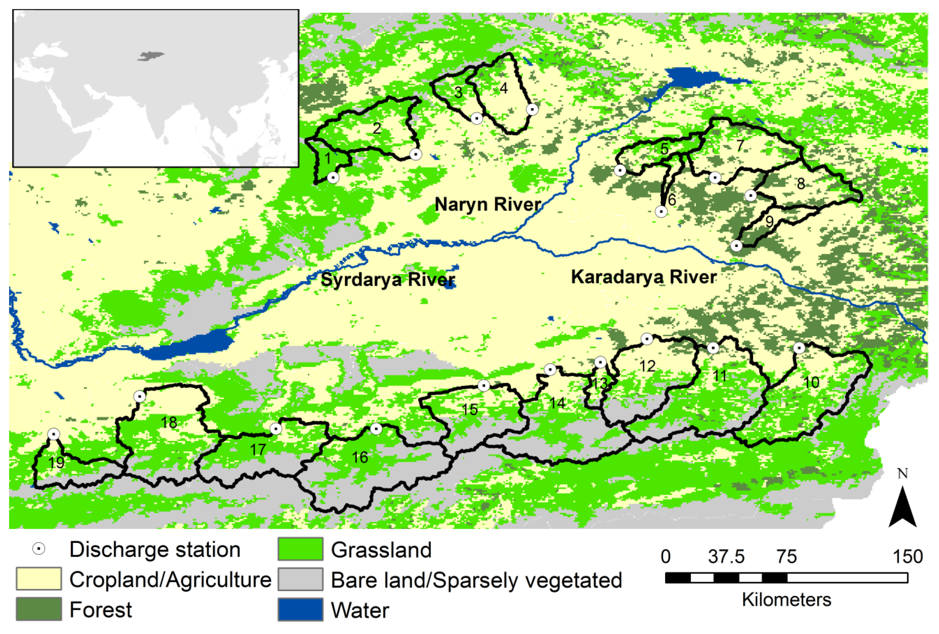
Figure 1.
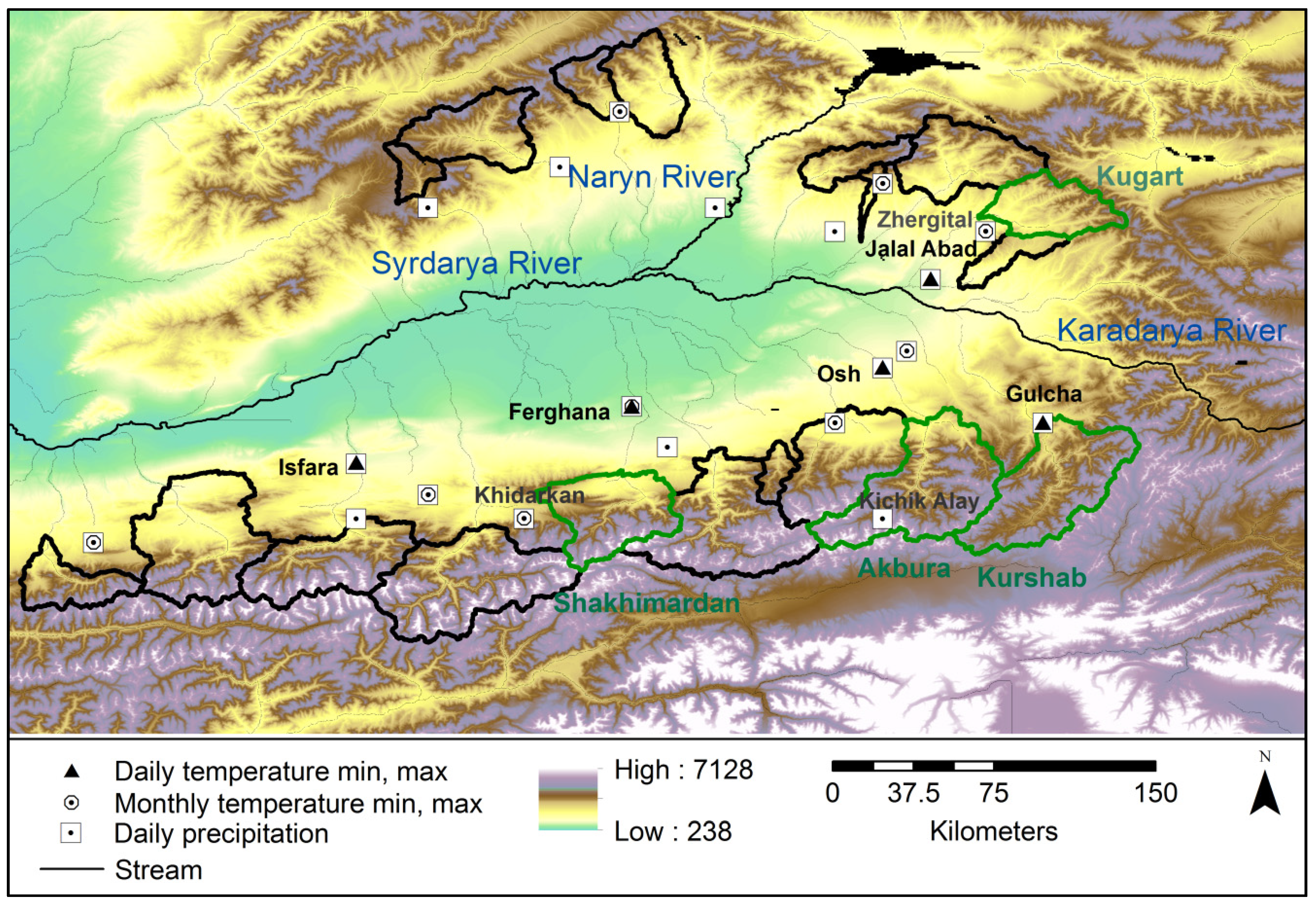
The Ferghana Valley with FAO (Food and Agriculture Organization) land-use map and delineated upper catchments (in black) using SRTM (Shuttle Radar Topography Mission) DEM (Digital Elevation Model, 90 m) and ArcGIS (10) software (Redlands, CA, USA).
Figure 1.
The Ferghana Valley with FAO (Food and Agriculture Organization) land-use map and delineated upper catchments (in black) using SRTM (Shuttle Radar Topography Mission) DEM (Digital Elevation Model, 90 m) and ArcGIS (10) software (Redlands, CA, USA).
The Karadarya and Naryn rivers have their source in the eastern part of the Ferghana Valley and the Tien Shan mountain system in Kyrgyzstan, from where during summer they are mainly fed by glaciers and snow melt. The confluence of the two rivers in the Uzbek part of the Ferghana Valley forms the Syrdarya River. This river is the main water artery of the valley with a mean discharge of about 39 km
3·year
−1 [
10]. Kyrgyzstan and the three countries Tajikistan, Uzbekistan and Kazakhstan contribute 74% and 26% of the water volume of the Syrdarya River, respectively [
1]. Smaller streams and catchments at the proximate northern, eastern and southern ridges around Ferghana Valley contribute water mainly from annual rain and snowfall and only a few streams to the south include some glacial melt.
A data compilation of the contributions of the two main and the most relevant smaller rivers shows that (a) the 19 smaller catchments (individually 71–2480 km
2) cover together an area of around 23,700 km
2 or 36% of the combined headwater areas of the Naryn and Karadarya catchments; and (b) the contribution in discharge to the Syrdarya River is around 7.7 km
3 or ≈34% for the 19 catchments (0.2%–6.6% for single catchments), whereas it is ≈13% for the Karadarya and 53% for the Naryn River (
Table 1, data period 1980–1985).
Based on the analysis of observed climatic data of Central Asia for the 20th century, air temperatures are increasing especially in the lowlands and during winter months [
11]. The Intergovernmental Panel on Climate Change (IPCC) predicted a further increase in winter (+2.6 °C) and summer (+3.1 °C) temperatures by 2050 under its lowest future emission scenario B1 [
12]. The same study expects precipitation to increase by +4% in winter seasons and to decrease by −2% to −4% in spring and summer seasons.
The total area covered by glaciers in Kyrgyzstan decreased from 8076 km
2 in 1960 to 7400 km
2 at around 1980 and further to 6500 km
2 in 2000 [
13]. This corresponds to a 20% glacier recession for the period 1960–2000. The Tien Shan glaciers alone showed a reduction of 14.2% between 1943 and 2003 [
4]. According to [
14] glacier recession for the period 1970–2000 varied from 9% to 19% in different regions of the Tien Shan. Finally, many authors assume that the rate of glacial melt in Central Asia has accelerated since the 1970s [
4,
15,
16].
According to [
17], the future changes in precipitation, glacial melt, groundwater extraction, reservoir construction, and population growth will involve only a moderate risk of water shortage in the Syrdarya River basin. In contrast, the IPCC emphasized with very high confidence that Central Asia is under high water stress, and that water resources are extremely vulnerable to climate change [
12]. Accordingly, the further decrease of glaciers will most likely lead to runoff changes from the Naryn and Karadarya rivers. The volume of water discharged into the major rivers of the region may increase in the short-term but decrease over the long-term. With respect to climate change scenarios, a reduction in discharge by 6%–10% in the Syrdarya River basin is projected by 2050 [
1]. Thus, the contributions of small, mainly precipitation-driven catchments may become more important for the water balance of the Ferghana Valley in coming decades. As the people in the region depend on irrigated agriculture, it is of significant interest to assess the contribution of the small upper-catchments under current conditions, and to simulate the future runoff dynamics [
18,
19].
Table 1.
Comparison of discharge data (km
3·year
−1) of the 19 upper sub-catchments flowing into the Syrdarya in relation to the inflows from the Naryn and Karadarya rivers (Data compiled from [
20], obtained from the Central-Asian Institute of Applied Geosciences (CAIAG), Kyrgyz-Russian Slavic University (KRSU), and the Global Runoff Data Center (GRDC)* [
21], retrieved 19.04.2011, (D)—data with gaps).
Table 1.
Comparison of discharge data (km3·year−1) of the 19 upper sub-catchments flowing into the Syrdarya in relation to the inflows from the Naryn and Karadarya rivers (Data compiled from [20], obtained from the Central-Asian Institute of Applied Geosciences (CAIAG), Kyrgyz-Russian Slavic University (KRSU), and the Global Runoff Data Center (GRDC)* [21], retrieved 19.04.2011, (D)—data with gaps).
| Catchment | Area | Elevation (Gauge Station) | Discharge | Contribution to Total Discharge | Temporal Resolution of Data (Daily = D, Monthly = M) |
|---|
| Name | (km2) | (m a.s.l.) | (km3·year−1) | (%) | Precipitation | Temperature | Discharge |
|---|
| 1 Gavasay | 361 | 1716 | 0.13 | 0.6 | D | M | D (1980–1985) |
| 2 Kassansay | 1130 | 1350 | 0.19 | 0.9 | D | M | D (1980–1985) |
| 3 Padshaata | 366 | 1536 | 0.15 | 0.7 | D | M | D (1980–1985) |
| 4 Aflatun | 863 | 2000 | 0.29 | 1.4 | D | M | D (1980–1985) |
| 5 Maylisuu | 530 | 985 | 0.26 | 1.3 | D | M | D (1980–1985) |
| 6 Shidansay | 126 | 1016 | 0.05 | 0.2 | D | M | D (1980–1985) |
| 7 Tentyaksay | 1300 | 1023 | 0.83 | 4.1 | D | M | D (1980–1985) |
| 8 Kugart | 1010 | 1168 | 0.54 | 2.7 | D | D | D (1980–1985) |
| 9 Changet | 381 | 813 | 0.06 | 0.3 | D | M | D (1980–1983, 1985) |
| 10 Kurshab | 2010 | 1543 | 0.55 | 2.7 | D | (D) | D (1980–1985) |
| 11 Akbura | 2260 | 1327 | 0.62 | 3.0 | D | (D) | D (1980–1985) |
| 12Aravansay | 1680 | 1068 | 0.22 | 1.1 | D | M | D (1980–1985) |
| 13 Abshirsay | 230 | 1500 | 0.05 | 0.2 | D | M | D (1980–1985) |
| 14 Isfiramsay * | 2220 | 1017 | 0.59 | 2.9 | D | M | D (1980–1985) |
| 15 Shakimardan | 1180 | 1065 | 0.25 | 1.2 | D | (D) | D (1980–1985) |
| 16 Sokh * | 2480 | 1140 | 1.35 | 6.6 | D | M | D (1980–1985) |
| 17 Isfara | 1560 | 1283 | 0.43 | 2.1 | D | (D) | D (1980) |
| 18 Khodjabakirgan | 1740 | 1730 | 0.29 | 1.4 | D | M | D (1980–1983) |
| 19 Aksu | 712 | 1100 | 0.11 | 0.5 | D | M | D (1980–1983) |
| Major rivers | ~34 | | | |
| Naryn * | 58,400 | 498 | 10.7 | ~53 | | | |
| Karadarya * | 7402 | 890 | 2.68 | ~13 | | | |
About 12 million people live in the Ferghana valley [
22], and most of the local families as well as many other people in Central Asia depend on the agricultural production of this specific area. Thus, for many water-users in the Ferghana Valley and beyond, information about future water availability is of utmost importance. Therefore, model projections are urgently needed that capture the impact of changes in precipitation patterns on annual flows with sufficient accuracy to support reservoir management and water resource planning. However, available meteorological and hydrological data for the aforementioned 19 catchments are limited (
Table 1). For example, although temperature is important for estimating evapotranspiration and thereinafter for closing the water balance in semi-arid regions [
23,
24], daily temperature data sets for several years are at hand only for five weather stations. Only monthly temperature data exist for the rest of the stations (
Figure 2). Accordingly, the term “data scarcity” in this study refers to insufficient climate network coverage across the Ferghana Valley, especially regarding temperature data where the density of stations is less than 1 per 5000 km
2 [
25,
26].
Figure 2.
The Ferghana Valley with available meteorological data and four studied catchments (in green).
Figure 2.
The Ferghana Valley with available meteorological data and four studied catchments (in green).
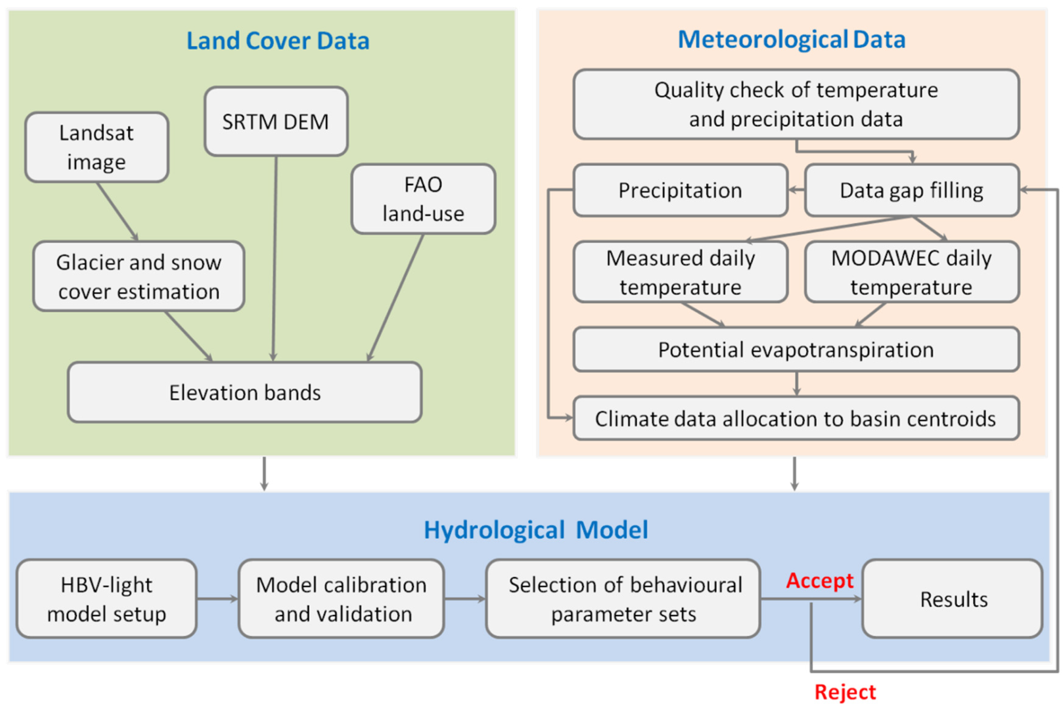
Widespread data scarcity cannot be gap-filled in a way that the output enables local water managements to rely on the synthesized data for the decisions in water allocation to users. Thus, results from synthesizing regional scale data with larger gaps may not be overstated. However, even rough estimations on the potential direction of change are highly appreciated by stakeholders and decision-makers, because water resources are so vulnerable in this area of the world. Hence, the scope of the present work was to develop an approach that can facilitate hydrological modeling of water resource availability under current climatic conditions based on a number of limited data sets (
Figure 3).
Our straightforward approach to hydrological modeling agrees well with suggestions by [
27,
28] and takes into account a number of performance criteria (Nash-Sutcliffe efficiency for high and log-transformed flow, and difference in annual water balance), and provides a meaningful representation of hydrological processes, the transformation of behavioral parameter sets in time (validation), and a sensitivity analysis of the model’s parameters. We selected the four river catchments with the most complete data and tested hydrological model performance given these aspects. Moreover, we tested MODAWEC weather generator for its applicability in the study region. MODAWEC converts monthly temperature data into daily values since only several weather stations are available at daily resolution (
Figure 2). To decide whether or not MODAWEC can be used for research on the other 15 catchments of the valley, the results of simulated hydrological outputs were compared, in terms of results from the two databases representing either generated or measured temperature (
Figure 3).
Figure 3.
Schematic representation of the selected model approach.
Figure 3.
Schematic representation of the selected model approach.
Preference was given to a lumped hydrological model for the hydrological simulation because of the limited quality of forcing data,
i.e., referring to the completeness of observed daily meteorological data for the study period. Amongst others, models from the HBV (Hydrologiska Byråns Vattenavdelning) family have proven to provide reliable results for mountainous catchments of Central, East and South Asia, and have recently been used for climate change impact studies in the region [
29,
30,
31,
32,
33,
34,
35]. We used the recently upgraded version of the HBV-light model for the water balance investigation of the Ferghana Valley, because this version is capable of simulating glacial melt [
36,
37]. We used a Monte Carlo approach to investigate the effect of model parameter uncertainty [
38,
39], which is only one part of the global model uncertainty that can arise from errors in input data, the model parameters, or the model structure [
38,
40,
41,
42]. In addition, the influence of the input parameters on the model’s output was assessed using sensitivity analysis [
43,
44].
3. Results and Discussion
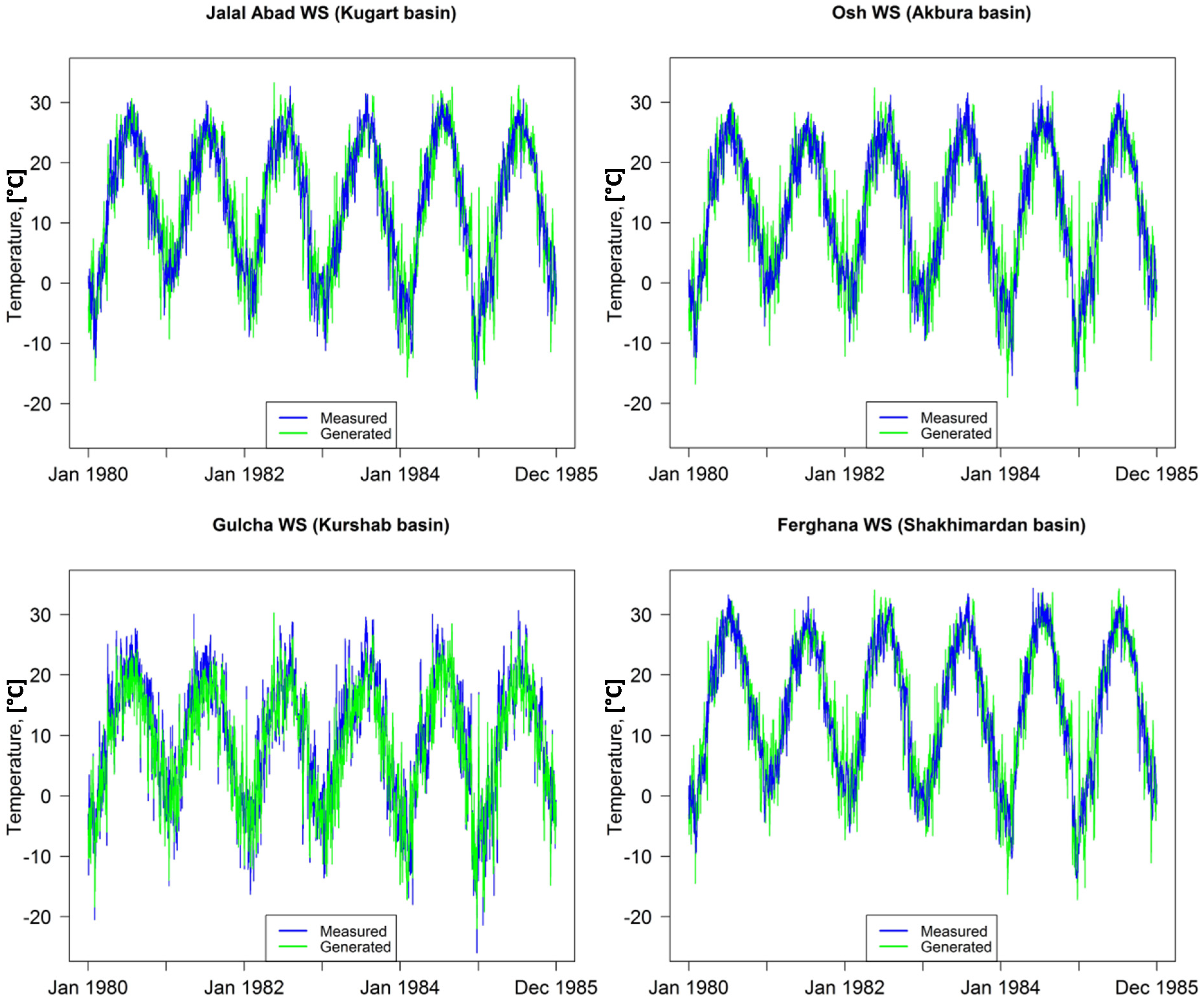
MODAWEC was tested using the database of the four studied catchments for its applicability in the region as the converter from monthly into daily temperatures. Results reveal that measured and generated mean maximum, minimum and average temperature data for corresponding weather stations (
Figure 2) are highly correlated (0.80 to 0.91).
Figure 6 shows generated and measured average temperature values at the four corresponding weather stations of the studied basins. Thus, the generator is capable of representing the main features and fluctuations that are similar to the observed temperatures.
Figure 6.
Time series plots of generated and measured temperature at the corresponding weather stations (WS) of the four studied river catchments.
Figure 6.
Time series plots of generated and measured temperature at the corresponding weather stations (WS) of the four studied river catchments.
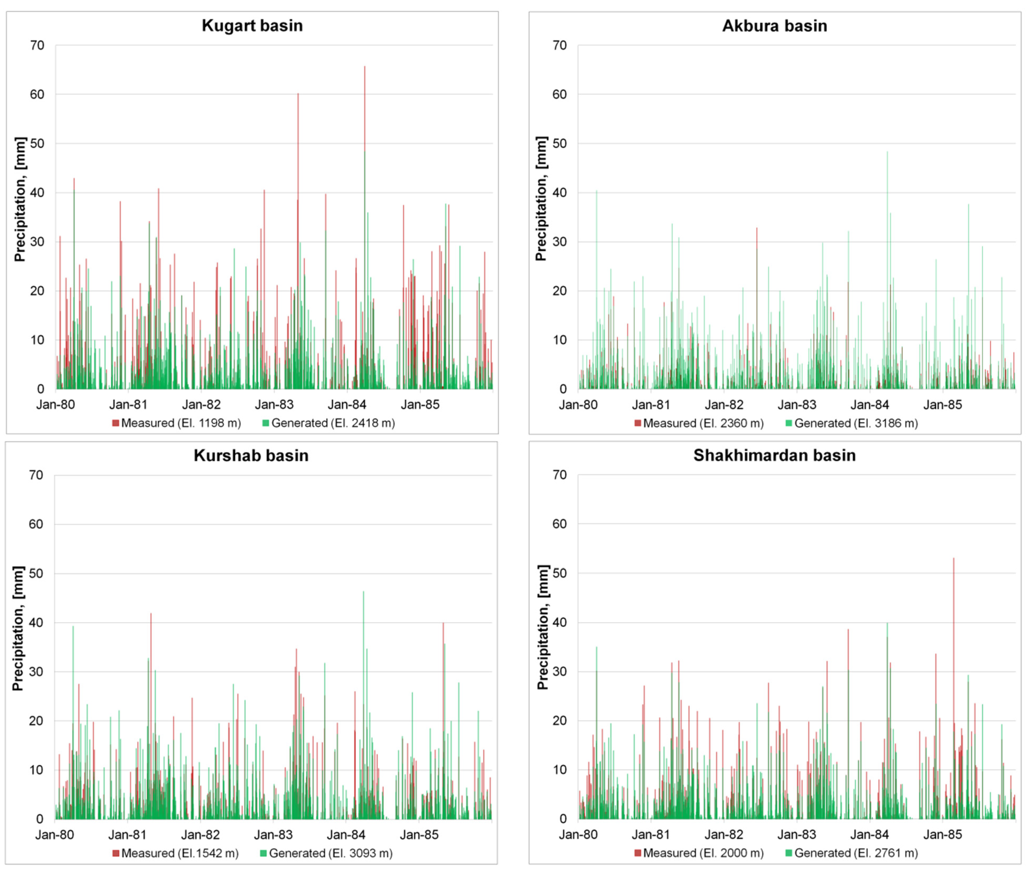
The corrected precipitation for the mean elevations of the studied catchments using MLR method and measured precipitation at the neighbor stations (
Figure 2) are presented in
Figure 7. The correlation coefficients vary from 0.65 in the Kugart river basin to 0.84 in the Shakhimardan river basin. It can be assumed that the calculated and measured precipitation time series are mostly similar and the main precipitation events occur in both cases at the same time. PET rates were calculated for the temperature data allocated to the centroids of each catchment. Correlation coefficients of PET calculated based on measured
versus MODAWEC temperatures vary from 0.84 to 0.92 for the researched basins.
Figure 7.
Time series plots of allocated precipitation to the centroids and measured precipitation at neighboring weather stations of the four river catchments.
Figure 7.
Time series plots of allocated precipitation to the centroids and measured precipitation at neighboring weather stations of the four river catchments.
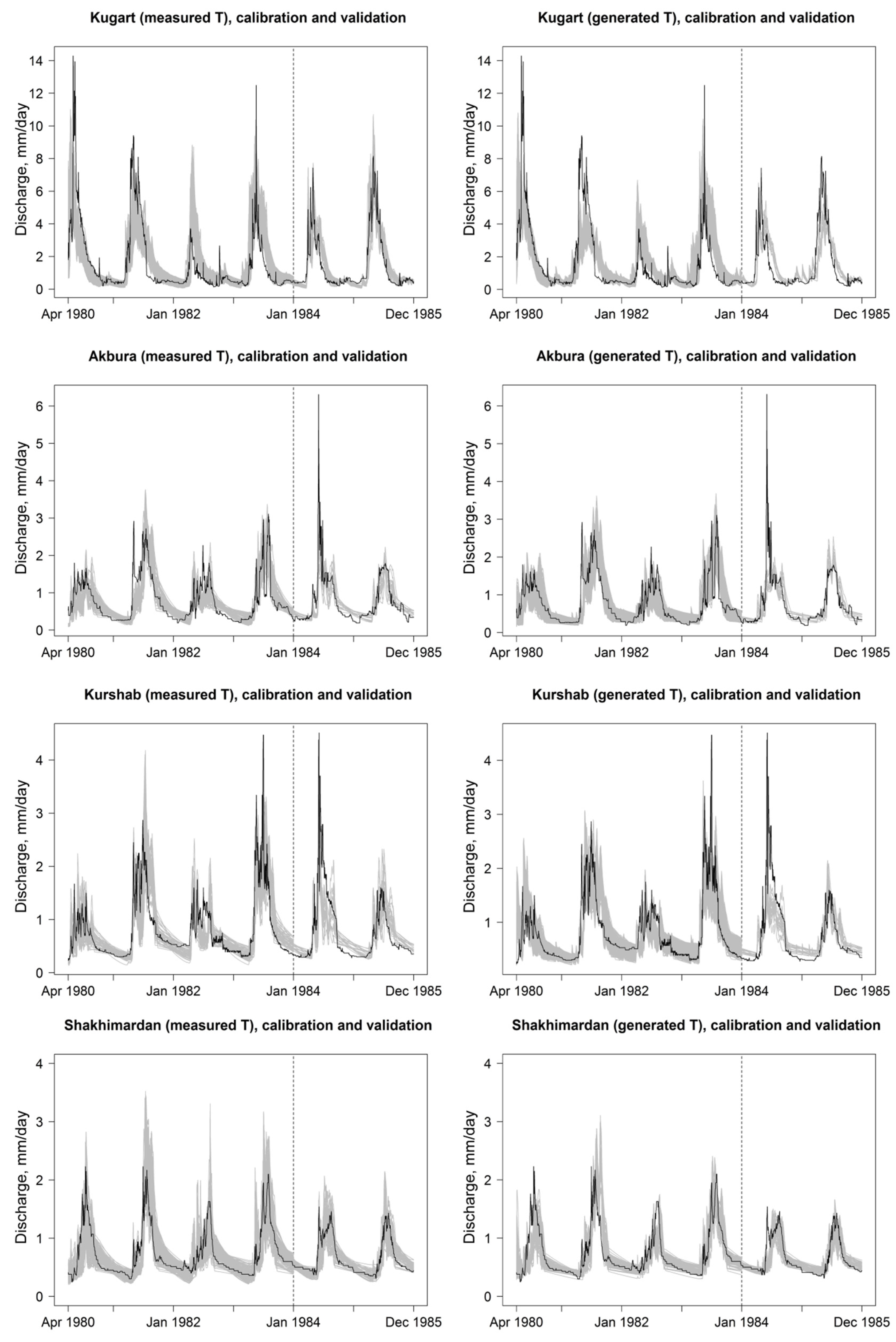
Results of the HBV-light model using both measured as well as MODAWEC input data for the calibration (1980–1983) and validation (1984–1985) period for the four different catchments are presented in
Table 4. In general, the HBV-light model is able to replicate the main peaks of discharge (NSE = 0.50–0.88) and simulate the base flow (NSE
log = 0.50–0.85) in the study area (
Figure 8). Higher NSE coefficients were often found for the validation than the calibration period. Similarly, the coefficient of determination (
R2) is higher for the validation (0.51–0.89) than the calibration (0.50–0.79) period. Some extreme discharge peaks are underestimated throughout all catchments, which is mainly attributable to an underestimation of snowmelt in late spring or early summer. From a visual inspection of hydrographs (
Figure 8) as well as from the statistical performance criteria (
Table 4) we did not find large differences between MODAWEC and measured temperature data-driven HBV-light simulations. Even though in some cases (e.g., Shakhimardan) the NSE dropped slightly, there were other cases where efficiency even increased (e.g., NSE
log for Akbura). For three of the four catchments the number of overall accepted model runs during calibration period increased when MODAWEC data were used.
Overall, the simulation of hydrological fluxes using HBV-light in combination with MODAWEC input data provided encouraging results, which suggests that using MODAWEC derived data represents a suitable method for water balance assessment in the data-scarce region. The MODAWEC weather generator was also used successfully as pre-processing tool for environmental modeling including the EPIC (Environmental Policy Integrated Climate) model [
65]. In the same study, crop yield and evapotranspiration were similar using measured and generated daily meteorological data. Various other studies employed MODAWEC and report acceptable to very good results (NSE = 0.55–0.93) [
81,
82,
83,
84].
Table 4.
Results of calibration and validation of the HBV-light model using allocated measured and generated temperature data, and MLR-calculated precipitation of the four pilot catchments.
Table 4.
Results of calibration and validation of the HBV-light model using allocated measured and generated temperature data, and MLR-calculated precipitation of the four pilot catchments.
| Goodness-of-Fit | Calibration, Allocated Measured Data | Validation | Calibration, Allocated Generated Temp. Data (MODAWEC) | Validation |
|---|
| 1980–1983 | 1984–1985 | 1980–1983 | 1984–1985 |
|---|
| Kugart river basin |
| No. Parameter sets | 2556 | 47 | 6973 | 14 |
| NSE | 0.50–0.63 | 0.50–0.88 | 0.50–0.61 | 0.50–0.65 |
| NSE_log | 0.50–0.71 | 0.50–0.77 | 0.50–0.69 | 0.50–0.67 |
| R2 | 0.50–0.65 | 0.65–0.89 | 0.50–0.63 | 0.54–0.65 |
| Cumulative mean difference, mm | −20 to 20 | −20 to 6 | −20 to 20 | −20 to 8 |
| Akbura river basin |
| No. Parameter sets | 79 | 14 | 540 | 12 |
| NSE | 0.50–0.61 | 0.50–0.68 | 0.50–0.65 | 0.50–0.60 |
| NSE_log | 0.50–0.72 | 0.50–0.72 | 0.50–0.77 | 0.50–0.77 |
| R2 | 0.50–0.67 | 0.51–0.72 | 0.50–0.69 | 0.52–0.61 |
| Cumulative mean difference, mm | −20 to 20 | −20 to 19 | −20 to 20 | 2 to 19 |
| Kurshab river basin |
| No. Parameter sets | 55 | 19 | 449 | 18 |
| NSE | 0.50–0.65 | 0.50–0.65 | 0.50–0.66 | 0.50–0.58 |
| NSE_log | 0.50–0.71 | 0.50–0.81 | 0.50–0.71 | 0.50–0.76 |
| R2 | 0.51–0.68 | 0.52–0.70 | 0.50–0.66 | 0.54–0.69 |
| Cumulative mean difference, mm | −20 to 20 | −17 to 18 | −20 to 20 | −1 to 20 |
| Shakhimardan river basin |
| No. Parameter sets | 174 | 66 | 102 | 64 |
| NSE | 0.50–0.70 | 0.50–0.80 | 0.50–0.64 | 0.50–0.80 |
| NSE_log | 0.50–0.76 | 0.50–0.85 | 0.50–0.77 | 0.50–0.85 |
| R2 | 0.51–0.79 | 0.52–0.87 | 0.53–0.73 | 0.52–0.82 |
| Cumulative mean difference, mm | −20 to 20 | −20 to 19 | −20 to 20 | −17 to 20 |
Figure 8.
Observed (black line) and simulated (grey lines) discharge series for calibration and validation periods (separated by vertical dashed line) using allocated measured (left) and generated (right) temperature and precipitation data for the studied basins.
Figure 8.
Observed (black line) and simulated (grey lines) discharge series for calibration and validation periods (separated by vertical dashed line) using allocated measured (left) and generated (right) temperature and precipitation data for the studied basins.
Furthermore, the results show that HBV-light is an acceptable model to be used in the data scarce application of this study. Similar results for HBV-light have been found by others with NSE ranging between 0.49 and 0.85 in catchments of Central Asia, China, Central and Northern Europe, and Ethiopia [
2,
36,
39,
69,
85]. For mountainous catchments in the Himalayan and Central Tibetan Plateau, reported NSE values also vary in comparable ranges of 0.43–0.95 [
86] and 0.67–0.82 [
33], respectively. Different versions of the HBV models were applied in Central Asia. The HBV-ETH model was used in glacial catchments of Kyrgyzstan [
34] and in the Amu-Darya River basin in Tajikistan [
87]. Their results showed accurate runoff simulations with NSE coefficients between 0.83–0.89 and 0.86–0.94, respectively. For the HBV-IWS version applied in Uzbekistan (Chirchik River) NSE ranged between 0.69 and 0.94 [
88].
The reasons for differences in model performance are manifold, including divergent model structures (HBV-light versus HBV-ETH and HBV-IWS), varying geographical and meteorological conditions (i.e., a direct comparison of model performance is only valid if different model structures are applied to the same catchment and same boundary conditions), length and split of calibration and validation periods, methods of calibration, and types of efficiency criteria (we used three validation criteria that must be met by the HBV-light model at the same time, while others used single or different combinations of performance criteria).
The majority of the HBV-light model’s parameters were calibrated within moderate parameter ranges comparable to other studies [
36,
38,
39] (
Table 5 and
Table 6). The SFCF (Snowfall correction factor) and CFMAX (Degree-day factor) parameters were calibrated within wider ranges. SFCF depends on wind speed and temperature, the greater the wind speed, the greater the SFCF [
89,
90]. In addition, [
91] showed that the gauge catch efficiency ranges between 23% and 106% due to gauge type and wind speed. Thus, SFCF can reach large values of 1.5 or greater, which was also shown by others [
36,
87,
89,
92,
93]. CFMAX is low in forested areas [
94] and high in glacial regions and zones with high elevation and incoming solar radiation [
95]. For example, high values of CFMAX in the Himalayan ranged from 7 to 37 mm·day
−1∙°C
−1 on debris cover, and 17 mm·day
−1∙°C
−1 over pure ice [
96,
97]. Other findings of CFMAX were 10 mm·day
−1∙°C
−1 in Austria and Switzerland [
36] and 14 mm·day
−1∙°C
−1 for west China [
98]. Reference [
95] reviewed a number of studies and reported maxima of up to 20 mm·day
−1∙°C
−1 in Sweden and Greenland. Overall, the ranges used in the present study are relatively high but still in agreement with other published values.
Table 5.
Description of model parameters and their ranges for allocated measured temperature data and calculated precipitation of the four studied catchments.
Table 5.
Description of model parameters and their ranges for allocated measured temperature data and calculated precipitation of the four studied catchments.
| Parameter | Description/Unit | Kugart River | Akbura River | Kurshab River | Shakhimardan River |
|---|
| Min | Max | Min | Max | Min | Max | Min | Max |
|---|
| Snow Routine | | | | | | | | | |
| TT | Threshold temperature/°C | −0.5 | 1 | −0.5 | 0.5 | −0.5 | 0.5 | −0.5 | 0.5 |
| CFMAX | Degree-day factor/mm·°C−1·d−1 | 2 | 15 | 2 | 15 | 2 | 15 | 1 | 12 |
| SFCF | Snowfall correction factor/- | 0.5 | 3 | 0.1 | 1.5 | 0.1 | 1.5 | 0.3 | 1 |
| CWH | Water holding capacity/- | 0.2 | 0.5 | 0.05 | 0.5 | 0.05 | 0.5 | 0.2 | 0.5 |
| CFR | Refreezing coefficient/- | 0.2 | 0.9 | 0.05 | 0.6 | 0.05 | 0.6 | 0.05 | 0.5 |
| CFGlacier | Glacier correction factor/- | - | - | 0.9 | 1.2 | 0.8 | 1.2 | 0.4 | 1.3 |
| CFSlope | Slope correction factor/- | - | - | 1 | 1.1 | 1 | 1.1 | 0.6 | 1.3 |
| Soil and evaporation Routine | |
| FC | Field capacity/mm | 50 | 350 | 100 | 350 | 50 | 350 | 250 | 550 |
| LP | Threshold for reduction of evaporation/- | 0.4 | 1 | 0.4 | 1 | 0.3 | 1 | 0.3 | 1 |
| BETA | Shape coefficient/- | 0.3 | 3 | 1.5 | 2.5 | 1 | 5 | 1.5 | 5 |
| Ground water and response routine | |
| K1 | Recession coefficient (upper box)/d−1 | 0.001 | 0.03 | 0.01 | 0.04 | 0.01 | 0.04 | 0.02 | 0.1 |
| K2 | Recession coefficient (lower box)/d−1 | 0.005 | 0.03 | 0.001 | 0.01 | 0.001 | 0.01 | 0.001 | 0.01 |
| PERC | Maximal flow from upper to lower box/mm·d−1 | >0 | 4 | 1 | 4.5 | 1 | 4.5 | >0 | 4 |
| MAXBAS | Routing, length of weighting function/d | 1 | 5 | 1 | 5 | 1 | 5 | 1 | 5 |
Table 6.
Parameter ranges for the MODAWEC-generated temperature data allocated to the centroids.
Table 6.
Parameter ranges for the MODAWEC-generated temperature data allocated to the centroids.
| Parameter | Kugart River | Akbura River | Kurshab River | Shakhimardan River |
|---|
| Min | Max | Min | Max | Min | Max | Min | Max |
|---|
| Snow routine | | | | | | | | |
| TT * | −0.5 | 0.5 | −0.5 | 0.5 | −0.5 | 0.5 | −0.5 | 0.5 |
| CFMAX | 2 | 15 | 1 | 15 | 2 | 12 | 1 | 12 |
| SFCF | 1 | 3 | 0.1 | 1.5 | 0.5 | 1.5 | 0.4 | 1.2 |
| CWH | 0.2 | 0.5 | 0.1 | 0.5 | 0.05 | 0.5 | 0.1 | 0.5 |
| CFR | 0.2 | 0.7 | 0.3 | 0.5 | 0.05 | 0.6 | 0.05 | 0.5 |
| CFGlacier | - | - | 0.9 | 1.2 | 0.9 | 1.2 | 0.5 | 1.4 |
| CFSlope | - | - | 1 | 1.06 | 1 | 1.1 | 0.6 | 1.3 |
| Soil and evaporation routine | | | |
| FC | 150 | 350 | 50 | 350 | 150 | 350 | 250 | 550 |
| LP | 0.5 | 1 | 0.4 | 0.7 | 0.5 | 0.9 | 0.3 | 1 |
| BETA | 0.3 | 2.5 | 3 | 5 | 1.5 | 2.5 | 2 | 7 |
| Groundwater and response routine | | | |
| K1 | 0.01 | 0.02 | 0.01 | 0.03 | 0.01 | 0.04 | 0.02 | 0.06 |
| K2 | 0.009 | 0.03 | 0.001 | 0.003 | 0.001 | 0.005 | 0.001 | 0.003 |
| PERC | >0 | 4 | 0.5 | 3 | >0 | 3 | >0 | 2 |
| MAXBAS | 1 | 3 | 1 | 4 | 1 | 5 | 1 | 4 |
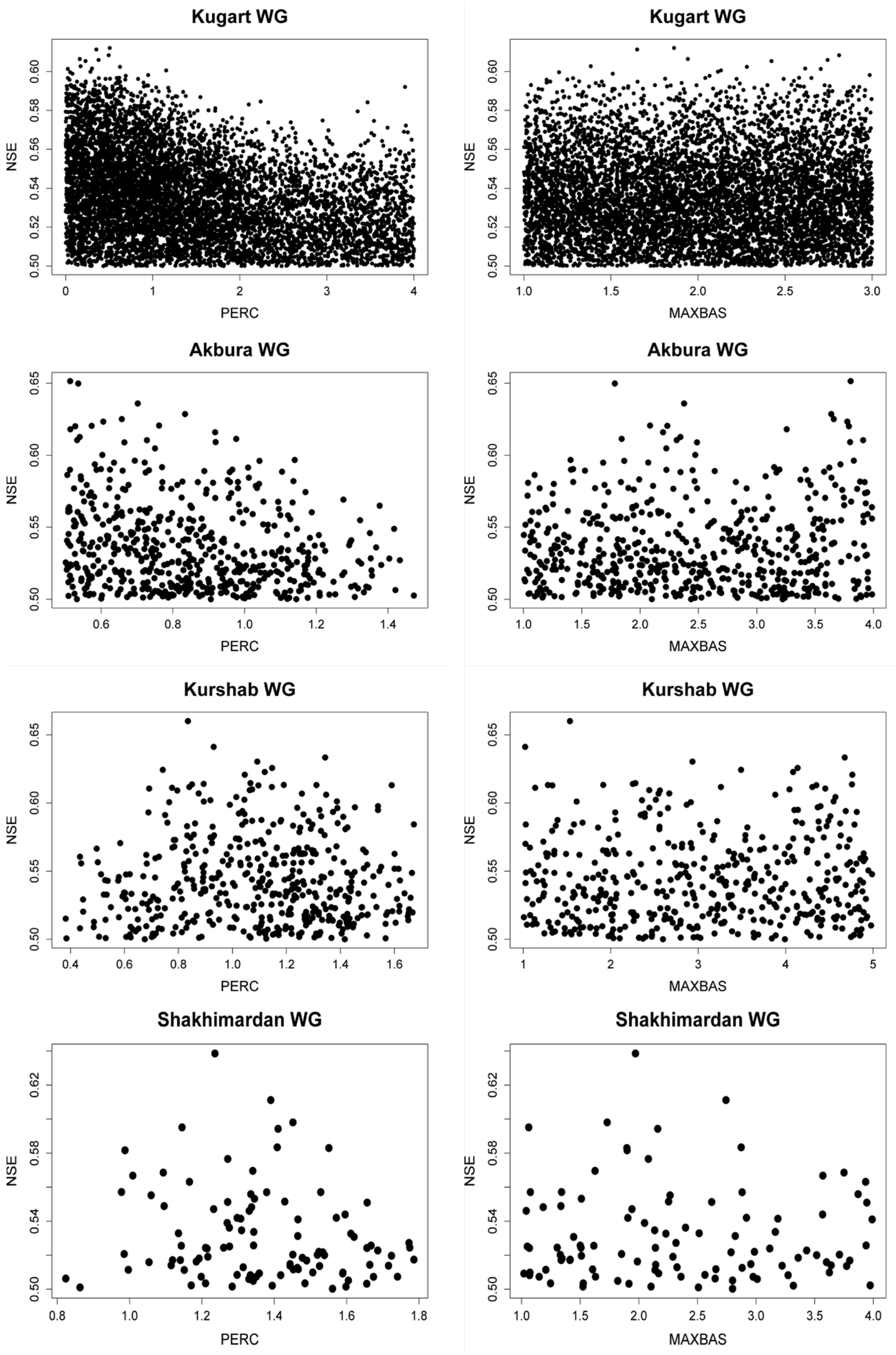
Scatter plots for all parameters and NSE coefficients of the four catchments were drawn using results of the MODAWEC-driven HBV-light application to perform sensitivity analysis, as suggested by [
40,
44,
99]. Examples of two parameters for the studied basins are presented in
Figure 9. While PERC was rather constrained for Kugart and Akbura, it was less clear to find optimal parameter values for PERC in the Kurshab and Shakimardan catchments. MAXBAS on the other hand was not constrained for any of the four catchments. We further tested the importance of model parameters for the model outputs by a regression analysis [
40,
100], for which results are given in
Table 7. The importance of the predictors indicates the influence of the parameters on the model’s efficiency coefficients (NSE, NSE
log). The regression technique is used among other studies for evaluation of parameter influence on the results [
44,
101,
102]. In addition, [
44] noticed that parameter sensitivity analyses contribute to output uncertainty reduction and identifiability of parameters which require additional research. The stepwise regression models were calculated using dependency of NSE and NSE
log coefficients on HBV-light parameters accordingly for different vegetation zones [
103], since the snow and soil routine are calculated individually for each vegetation zone [
55]. The adjusted coefficients of determination for the NSE and NSE
log vary from 0.25 to 0.86 and from 0.26 to 0.98 (
Table 7). In general, the adjusted coefficients of determination are higher in validation, which indicates better explanation of the variability in the model’s efficiency coefficients because of parameter combination [
104]. The total number of parameters in the regression models varies from 2 to 18 (
Table 7). The standardized beta coefficients are included in the table only if they are statistically significant (
p-value ≤ 0.05). The beta values determine how strongly the parameters affect the dependent variable. The higher the beta value the greater the contribution of a parameter to model results [
104]. In addition, [
105,
106,
107] reported that the standardized beta coefficients vary from −1 to 1 and show the decrease or increase in the dependent variable accordingly. Thus, in the studied catchments PERC and K1 have significant influences on the goodness-of-fit coefficients with inverse relationship (0.412–0.936) and positive direction (0.548–0.730) accordingly. In general, the following parameters are relevant for high-flow simulations: PERC, CFMAX, SFCF, CWH, K1, and LP. The most important parameters responsible for recession flows are PERC, CFMAX and TT, followed by K1, Alpha, LP and CWH.
Reference [
66] carried out a parameter sensitivity analysis of HBV-light in Sweden and reported that SFCF, MAXBAS, CFMAX and K1 were the most sensitive parameters. [
108] applied HBV-light in North-Eastern Germany, and revealed that the most sensitive parameters were SFCF, CFMAX, FC (Field capacity), LP (Limit for potential evaporation), BETA (Shape coefficient), Alpha, K1 and MAXBAS (Length of triangular weighting function). In an Ethiopian case study [
85] derived FC, PERC, BETA and K2 as most sensitive, while K1, MAXBAS, PERC, FC, BETA and LP proved to be relevant for a US catchment [
109]. Reference [
110] used the HBV-96 model in four different climate zones and found out that the most important parameters for the model are the routing parameter MAXBAS and the recession coefficient KHQ, whereas FC and PERC were insensitive. Obviously, there is not a single most important parameter for HBV applications, but MAXBAS was most often found to be sensitive followed by FC, BETA, K1, as well as LP, SFCF and CFMAX. Surprisingly, MAXBAS was a rather insensitive parameter in our model application. We explain this by the importance of snow and glacial melt that drives the hydrology in the studied catchments.
Finally, we investigated the interaction between the parameters using correlation analysis [
111]. Correlations between parameters were analyzed for each catchment with both measured and MODAWEC-generated time series. Instead of many pages of tables,
Table 8 summarizes the ranges of all correlation coefficients for each catchment. The linear relationship among parameters was mainly weak. Moderate correlations (0.4–0.6) were mainly found between PERC and K2, Alpha and K1, SFCF with CWH (Water holding capacity), BETA, LP, and CFMAX with SFCF, CFGlacier, TT and CFR for the studied catchments. These results indicate a large equifinality of parameters [
71] and many unconstrained parameters.
Figure 9.
Examples of scatter plots with sensitive (PERC) and insensitive (MAXBAS) parameters for the four studied catchments with MODAWEC generated temperature data.
Figure 9.
Examples of scatter plots with sensitive (PERC) and insensitive (MAXBAS) parameters for the four studied catchments with MODAWEC generated temperature data.
Table 7.
Contribution of parameters in HBV-light model for the four studied catchments based on the adjusted coefficient of determination and standardized beta coefficient (VZ * = vegetation zone).
Table 7.
Contribution of parameters in HBV-light model for the four studied catchments based on the adjusted coefficient of determination and standardized beta coefficient (VZ * = vegetation zone).
| | Kugart WG | Akbura WG | Kurshab WG | Shakhimardan WG |
|---|
| Calibration | Validation | Calibration | Validation | Calibration | Validation | Calibration | Validation |
|---|
| Dependent | NSE | NSElog | NSE | NSElog | NSE | NSElog | NSE | NSElog | NSE | NSElog | NSE | NSElog | NSE | NSElog | NSE | NSElog |
|---|
| R2 adjusted | 0.25 | 0.38 | 0.75 | 0.52 | 0.28 | 0.77 | 0.86 | 0.98 | 0.3 | 0.44 | 0.64 | 0.95 | 0.29 | 0.26 | 0.76 | 0.86 |
|---|
| No | Parameters | Standardized Beta Coefficient |
|---|
| 1 | PERC | −0.412 | −0.368 | | | −0.201 | −0.826 | | −0.493 | −0.127 | −0.579 | −0.851 | −0.887 | | −0.432 | −0.819 | −0.936 |
| 2 | Alpha | | 0.326 | | | | | −0.453 | −0.382 | | −0.116 | | | | | | |
| 3 | K1 | 0.029 | 0.195 | 0.73 | 0.508 | | −0.067 | 0.548 | | −0.183 | −0.258 | | | | | | |
| 4 | K2 | 0.166 | 0.027 | | | −0.201 | | | | −0.090 | 0.095 | | | | | | 0.133 |
| 5 | MAXBAS | | −0.019 | | | | | | | | | | | | | | |
| 6 | TT_VZ*1 | −0.085 | −0.120 | −0.598 | −0.646 | | | | | −0.088 | | | | | | | |
| 7 | CFMAX_VZ1 | 0.029 | 0.407 | | | | | | | | | | | | | | |
| 8 | SFCF_VZ1 | 0.043 | −0.155 | | | | | | | 0.186 | | | | | | | |
| 9 | CFR_VZ1 | −0.042 | −0.027 | | | | | | −0.134 | 0.116 | 0.089 | | | | | | |
| 10 | CWH_VZ1 | −0.043 | −0.047 | | | | | | | | | | | | | | |
| 11 | CFGlacier_VZ1 | − | − | − | − | | | | | | | −0.515 | | 0.229 | | | |
| 12 | CFSlope_VZ1 | − | − | − | − | | | | | | −0.072 | | | | | | |
| 13 | FC_VZ1 | | −0.026 | | | | | | | −0.095 | | | | | | | |
| 14 | LP_VZ1 | 0.06 | | | | | | | | | | | 0.164 | | −0.258 | −0.193 | −0.132 |
| 15 | BETA_VZ1 | | 0.073 | | | | | | | 0.085 | | −0.381 | | | | | |
| 16 | TT_VZ2 | −0.046 | −0.062 | | | −0.173 | | | | −0.275 | −0.073 | | | | | | |
| 17 | CFMAX_VZ2 | −0.297 | 0.068 | | | 0.162 | −0.103 | −0.403 | −0.549 | 0.353 | | | | | | | |
| 18 | SFCF_VZ2 | 0.231 | 0.116 | | | −0.194 | | | | | | | | | | | |
| 19 | CFR_VZ2 | −0.076 | | | | | | | | | | | | | | | |
| 20 | CWH_VZ2 | 0.036 | | | | −0.174 | | | | −0.357 | −0.135 | | | | | | |
| 21 | CFGlacier_VZ2 | − | − | − | − | | | | | | | | | | | | |
| 22 | CFSlope_VZ2 | − | − | − | − | | | | | | | | | | | | |
| 23 | FC_VZ2 | | −0.062 | | | −0.087 | −0.103 | | | −0.206 | | | | | | | |
| 24 | LP_VZ2 | 0.148 | | | | | 0.077 | | | −0.128 | −0.131 | | | | | | |
| 25 | BETA_VZ2 | −0.180 | 0.175 | | | | | | | 0.1 | 0.11 | | | | | | |
| 26 | TT_VZ3 | − | − | − | − | 0.247 | | | | | | | | | | | |
| 27 | CFMAX_VZ3 | − | − | − | − | −0.400 | | | | −0.258 | −0.079 | | | | | 0.449 | 0.341 |
| 28 | SFCF_VZ3 | − | − | − | − | 0.335 | −0.050 | | | 0.171 | | | −0.129 | 0.293 | | | |
| 29 | CFR_VZ3 | − | − | − | − | | | | | | | | | −0.198 | | | |
| 30 | CWH_VZ3 | − | − | − | − | 0.27 | −0.097 | | | | | | | | | | |
| 31 | CFGlacier_VZ3 | − | − | − | − | | | | | | | | | | | | |
| 32 | CFSlope_VZ3 | − | − | − | − | | | | | | | | | | | | |
| 33 | FC_VZ3 | − | − | − | − | | −0.064 | | | −0.112 | −0.099 | | | | | | |
| 34 | LP_VZ3 | − | − | − | − | | | | 0.166 | −0.096 | −0.092 | | | 0.395 | | | |
| 35 | BETA_VZ3 | − | − | − | − | | 0.045 | | | | | | | 0.202 | | | |
| Total | 16 | 17 | 2 | 2 | 11 | 9 | 3 | 5 | 18 | 13 | 3 | 3 | 5 | 2 | 3 | 4 |
Table 8.
The range of correlation coefficients among the parameters generated using the MC method for the studied basins. NA = not available, parameter is only needed for glaciered catchments.
Table 8.
The range of correlation coefficients among the parameters generated using the MC method for the studied basins. NA = not available, parameter is only needed for glaciered catchments.
| Parameters | Akbura | Akbura_WG | Kugart | Kugart_WG | Kurshab | Kurshab_WG | Shakhimardan | Shakhimardan_WG |
|---|
| max | min | max | min | max | min | max | Min | max | min | max | min | max | min | max | min |
|---|
| PERC | 0.4 | −0.2 | 0.4 | −0.1 | 0.3 | −0.1 | 0.4 | −0.1 | 0.3 | −0.2 | 0.3 | −0.1 | 0.3 | −0.1 | 0.4 | −0.3 |
| Alpha | 0.2 | −0.3 | 0.1 | −0.1 | 0.1 | −0.6 | 0.0 | −0.3 | 0.3 | −0.3 | 0.1 | −0.4 | 0.1 | −0.1 | 0.3 | −0.2 |
| K1 | 0.3 | −0.3 | 0.1 | −0.2 | 0.1 | −0.2 | 0.0 | −0.1 | 0.2 | −0.3 | 0.1 | −0.1 | 0.3 | −0.2 | 0.3 | −0.2 |
| K2 | 0.2 | −0.3 | 0.1 | −0.3 | 0.2 | −0.3 | 0.1 | 0.0 | 0.2 | −0.3 | 0.1 | −0.3 | 0.3 | −0.3 | 0.1 | −0.3 |
| MAXBAS | 0.2 | −0.2 | 0.1 | −0.1 | 0.0 | 0.0 | 0.0 | 0.0 | 0.3 | −0.3 | 0.1 | −0.1 | 0.2 | −0.2 | 0.2 | −0.1 |
| TT | 0.3 | −0.3 | 0.1 | 0.0 | 0.0 | −0.1 | 0.0 | 0.0 | 0.3 | −0.3 | 0.1 | −0.1 | 0.2 | −0.2 | 0.2 | −0.2 |
| CFMAX | 0.4 | −0.2 | 0.1 | −0.1 | 0.1 | −0.1 | 0.1 | −0.1 | 0.3 | −0.3 | 0.1 | −0.1 | 0.2 | −0.1 | 0.2 | −0.2 |
| SFCF | 0.2 | −0.3 | 0.1 | −0.1 | 0.1 | −0.6 | 0.3 | −0.3 | 0.5 | −0.6 | 0.1 | −0.2 | 0.2 | −0.3 | 0.4 | −0.1 |
| CFR | 0.2 | −0.1 | 0.1 | −0.1 | 0.0 | −0.1 | 0.0 | 0.0 | 0.2 | −0.4 | 0.1 | −0.1 | 0.2 | −0.1 | 0.2 | −0.1 |
| CWH | 0.2 | −0.2 | 0.1 | −0.1 | 0.0 | 0.0 | 0.0 | 0.0 | 0.2 | −0.3 | 0.1 | −0.1 | 0.1 | −0.1 | 0.2 | −0.1 |
| CFGlacier | 0.2 | −0.2 | 0.1 | 0.0 | NA | NA | NA | NA | 0.4 | −0.4 | 0.1 | −0.1 | 0.1 | −0.1 | 0.2 | −0.3 |
| CFSlope | 0.2 | −0.3 | 0.1 | −0.1 | NA | NA | NA | NA | 0.4 | −0.2 | 0.1 | −0.1 | 0.1 | −0.1 | 0.1 | −0.1 |
| FC | 0.2 | −0.2 | 0.1 | −0.1 | 0.0 | 0.0 | 0.0 | 0.0 | 0.2 | −0.2 | 0.1 | −0.1 | 0.1 | −0.2 | 0.2 | −0.1 |
| LP | 0.2 | −0.3 | 0.1 | −0.1 | 0.1 | 0.0 | 0.1 | 0.0 | 0.3 | −0.3 | 0.1 | −0.2 | 0.2 | −0.2 | 0.3 | −0.2 |
| BETA | 0.1 | −0.2 | 0.1 | −0.1 | 0.0 | −0.1 | 0.1 | −0.1 | 0.2 | −0.3 | 0.1 | 0.0 | 0.1 | −0.1 | 0.2 | −0.2 |


