Article

A Proposed Model to Assess and Map Irrigation Water Well Suitability Using Geospatial Analysis

Soil and Water Department, Suez Canal University, Ismailia 41522, Egypt
Water 2012, 4(3), 545-567; https://doi.org/10.3390/w4030545
Submission received: 24 April 2012 / Revised: 25 June 2012 / Accepted: 10 July 2012 / Published: 24 July 2012

Abstract

:
Assessing the vulnerability of groundwater is the first step toward careful management of water resources to avoid or, at least, to minimize impacts on agriculture. The objective of this study was to propose a simple method to assess the groundwater quality and to map its spatial variation in terms of suitability for irrigation in the Darb El-Arbaein area, Southwestern Desert, Egypt. Thirty-six surveyed wells were used to assess and map the groundwater quality. For calculating the Water Quality Index (WQI), a total of 20 (13 chemical, two physical, and five calculated) parameters were considered e.g., EC, pH, Cl, SAR, B, Zn, iron, Mn, Pb and Cd. The results of analyses were used to propose a water quality model. The different water quality maps were produced using GIS software. The results show that three water samples fall into the moderate WQI. Most of the samples (26) fall into the unsuitable WQI category. Seven samples fall into the suitable WQI category. Groundwater samples that fall into the low salinity hazard class and high WQI can be used for irrigation of most crops and the majority of soils. The WQI for the samples ranges from 47.9 to 88.6. The WQI distribution maps delineating an area of 266.66 ha are suitable for irrigation in villages (3,4) and areas of 382.35 ha are moderately suitability for villages (1,2). Since the final map shows the spatial distribution of irrigation water quality in the area, it is now much easier for a decision maker to assess the water quality for irrigation and to locate the most suitable site for drilling wells. The present study demonstrates high efficiency for GIS to analyze complex spatial data and groundwater quality mapping.

1. Introduction

Groundwater quality evaluation in developing countries has become a critical issue due to fresh water scarcity. The quality of groundwater is equally important as the quantity. Assessment of groundwater vulnerability to pollution is necessary for feasibility and development analysis, planning management, and land use decisions. Two major techniques for groundwater protection strategies are groundwater vulnerability assessment and groundwater quality mapping. Groundwater quality mapping is one of the major techniques, which provide information about water suitability for irrigation. Water Quality Index (WQI) is a very useful and efficient method for assessing the suitability of water quality and for communicating the information on the overall quality of water [1,2,3,4] to the concerned decision-makers. Many studies and projects have been conducted to assess water quality [5]. Shihab and Al-Rawi [6] and Al-Hussain [7] used WQI as a management tool for water quality of the Tigris River within Mosul city for different uses. Debels et al. [8] used a modified water quality index that is composed of physicochemical parameters for evaluating the quality status of a river in Central Chile. Numaan [9] established irrigation WQI for the Tigris River between Al-Sharqat and Alboajeel in Iraq. Bhatti and Latif [10] used a water quality index to assess the water quality of the Chenab River in Pakistan for irrigation use. Fulazzaky [11] assessed the status and the suitability of Citarum River water in Malaysia for agricultural use. Meireles et al. [12] classified the water quality in the the Acarau Basin, in the North of the state of Ceara, Brazil for irrigation use.
Pollution of water has become a health concern both in urban and rural areas [13]. Parameters that generally need to be considered for modeling WQI are for example EC, pH, B, Na, Cl and HCO3. Specific properties in water such as residual sodium carbonate (RSC) and sodium adsorption ratio (SAR) may be suitable or unsuitable for irrigation. The information on concentrations of some important heavy metals (Cu, Zn, Pb, Cr, and Cd) is necessary to assess its suitability for irrigation. Many studies have successfully used interpolation techniques of the ArcGIS Geostatistical tool [14,15,16]. Ordinary Kriging (OK) and lognormal Kriging were used to produce the spatial patterns of heavy metals and disjunctive Kriging was applied to quantify the probability of heavy metal concentrations higher than their guide values [17]. Geostatistical methods, Kriging and Co-Kriging, were applied to estimate the sodium adsorption ratio (SAR) in a 3,375 ha agricultural field [18].
The knowledge of irrigation water quality is critical to understand what management changes are necessary for long-term and short-term productivity, particularly for crops that are sensitive to changes in quality [19]. With an adequate database, GIS can be a powerful tool for assessing water quality, developing solutions for water resource problems, and it is a decision-making tool for agriculture development [20]. Despite the large number of studies regarding water quality index techniques, no complete assessment tool has been found in the literature that incorporates the crucial aspects of irrigational water quality analysis. Indexes based on specialist opinion and on statistical methods have some degree of subjectivity, because they depend on the choice of variables upon which the major indicators of water quality are built. Thus generalization is not acceptable due to special characteristics of each water system. Simple, objective, and interpretable methods that use the peculiar characteristics of water resources are necessary to simplify the analysis of water quality in the monitoring task.
The overall objective of the current study is “to propose a simple model to evaluate and map groundwater quality using Geostatistics in Darb El-Arbaein, Southwestern Desert, Egypt”. The purposes of this assessment are: (1) To evaluate and monitor the status of groundwater quality and assess its suitability for irrigation; (2) to determine the spatial distribution of groundwater quality parameters; and (3) to generate a groundwater quality map for the Darb El-Arbaein area. There is an urgent need to have a first-hand assessment of the groundwater quality in the Darb El-Arbaein area which has special significance and needs great attention of all concerned since it is the main source of domestic, irrigating and drinking water.

2. Materials and Methods

2.1. Study Area

Darb El-Arbaein, a historic desert track running between Sudan and Egypt and passing El-Kharga Oasis to Assuit, is geographically located between 30°21′56.7″–31°27′4.1″ E and 24°40′28.5″–23°40′31.6″ N, in Southwestern Desert, Egypt. Arid climatic conditions are dominant and rainfall is rare. The area is considered one of the horizontal extensions for settlement developments in the Western Desert, which aims at establishing a link between the South Valley Project and Al-Kharga Oasis. The current project aims at reclamation 4654 ha and digging 85 wells of 150–500 m depth.
The project “Development of Trans-Sahara camel route between the Sudan and Egypt (Darb El-Arbaein)” is intended to: (a) reduce camel mortality due to inadequacy of water and services on a 1500 km long route to markets; (b) promote regional camel trade and improve the economies of the region; and (c) motivate desert nomads to become more interested in camel breeding and marketing [21]. Groundwater is the only available source of water in the area. The assessment of agricultural potentiality in the Darb El-Arbaein area requires water resource evaluation. The general geology and geomorphology of the area studied are outlined in the geology of Egypt [22] which is a desertic plateau with vast flat expansions of rocky deep closed in depressions (
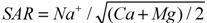
Figure 1). The greatest altitude is attained in the extreme southwestern corner where the general plateau character is disturbed by the great mountain Gebel Uweinat. The study area (Figure 1), which consists of four villages 1–4, encompasses around 5723.18 ha. The area of villages 1,2 is equal to 1933.45 ha, however; villages 3,4 have an area equal to 3789.73 ha.

2.2. Overall the Proposed Methodology

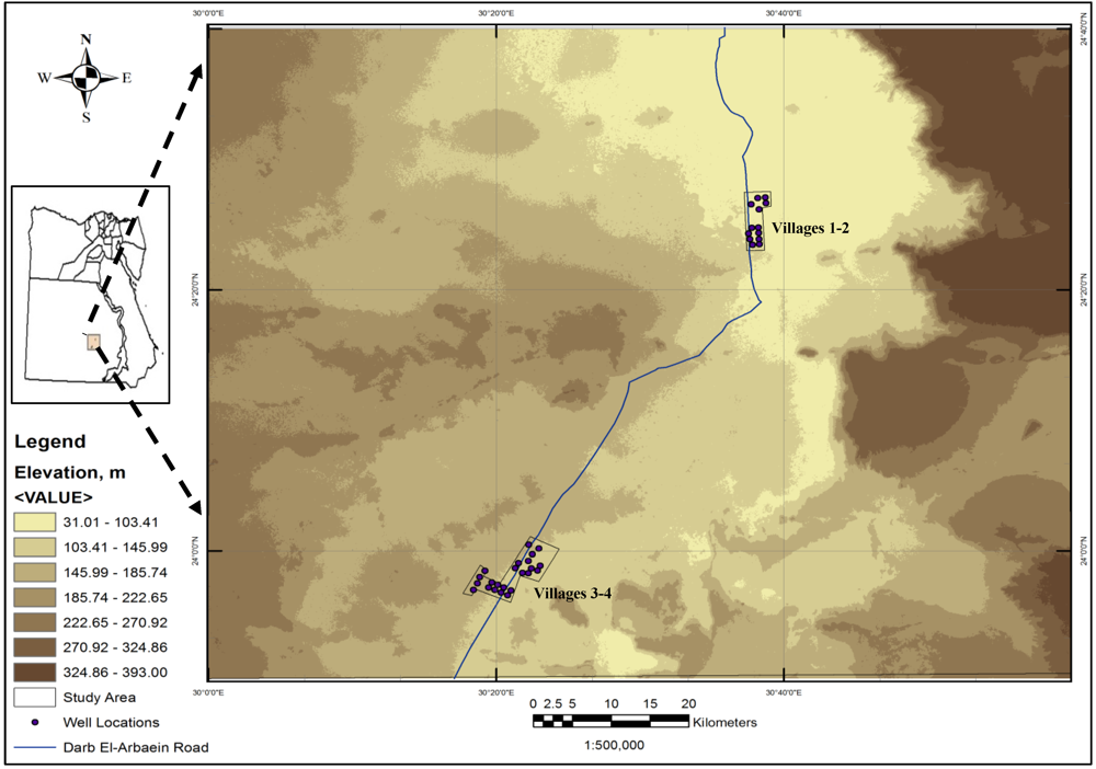
The methodology adopted for groundwater quality mapping using water quality data in the GIS environment is shown in Figure 2. The study was carried out with the help of four major components: input from remote sensing data, topographic sheets, groundwater quality data and data collected during field visits. In order to evaluate the quality of groundwater for irrigation in the Darb El-Arbaein area, 36 surveyed wells (13 in villages 1,2 and 23 in villages 3,4) with GPS (Garmin eTrex Venture HC) data were used to produce the evaluation map. The water samples were collected after 30 min of pumping to avoid stagnant and contaminated water. White plastic containers of 1 L capacity were rinsed out three to four times with sampling water. Then the containers were filled up to the brim and immediately sealed to avoid exposure to air [23]. The containers were labeled for identification and brought to the laboratory. The groundwater samples were analyzed for (pH, EC, Na+, Ca++, Mg++, B, Cl and HCO3-) irrigation purposes. Sodium Adsorption Ratio (SAR), Soluble Sodium Percentage (SSP) and Residual Sodium Carbonate (RSC) were calculated on some standard equations basis. These equations are as follows:
Water 04 00545 i001
Water 04 00545 i002
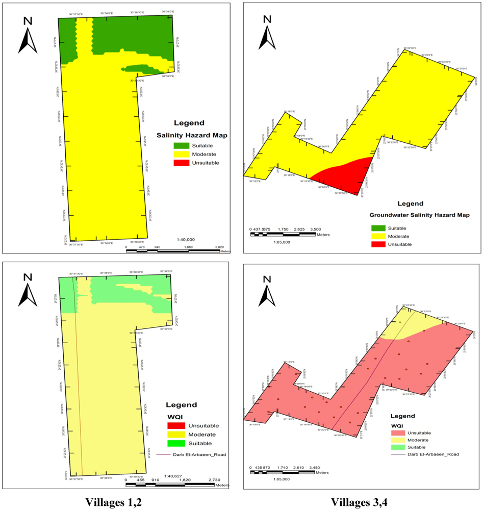
The concentrations of the heavy metals (Co, Fe, Pb, Ni, Cd, Zn and Cu) were determined using atomic absorption spectrophotometer. Area elevation and depth to water were also measured. Water quality maps were generated for different water properties and surfaces were interpolated using Kriging interpolation technique. A salinity hazard map was prepared and delineated into three classes: unsuitable, moderate, and suitable. Thus the final groundwater quality map for irrigation purposes was prepared by overlying the above-mentioned grid data. Finally the study area was delineated.
Figure 1. Location map of the study area in relation to Egypt.
Water 04 00545 g001
Figure 2. Flow chart showing the methodology adopted for groundwater quality mapping.
Water 04 00545 g002

2.3. Proposed Water Quality Evaluation Model

The water quality evaluation model proposed in this study was developed in three steps. In the first step, principle component and factor model were developed. Parameters that contribute to most variability in irrigation water quality were identified using Principal Components and Factor Analysis (PC/FA) as described in SPSS (v.13). Factor analysis provides a useful tool to draw information from multivariate data by exploring the covariance structure among observable variables in terms of a smaller number of unobservable variables. In exploratory factor analysis, the model is usually estimated by the maximum likelihood method with the use of efficient algorithms and then a rotation technique, such as the Varimax method, is utilized to find a meaningful relationship between the observable variables and the common factors. A rotation method gets factors that are as different from each other as possible and helps you interpret the factors by putting each variable primarily on one of the factors. In other words, rotation of factors helps to define which underlying factor a set of items is most strongly associated with.
Indexes based on statistical techniques favor the recognition of the most characteristic indicators of the water under study. Factorial analysis allows the reduction of a great number of data obtained upon monitoring and permits an interpretation of the various constituents separately [24], making it possible to find a better selection of the relevant parameters for water quality classification [25,26]. The correlation matrix was calculated based on the normalized data of the 13 parameters, evaluated for the sampling sites throughout the Darb El-Arbaein. A preliminary analysis of the representative parameters of water quality was performed upon correlation matrix. According to [27] only values above 0.5 should be considered; this rationale was used in this study. In order to identify the most significant interrelation of water quality parameters in the Darb El-Arbaein area with each resulting factor of PC, a matrix rotation procedure was adopted using the Varimax method. This method minimizes the contribution of parameters with a lower significance to the factor such that the parameters will present loads close to one or zero, eliminating the intermediate values, which makes interpretation more difficult.
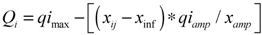
In a second step, a water quality index WQI model was proposed. A definition of quality measurement values (Qi) and aggregation weights (Wi) was established. Values of (Qi) were estimated based on each parameter value shown in Table 1.
Table 1. Parameters of limiting values for quality measurement (Qi) calculation.
QiEC (μScm−1)SARNaClHCO3
Meql−1
85–100200 ≤ EC < 750SAR < 32 ≤ Na < 3Cl < 41 ≤ HCO3 < 1.5
60–85750 ≤ EC < 1,5003≤ SAR < 63 ≤ Na < 64 ≤ Cl < 71.5 ≤ HCO3 < 4.5
35–601,500 ≤ EC < 3,0006≤ SAR < 126 ≤ Na < 97 ≤ Cl < 104.5 ≤ HCO3 < 8.5
0–35EC < 200 or SAR ≥ 12Na 2 < 2 or Cl ≥ 10HCO3 < 1 or
EC ≥ 3,000Na ≥ 9HCO3 ≥ 8.5
Note: The criteria established by [28].
Water quality parameters were represented by a non-dimensional number: the higher the value, the better the water quality. Values of Qi were calculated using the following equation, based on the tolerance limits shown in Table 1 and water quality results determined in the laboratory:
Water 04 00545 i003
where qimax is the maximum value of Qi for the class; xij is the observed value for the parameter; xinf is the value corresponding to the lower limit of the class to which the parameter belongs; qiamp is the class amplitude; xamp is the class amplitude to which the parameter belongs.
In order to evaluate xamp of the last class of each parameter, the upper limit was considered to be the highest value determined in the physical-chemical and chemical analysis of the water samples, then Wi values were normalized such that their sum equaled one.
Water 04 00545 i004
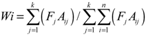
where Wi is the weight of the parameter for the WQI; F = component 1 autovalue; Aij is the explainability of parameter i by factor j; i is the number of physical- chemical and chemical parameters selected by the model, ranging from 1 to n; j is the number of factors selected in the model, varying from 1 to k.
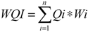
The water quality index was calculated by summation of Qi, and Wi values as:
Water 04 00545 i005
where WQI is a dimensionless parameter ranging from 0 to 100; Qi is the quality of the ith parameter, a number from 0 to 100, a function of its concentration or measurement; Wi is the normalized weight of the ith parameter, a function of its importance in explaining the global variability in water quality.
Division in classes based on the proposed water quality index, which was based on existent water quality indexes, and classes were defined considering the risk of salinity problems, soil water infiltration reduction, as well as toxicity to plants as observed in the classifications presented by [29]. Restrictions to water use classes were characterized as shown in Table 2.
Table 2. Water quality index characteristics.
WQIWater use restrictions
85 ≤ 100No restriction (Excellent)
70 ≤ 85Low restriction (Good)
55 ≤ 70Moderate restriction (Poor)
40 ≤ 55High restrictions (Very poor)
0 ≤ 40Severe restrictions (Unsuitable for irrigation)
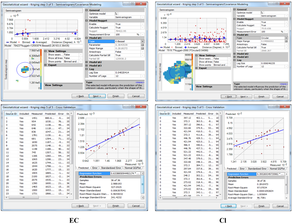
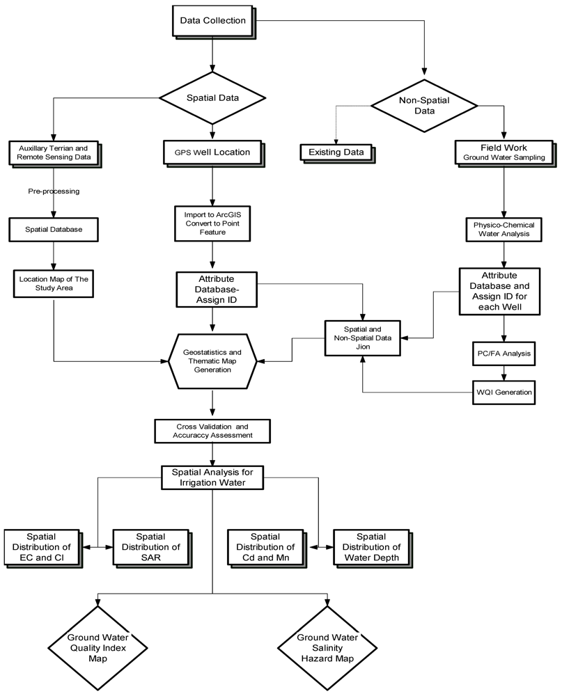
In a third step, the water quality data (attribute) was linked to the sampling location (spatial) in ArcGIS and maps showing spatial distribution were prepared to identify the variation in concentrations of the groundwater parameters at various locations of the study area. Different water quality maps were produced using point data like pH, EC, SAR, Cl, and B by ArcMap GIS software. Geostatistical analyses were performed using the Geostatistical analyst extension available in ESRI ArcMap (v. 10) [30]. Kriging differs from other methods (such as IDW), in which the weight function is no longer arbitrary, being calculated from the parameters of the fitted semivariogram model under the conditions of unbiasedness and minimized estimation variance for the interpolation. Thus, Kriging is regarded as best linear unbiased estimation (BLUE). A more detailed explanation of the method is given by [31,32,33,34,35]. Of the different Kriging techniques, the ordinary Kriging (OK) method was used in the present study because of its simplicity and prediction accuracy in comparison to other Kriging methods [31].
Geostatistical analysis was the first to fully explore the data in which the histogram, normality, trend of data, semivariogram cloud and cross covariance cloud of the raw data were observed [36]. Kriging methods work best if the data is approximately normally distributed [37]. Transformations were used to make the data normally distributed and satisfy the assumption of equal variability for the data. In ArcGIS Geostatistial Analyst, the histogram and normal QQPlots were used to see what transformations were needed to make the data more normally distributed. For each water quality parameter, an analysis trend was made. Directional influences (anisotropy) are critical to the accurate estimation of water quality surface. The directional search tool was used to remove the directional influences from the groundwater quality data. In this study, the semivariogram models were tested for each parameter data set. Prediction performances were assessed by cross validation. Cross validation allows determination of which model provides the best predictions. For a model that provides accurate predictions, the standardized mean error should be close to 0, the root-mean-square error and average standard error should be as small as possible (useful when comparing models), and the root-mean square standardized error should be close to 1 [37]. Finally, to produce a simple (salinity and WQI) hazard map, simple classes were used. The suitability map obtained from the computed index value was evaluated according to three categories: unsuitable (0–40), moderate (40–70), and suitable (70–100). Also the salinity hazard map was assessed based on three categories: unsuitable (˃1500 μScm−1), moderate (1500–750 μScm−1), and suitable (˂750 μScm−1). The area with WQI value of less than 40 was considered to be poor quality irrigation water not suitable for irrigating agricultural fields. Such water could impair soil quality and result in yield loss. As a rule of thumb, water extraction from such areas should be avoided.

3. Results and Discussion

3.1. Overall Statistical Analysis and Evaluation

Table 3 shows the summary of the statistical evaluation of the laboratory analyses conducted on the samples. 15 of 20 parameters were used in the analysis at this stage because the remaining five parameters were used in the calculation of SAR and RSC parameters. The pH of the water samples was within a range of 7–8. The overall EC values varied between 642 and 2686 μScm−1. EC was lowest for a sample collected from Village 1 (Sample 3) while the highest occurred in a sample from Village 4 (Sample 32). The chloride concentration of the water samples was within a wide range of 124.1–570.9 ppm. The concentration of chloride in most of the areas was high with the maximum of 570.86 ppm in Village 2 (Sample 9). The range of SAR values in the water samples was 1.83–8.47, where the highest SAR value related to Village 4 (Sample 32) and the lowest value related to Village 1 (Sample 3). Based on the RSC criterion, all water samples were −7.1 to −1.86 (Table 3). Water samples analyses revealed that heavy metal pollution of groundwater was low. The variations in the distribution of the investigated heavy metals (Cu, Fe, Pb, Mn, Ni and Zn) in the study area were small. Except for Cd whose concentration in the water samples was detected to be abnormally high (0.013 ppm) and above the standard value (0.01ppm) for irrigation [38,39], all other heavy metals were within the maximum permissible range (Table 3).
Table 3. Descriptive statistics of water quality parameters of water samples.
ParametersRangeMinimumMaximumSumMeanSDSkewnessKurtosis
Depth to well316.00214.00530.0013,792.00383.11107.28−0.42−1.43
Elevation83.0082.00165.004,747.00131.8625.12−0.67−0.99
EC2,044.00642.002,686.0059,645.001,656.81540.32−0.46−0.59
pH1.146.998.13271.557.540.310.01−0.70
SAR6.641.838.47198.285.511.82−0.60−0.54
RSC5.24−7.10−1.86−145.52−4.041.56−0.26−1.04
Cl446.76124.10570.8612,385.18344.03115.68−0.24−0.62
B0.170.020.183.340.090.05−0.47−1.34
Fe0.190.000.192.600.070.060.72−0.21
Mn0.270.000.271.350.040.062.255.40
Cu0.120.000.121.370.040.030.49−0.32
Zn0.070.000.071.340.040.02−0.10−0.42
Cd0.0130.000.0130.070.0020.0032.345.62
Pb0.240.000.242.620.070.070.78−0.06
Ni0.170.000.170.580.020.042.657.53
All units except pH, SAR, RSC and EC are in ppm, Depth to well and Elevation, m; SD = Std. Deviation.
The only abnormal and interesting result of a higher Cd amount than the standard value in groundwater at the depth varied between 214 and 530 m. The reason for the existence of Cd in Darb El-Arbaein is that cadmium can be present in groundwater through contact with soluble rocks and minerals. The primary mineral associations of cadmium are with otavite (CdCO3), greenockite (CdS). Soil weathering can lead to the release of the Cd2+ ions, which are generally soluble and mobile in water. Other sources of cadmium in groundwater include mining (sulfide ores of zinc), industrial operations, burning of fossil fuels, and fertilizer application. An important source of cadmium is the production of phosphate. Phosphate deposits were recorded at a depth of 600m in the Darb El Arbaein area [40]. Substitution of cadmium with natural apatite has also been documented [41] and may be a more common route for partitioning to phosphate minerals at concentrations undersaturated with respect to precipitation of cadmium phosphate. Cadmium is known to form solid solutions with calcium carbonate (calcite) [42,43,44].

3.2. Principal Component and Factorial Model

Table 4 shows the correlation matrix for the analyzed parameters. High correlations (above 0.9) were observed between EC and SAR and Cl. Kaiser-Meyer-Olkin (KMO) adequacy test for coefficient magnitude comparison indicated an optimum value of 0.82, indicating that the factorial model may be applied without restrictions. A similar result was found by [45] in the water quality evaluation in tropical lake systems, with a KMO value of 0.85, considered adequate for the study.
Table 4. Correlation matrix for the analyzed parameters.
ParametersElevationDepth to WellECpHSARRSCClBFeMnCuZnCdPbNi
Elevation1--------------
Depth to Well0.8031-------------
EC0.6970.7251------------
pH0.5970.6010.4501-----------
SAR0.7610.7730.9550.4961----------
RSC−0.226−0.322−0.780−0.143−0.5941---------
Cl0.4780.4990.9400.3040.836−0.8831--------
B0.8950.8950.7170.6580.817−0.1990.4871-------
Fe0.4230.3200.1940.0890.158−0.1540.0420.2381------
Mn−0.589−0.628−0.670−0.256−0.6790.387−0.600−0.672−0.0091-----
Cu0.5590.6260.4320.2650.544−0.0260.2530.5830.102−0.2381----
Zn0.0670.1300.1580.0310.089−0.2760.0770.0060.5010.151−0.1611---
Cd−0.192−0.091−0.223−0.184−0.352−0.053−0.194−0.2470.178−0.028−0.4030.3411--
Pb0.2850.2580.2360.0560.298−0.0510.1380.2580.076−0.1670.1180.5100.1181-
Ni−0.155−0.0420.075−0.1520.034−0.2650.128−0.1620.3410.043−0.1610.2290.0990.2031
Table 5 shows the principal component analysis application to describe the dispersion of original parameters which implies a four component model, explaining 77.393% of total variance, diluted in fifteen dimensions. This result is in agreement with the works of [25,27,46] in which the two to three first generated components explain a great part of the variation of original data (60% to 90%). In many cases the use of these components allows the description of the entire data system without significant loss of information. Selection of this four-component model used the criterion described by [47] considering only those components with a variance that had an auto-value above one. Any component must explain a variance above that presented by a single variable. This criterion is observed by [48] upon water quality evaluation in the Guadalquivir river in the south of Spain, where through PC three hydrochemical factors were identified with variances above unity and explaining 79.1% of total variance of the data.
Table 5 presents factorial loads for the chemical and calculated parameters. A matrix rotation was performed and data for factorial loads and communalities after transformation are presented in Table 5. The first Factor explains 43.371% of total variance in the data, whereas the second and third factors explain 15.366% and 11.510%, respectively. In the first Factor/Component, parameters such as elevation, depth to well, EC, SAR, Cl, B and Mn present a load above 0.70, indicating the most common composition of the observed parameters. In the second Factor/Component, parameters Zn and Ni show high factorial loads of 0.774 and 0.625 respectively. The fourth Factor/Component showed Cd as the element with the load (0.644).
Table 5. Factorial loads for the observed parameters.
ParametersFactorial loads matrix
F1F2F3F4
EC0.96660.1866−0.13030.0068
pH0.5579−0.29830.0767−0.0226
SAR0.9710−0.0364−0.06360.0481
RSC−0.6320−0.69850.2836−0.0091
Cl0.83920.3776−0.3457−0.0165
Na0.97810.1065−0.05800.0474
Ca−0.78830.4831−0.3159−0.0163
Mg0.53950.5618−0.22830.0896
HCO30.8209−0.44690.2306−0.0632
Fe0.25290.23560.63480.3909
Mn−0.71490.07750.12270.4571
Cu0.5380−0.51130.03340.3242
Zn0.14420.51010.6947−0.0016
Cd−0.24840.42130.3839−0.6110
Pb0.28840.09290.5945−0.2261
Ni0.01790.53960.24580.4044
Variance %47.03015.51210.7256.017
Cumulative %47.03062.54173.26679.284
Extraction method: Principal component analysis.

3.3. WQI Development

In order to develop the proposed WQI, EC, Cl, Na, HCO3 and SAR parameters were used. These carry the major factorial load (above 0.82 in Table 5), that is, they best define water quality [46,47,48]. Only these parameters have reference, weight, and hazard ranges, however the other parameters are missing from in the literature. Henceforth, the weight of each parameter was based on the variance of the first factor (Table 6), associated with the explainability of each parameter, in relation to this factor. The normalized weights (Wi), computed through Equation (2), are listed in Table 6. The suitability index, which wascalculated based on Equation 3, is shown in Table 7.
Table 6. Weights for the Water Quality Index (WQI) parameters.
ParametersECSARNaClHCO3Total
Wi0.24120.24230.20940.24410.06301.000
Table 7. Groundwater Quality Index (WQI).
LocationSample No.WQIWater qualityLocationSample No.WQIWater quality
Village 1153.48Very poorVillage 3 1944.04Very poor
275.29Good2060.65Poor
375.21Good2154.92Very poor
474.16Good2253.37Very poor
581.98Good2348.42Very poor
Village 2649.13Very poor2445.53Very poor
788.60Excellent2545.84Very poor
850.71Very poor2644.75Very poor
947.93Very poorVillage 42743.88Very poor
1065.90Poor2840.64Very poor
1185.42Excellent2945.18Very poor
1268.42Poor3043.22Very poor
1370.40Good3141.40Very poor
Village 31451.14Very poor3238.87Unsuitable for irrigation
1545.38Very poor3350.86Very poor
1649.89Very poor3446.15Very poor
1746.01Very poor3546.31Very poor
1843.27Very poor3645.44Very poor
Table 7 shows the suitability index map calculated. The suitability index is calculated to determine the suitability of water for irrigation purposes. Suitability index values revealed that the groundwater in the study area is of “suitable” quality with the suitability index ranging from 85 to 100 (two wells are of excellent water quality) and therefore can be used for irrigation usage. Most of the samples are very poor (25 wells) with a suitability index range from 40 to 55. One sample (well No. 32) is of “unsuitable” quality and cannot be used for irrigation purposes. Five wells are of good quality and three wells of poor quality. Overall, most of Village 1 wells are of good quality and can be used for irrigation with low restrictions, except for well No. 1 which is of very poor quality. Village 2 wells are of very poor quality with high restrictions for irrigation except for wells No. 7,11 that are of excellent quality and can be used for irrigation with no restriction. The wells of villages 3,4 are of very poor quality and can be used for irrigation only with high restrictions.
Overall, the results in Table 7 indicate that villages 1,2 generally have good water quality, however villages 3,4 have a very poor water quality. Restrictions for using this water in irrigation at long term are required especially because the soil texture is heavy and the climate is hot.

3.4. Spatial and Interpolation Analysis of Groundwater Quality Variation

Water samples were taken from 36 wells in the study area. The data was checked by a histogram tool and normal QQPlots to see if it showed a normal distribution pattern. Normal QQPlots provide an indication of univariate normality. If the data is asymmetric (i.e., far from normal), the points will deviate from the line. Histogram and normal QQPlot analysis were applied for each water quality parameter. It was determined that electrical conductivity, chloride, Mn, Cd, Pb, Ni and SAR concentrations showed normal distributions, however, only the pH, B, and Zn parameters did not show normal distributions. For these parameters, a log transformation was applied to make the distribution closer to normal. For each water quality parameter, an analysis trend was made and it was determined that there was no global trend for all parameters. In this study, the semivariogram models (circular, spherical, tetraspherical, pentaspherical, exponential, gaussian, rational quadratic, hole effect, K-Bessel, J-Bessel, and stable) were tested for each parameter data set. Prediction performances were assessed by cross validation, which examines the accuracy of the generated surfaces.
Figure 3 and Table 8 list cross validation results of the examined validity of the fitting models and parameters of semivariograms for EC and Cl parameters. All of the water quality parameters were assessed by cross validation and given EC and Cl parameters as an example. For the EC sample, the standardized mean range is from 0.006153 to −0.000346 and the RMSS range is from 0.9642 to 0.9788. In this case, for the EC parameter the best fit is the J-Bessel model (SME −0.000346) and Circular model for Cl with a 0.005528 standardized mean error. It is closest to zero, and the 0.9788 RMSS value is closest to 1. When the average estimated prediction standard errors are close to the root-mean-square prediction errors from cross-validation, then you can be confident that the prediction standard errors are appropriate [37].
After applying different models for each water quality parameter examined in this study, the error was calculated using cross validation and models giving best results were determined. Table 9 shows the most suitable models and their prediction error values for each parameter. Table 9 also shows that for different parameters different models may give better results. For water quality parameters, RMSS range from 0.945 to 1.2452.
Table 8. Cross validation results of EC and Cl parameters.
ModelsPrediction errors
MeanRoot mean squareAverage standard errorMean standardizedRoot mean square standardized
ECClECClECClECClECCl
Circular (Cl)2.83110.2810331.71196.730343.97697.0700.005530.000010.96791.006
Spherical2.80750.5185331.25094.960343.47696.9000.005490.00240.96850.983
Tetraspherical2.78621.6871330.96595.270343.16896.9900.005440.0140.96840.985
Pentaspherical2.78411.0608330.81195.410343.00397.0490.005450.0130.96850.985
Exponential2.99111.5944328.13196.375341.10697.3270.006090.0130.96750.990
Gaussian−0.20961.7452324.44095.762334.37896.699−0.002680.01470.97720.992
Rational Quadratic2.47401.6371329.06896.402338.29497.6130.004780.0130.97720.989
Hole Effect−0.60051.5360322.29194.020332.47996.75−0.003500.0120.97750.970
K-Bessel2.92601.7198327.29995.911341.62196.7590.006150.0140.96420.990
J-Bessel (EC)0.62901.4001323.98293.697333.44696.973−0.000350.0110.97880.969
Stable2.98801.7452327.05295.762341.42396.6990.006300.01470.96430.992
Table 9. Fitted parameters of the variogram model for groundwater quality.
ParametersModelsPrediction Errors
MeanRoot mean squareAverage standard errorMean standardizedRoot mean square standardized
ECJ−Bessel0.6290323.98333.45−0.000340.9790
pH*Rational Quadratic0.00300.25800.25400.005841.0060
SARStable0.00581.06471.32800.003811.0647
ClCircular0.281097.07096.7380.000011.0057
B*Gaussian0.00150.01470.0254−0.045801.2452
Zn*Spherical−0.00020.01390.0143−0.021080.9825
MnStable0.000010.00880.0093−0.001400.9517
CdCircular−0.00050.01190.0107−0.027501.0930
PbStable−0.00210.07200.0760−0.026300.9450
NiSpherical−0.00000.03810.0396−0.002300.9640
* Logarithm is used to normalize data.
Table 10 shows parameters of water quality variograms. The ratio of nugget to sill variances, expressed as percentage, can be regarded as a criterion to classify the Spatial Dependency (Sp.D) of parameters. If the ratio is less than 0.25, the variance has strong spatial dependency and if the ratio ranges between 0.25 and 0.75, the variance has moderate spatial dependency. All parameters of water quality have a strong spatial structure except Cl (0.67). Also the effective ranges of most parameters are close together, within the range of 600 to 850 m.
Table 10. Spatial dependency (Sp.D) and range of the interpolated models for different parameters.
ParametersModelNugget/Sill ratio (Sp.D)Range (Km)
ECJ-Bessel0.030.60
ClCircular0.670.82
SARStable0.360.73
CdCircular0.230.85
MnStable0.120.65
Sp.D = Spatial Dependency
Figure 3. Cross validation and semivariograms model for EC and Cl parameters.
Water 04 00545 g003
Figure 4 shows the spatial distribution of different parameters (e.g., EC, pH, SAR, Cl…) in the study area and some selected parameters (e.g., Cd, Mn, and water depth), which have F1 and F4 factorial loads. The groundwater quality prediction maps show the concentration distribution generated from the surface map developed from the cross validation process.
Figure 4. Spatial distributions of EC, SAR, Cl, Cd, Mn and water depth.
Water 04 00545 g004

3.5. Well Water Quality Mapping for Agricultural Purposes

The groundwater quality maps for agricultural purposes are shown in Figure 5.
Figure 5. Groundwater salinity hazard map and WQI map of Darb El-Arbaein.
Water 04 00545 g005
The whole area is divided into three classes on the basis of EC. The water quality for irrigation purposes depends on the salinity classified into suitable, moderate, and unsuitable. Also, the map of WQI is presented. When the computed index value is bigger than 70, the area is considered to have minimum problems with respect to irrigation quality. Therefore, a well drilled in this zone is considered to represent ideal conditions for irrigation water quality. When the computed index value is between 40 and 70, the water demonstrates moderate suitability for irrigation purposes. On the other hand, values below 40 indicate water that should only be used with caution and better be avoided, particularly for sensitive crops. Three of the groundwater samples fall into the moderate WQI. Most of the samples (26) fall into the unsuitable WQI category. Seven samples fall into the suitable WQI category. Groundwater samples that fall into the low salinity hazard class and high WQI can be used in irrigation for most crops and the majority of soils.
The map of villages 3,4 (Figure 5) shows that 382.35 ha (10.09%) of area fall into the moderate category, however, much of the area (3407.38 ha) has unsuitable water quality. For the villages 1,2, the corresponding area of suitable category is 266.66 ha (13.79%), however, the moderate category is 1666.79 ha. The observed low suitability index of the groundwater quality is due to the desert location and the deficiency of water and rainfall, which leads to the need to dig deep and semi-deep wells. Since the map shows the spatial distribution of irrigation water quality in the area as index values, it is now much easier for a decision maker to assess the quality of water for irrigation purposes and further locate the most suitable site for drilling wells to extract irrigation water.
Groundwater resource degradation is an issue of significant societal and environmental concern in the Darb El-Arbaein area. In order to prevent groundwater pollution and avoid the future need for costly remediation efforts, GIS can be used to assess groundwater pollution. It is also helpful for the public to understand that the quality of water is a useful tool in many ways in the field of water quality management [49].

4. Conclusions and Future Outlook

The present paper proposes a simple model to assess and map groundwater suitability for irrigation purposes in the Darb El-Arbaein area. Factor/Principal Component Analysis permitted the description of parameters involved in the processes that define water quality in the Darb El-Arbaein through a four-component model, the components of which explain 79.28% of total data variance, previously diluted into thirteen dimensions. The ordinary Kriging method was used for the preparation of thematic maps of groundwater quality parameters such as electrical conductivity, sodium adsorption ratio, chloride, and heavy metals. The circular semivariogram model was best fitted for chloride and Cd parameters where the spherical model fitted best for Ni and Zn parameters. The stable semivariogram model best fitted Pb and SAR parameters where the J-Bessel model fitted best for the EC parameter. High salinity was due to the high chloride concentration in the groundwater. The map of villages 1,2 indicates the presence of about 13.79% of the study area which contains suitable groundwater for irrigation. However, in villages 3,4, 10.09% of the area falls into the moderate category for irrigation purposes. The groundwater quality index was devised to analyze the combined impact of different quality parameters on irrigation purposes. The Water Quality Index (WQI) developed and proposed in this study provides an easy-to-use tool that could help analyze the overall quality of irrigation water. Overall, the proposed index incorporates the EC parameter to represent salinity limitation; SAR and EC to represent permeability limitation; sodium, chloride, boron and trace elements to represent specific ion toxicity, HCO3 and pH to represent effects on sensitive crops.
The application of WQI in this study has been found useful in assessing the overall quality of water. It is also helpful for the public to understand that the water quality is a useful tool in many ways in the field of water quality management. The WQI used provides a non-expert with an easy way of understanding the overall water quality. The present study demonstrates high efficiency for GIS to analyze complex spatial data. The GIS would help to apply the groundwater management practices such as proper groundwater resource management in terms of groundwater quality and quantity. Groundwater quality maps produced as a result of this research should be taken into account by decision-makers for sustainable land-use management in Darb El-Arbaein.
An analysis of the nature and types of land-use and its associated impact on groundwater quality is essential for a proper understanding of the present environmental problems and linking groundwater quality and land-use. The relationship between land-use and water quality is bidirectional. Land-use activities have direct impacts on water quality, while water quality greatly influences the siting of land-use activities. Inappropriate land-use, particularly poor land management, causes chronic groundwater quality problems. Acute groundwater quality problems are common and arise from unsuitable land use. There remains a lack of coherent land-use plans that protect and improve water quality. None of the research has advocated an overall spatial planning approach and the widespread restructuring of land-use, which we believe are needed to get to grips with the conflicts between groundwater and land-use. There is a real necessity to tackle these problems. So, further research could be to answer the following question: What are the effects of groundwater quality on land-use? One cannot discuss the future impact of land-use on groundwater without considering the scale used. So, further research also should answer the question: “Does scale matter?” The purpose is to evaluate the use of different spatial and temporal resolution satellite images for delineating meaningful land-use change information to support database development at different scales.

References

  1. Hu, K.; Huang, Y.; Li, H.; Li, B.; Chen, D.; White, R.E. Spatial variability of shallow groundwater level, electrical conductivity and nitrate concentration, and risk assessment of nitrate contamination in North China Plain. Environ. Int. 2005, 31, 896. [Google Scholar] [CrossRef]
  2. Asadi, S.S.; Vuppala, P.; Anji, R.M. Remote sensing and GIS techniques for evaluation of groundwater quality in municipal corporation of Hyderabad (Zone-V), India. Int. J. Environ. Res. Public Health 2007, 4, 45–52. [Google Scholar] [CrossRef]
  3. Lado, L.R.; Polya, D.; Winkel, L.; Berg, M.; Hegan, A. Modelling arsenic hazard in Cambodia: A geostatistical approach using ancillary data. Appl. Geochem. 2008, 23, 3010. [Google Scholar] [CrossRef]
  4. Buchanan, S.; Triantafilis, J. Mapping water table depth using geophysical and environmental variables. Groundwater 2009, 47, 80. [Google Scholar] [CrossRef]
  5. Horton, R.K. An index number system for rating water quality. J. Water Pollut. Control Fed. 1965, 37, 300–305. [Google Scholar]
  6. Shihab, A.S.; Al-Rawi, S.M. Application of water quality index to Tigris River within Mosul city. Rafidain J. Sci. 1994, 4, 80–92. [Google Scholar]
  7. Al-Hussain, M.H. Establishment WQI for Tigris River within Mosul City. M.Sc. Thesis, University of Mosul, Mosul, Iraq, 1998. [Google Scholar]
  8. Debels, P.; Figueroa, R.; Urrutia, R.; Barra, R.; Niell, X. Evaluation of water quality in the Chillan River (Central Chile) using physicochemical parameters and a modified water quality index. Environ. Monit. Assess. 2005, 110, 301–322. [Google Scholar] [CrossRef]
  9. Numaan, M.M. Development of Water Quality Index for Tigris River Water Between Alsharqat and Alboajeel. M.Sc. Thesis, University of Tikrit, Tikrit, Iraq, 2008. [Google Scholar]
  10. Bhatti, M.T.; Latif, M. Assessment of water quality of a River using an indexing approach during the low-flow season. J. Irrig. Drain. 2009, 60, 103–114. [Google Scholar] [CrossRef]
  11. Fulazzaky, M.A. Water quality evaluation system to assess the status and the suitability of the Citarum river water to different uses. J. Environ. Monit. Assess. 2009, 168, 669–684. [Google Scholar] [CrossRef]
  12. Meireles, A.C.M.; de Andrade, E.M.; Chaves, L.C.G.; Frischkorn, H.; Crisostomo, L.A. A new proposal of the classification of irrigation water. Rev. Cienc. Agron. 2010, 41, 349–357. [Google Scholar] [CrossRef]
  13. Orebiyi, E.O.; Awomeso, J.A.; Idowu, O.A.; Martins, O.; Oguntoke, O. Assessment of pollution hazards of shallow well water in Abeokuta and environs, Southwest Nigeria. Am. J. Environ. Sci. 2010, 6, 50–56. [Google Scholar] [CrossRef]
  14. He, J.Y.; Jia, X. ArcGIS geostatistical analyst application in assessment of MTBE contamination. In Proceedings of ESRI User Conference 2004, Fremont, CA, USA, 9 August 2004; Available online: http://gis.esri.com/library/userconf/proc04/docs/pap1628.pdf (accessed on 10 July 2012).
  15. Kumar, A.; Maroju, S.; Bhat, A. Application of ArcGIS Geostatistical Analyst for interpolating environmental data from observations. Environ. Prog. 2007, 26, 220–225. [Google Scholar] [CrossRef]
  16. Woo, K.W.; Jo, J.H.; Basu, P.K.; Ahn, J.S. Stres intensity factor by p-adaptive refinement based on ordinary Kriging interpolation. Finite Elem. Anal. Des. 2009, 45, 227–234. [Google Scholar] [CrossRef]
  17. Liu, X.; Wu, J.; Xu, J. Characterizing the risk assessment of heavy metals and sampling uncertainty analysis in paddy field by geostatistics and GIS. Environ. Pollut. 2005, 141, 257–264. [Google Scholar]
  18. Pozdnyakova, L.; Zhang, R. Geostatistical analyses of soil salinity in a large field. Precis. Agric. 1999, 1, 153–165. [Google Scholar] [CrossRef]
  19. Ramakrishnaiah, C.R.; Adashiv, C.; Ranganna, G. Assessment of water quality index for the groundwater in Tumkur Taluk, Karnataka State, India. E J. Chem. 2009, 6, 523–530. [Google Scholar] [CrossRef]
  20. Arsalan, M.H. A GIS Appraisal of Heavy Metals Concentration in Soil; Technical Report for American Society of Civil Engineers: New York, NY, USA, 2004. [Google Scholar]
  21. Karanjac, J. Regional Programme for the Development and Utilization of the Nubian Sandstone Aquifer; Technical Report for Centre for Environment & Development for the Arab Region & Europe: Cairo, Egypt, 1995. [Google Scholar]
  22. Said, R. The Geology of Egypt; American Elsevier Pub. Co.: NewYork, NY, USA, 1962. [Google Scholar]
  23. American Public Health Association, Standard Methods for the Examination of Water and Wastewater, 20th edAmerican Public Health Association: Washington, DC, USA, 1998.
  24. Hair, J.F.; Black, W.C.; Babin, B.J.; Anderson, R.E.; Tatham, R.L. Multivariate Data Analysis, 6th ed; Pearson Prentice Hall: Upper Saddle River, NJ, USA, 2005. [Google Scholar]
  25. Simeonov, V.; Stratis, J.A.; Samara, C.; Zachariadis, G.; Voutsa, D.; Anthemidis, A.; Sofoniou, M.; Kouimtzis, T. Assessment of the surface water quality in Northern Greece. Water Res. 2003, 37, 4119–4124. [Google Scholar] [CrossRef]
  26. Wunderlin, D.A.; Dıaz, M.P.; Ame, M.V.; Pesce, S.F.; Hued, A.C.; Bistoni, M.A. Pattern recognition techniques for the evaluation of spatial and temporal variations in water quality—A case study: Suquia river basin (Cordoba-Argentina). Water Res. 2001, 35, 2881–2894. [Google Scholar] [CrossRef]
  27. Helena, B.; Pardo, R.; Vega, M. Temporal evolution of groundwater composition in an alluvial aquifer (Pisuerga river, Spain) by principal component analysis. Water Res. 2000, 34, 807–816. [Google Scholar] [CrossRef]
  28. Ayers, R.S.; Westcot, D.W. A Qualidade da Água na Agricultura (in Portuguese), 2nd ed; UFPB Universidade Federal da Paraíba: João Pessoa, Brazil, 1999; p. 218. [Google Scholar]
  29. Bernardo, S. Manual of Irrigation, 4th ed; Universidade Federal de Viçosa: Vicosa, Brazil, 1995; p. 488. [Google Scholar]
  30. ESRI, ArcMap Version 10 User Manual; ESRI: Redlands, CA, USA, 2011.
  31. Isaaks, E.H.; Srivastava, R.M. An Introduction to Applied Geostatistics; Oxford University Press: New York, NY, USA, 1989. [Google Scholar]
  32. Stein, M.L. Interpolation of Spatial Data: Some Theory for Kriging; Springer: Berlin, Germany, 1999. [Google Scholar]
  33. Yamamoto, J.K. An alternative measure of the reliability of ordinary Kriging estimates. Math. Geol. 2000, 32, 489–509. [Google Scholar] [CrossRef]
  34. Gringarten, E.; Deutsch, C.V. Teacher’s aide variogram interpretation and modeling. Math. Geol. 2001, 33, 507–534. [Google Scholar] [CrossRef]
  35. Omran, E.S.E. Improving the prediction accuracy of soil mapping through Geostatistics. Int. J. Geosci. 2012, in press. [Google Scholar]
  36. Sarangi, A.; Cox, C.A.; Madramootoo, C.A. Geostatistical methods for prediction of spatial variability of rainfall in a mountainous region. Trans. ASAE 2005, 48, 943–954. [Google Scholar]
  37. Johnston, K.; Hoef, J.M.V.; Krivoruchko, K.; Lucas, N. Using ArcGIS Geostatistical Analyst; ESRI: Redlands, CA, USA, 2001. [Google Scholar]
  38. World Health Organization, Guidelines for Drinking Water Quality, 2nd ed; World Health Organization: Geneva, Switzerland, 1993; Volume 1.
  39. FAO, Water Quality for Agriculture; FAO: Rome, Italy, 1985.
  40. Said, R. The Geology of Egypt; Taylor & Francis: New York, NY, USA, 1990. [Google Scholar]
  41. Sery, A.; Manceau, A.; Greaves, G.N. Chemical state of Cd in apatite phosphate ores as determined by EXAFS spectroscopy. Am. Mineral. 1996, 81, 864–873. [Google Scholar]
  42. Tesoriero, A.J.; Pankow, J.F. Solid solution partitioning of Sr2, Ba2, and Cd2 to calcite. Geochim. Cosmochim. Acta 1996, 60, 1053–1063. [Google Scholar] [CrossRef]
  43. Chiarello, R.P.; Sturchio, N.C.; Grace, J.D.; Geissbuhler, P.; Sorensen, L.B.; Cheng, L.; Xu, S. Otavite-calcite solid-solution formation at the calcite-water interface studied in situ by synchrotron X-ray scattering. Geochim. Cosmochim. Acta 1997, 61, 1467–1474. [Google Scholar]
  44. Martin-Garin, A.; van Cappellen, P.; Charlet, L. Aqueous cadmium uptake by calcite: A stirred flow-through reactor study. Geochimi.Cosmochim. Acta 2003, 67, 2763–2774. [Google Scholar] [CrossRef]
  45. Parinet, A.L.; Legube, B. Principal component analysis: An appropriate tool for water quality evaluation and management—Application to a tropical lake system. Ecol. Model. 2004, 178, 295–311. [Google Scholar] [CrossRef]
  46. Prado, R.M.; Fernandes, F.M.; Natale, W. Lime and slag evaluated by leaf analysis, macronutrient accumulation and export of sugarcane. Sci. Agric. 2002, 59, 129–135. [Google Scholar] [CrossRef]
  47. Norusis, M.J. SPSS Base System User’s Guide; SPSS Inc.: Chicago, MI, USA, 1990; p. 520. [Google Scholar]
  48. Mendiguchia, C.; Moreno, C.; Galindo-Riaño, M.D.; García-Vargas, M. Using chemometric tools to assess anthropogenic effects in river water—A case study: Guadalquivir River (Spain). Anal. Chím. Acta 2004, 515, 143–149. [Google Scholar]
  49. Yisa, J.; Jimoh, T. Analytical studies on water quality index of river landzu. Am. J. Appl. Sci. 2010, 7, 453–458. [Google Scholar] [CrossRef]

