Abstract
We examine in some detail the interaction of water molecules with the radiative electromagnetic field and find the existence of phase transitions from the vapor phase to a condensed phase where all molecules oscillate in unison, in tune with a self-trapped electromagnetic field within extended mesoscopic space regions (Coherence Domains). The properties of such a condensed phase are examined and found to be compatible with the phenomenological properties of liquid water. In particular, the observed value of critical density is calculated with good accuracy.
1. Introduction
In the last two decades a conceptual change has occurred in the physics of condensed matter. For a long time condensed matter has been conceived as an ensemble of atoms/molecules kept together by static short-range forces. Liquid water has been no exception to this trend. In references [1,2] much material has been presented to describe the formation of a network of water molecules tied by the bindings named H-bonds, which should emerge from highly directional protuberances protruding from the molecule electron clouds. However, a conceptual difficulty emerges here, since, in order to fit experimental data [3], H-bonds should be conceived as short-lived; the lifetime varies with temperature from 20 ps at 250 K to 2 ps at 300 K. How is it possible to treat in a static approximation an electric charge structure (the H-bond) which lives so short a time? An electromagnetic (EM) field having at least the same time of oscillation should be necessarily introduced. Therefore the physical system of water molecules tied together would demand necessarily, in the framework of present knowledge, the explicit consideration of the interaction between water molecules and a radiative EM field. However when this problem is addressed in the theoretical framework of Quantum Electrodynamics (QED), a configuration of the system molecules + field emerges different from the usual network of molecules kept together by forces. In the new configuration, molecules oscillate in unison between two single-particle states, in tune with a non-vanishing EM field trapped in the ensemble of molecules. In this new state, termed coherent, the relevant physical variable is phase φ. QED connects φ to the EM potentials through the equations (in SI units)

In the above equation, Ā is the magnetic vector potential, V is the electric potential, h is Planck’s constant and e is the electron electric charge. Consequently, the phase correlations within the ensemble of coherent molecules are kept not by the EM fields but by their potentials, which, by the way, propagate in space at the phase velocity, which, as is well-known, could be larger than c. In Reference [4] a detailed mathematical theory, based on QED, is presented, discussing the appearance of coherent solutions in the system water molecules + electromagnetic field, which give rise to the liquid.
On the other hand, the presence of coherence in nature has been recently revealed within living organisms. For instance, an article [5] appeared in Nature showing that within photosynthetic systems molecules are “wired together” in a coherent way. We quote verbatim from the abstract of Reference [5]:
“Intriguingly, recent work has documented that light-absorbing molecules in some photosynthetic proteins capture and transfer energy according to quantum-mechanical probability laws instead of classical laws at temperatures up to 180 K. This contrasts with the long-held view that long-range quantum coherence between molecules cannot be sustained in complex biological systems, even at low temperatures. Here, we present two-dimensional photon echo spectroscopy measurements on two evolutionarily-related light harvesting proteins isolated from marine cryptophyte algae, which reveal exceptionally long-lasting excitation oscillations with distinct correlations and anti-correlations, even at ambient temperature. These observations provide compelling evidence for quantum coherent sharing of electronic excitation across the 5-nm-wide proteins under biologically relevant conditions, suggesting that distant molecules within the photosynthetic proteins are ‘wired’ together by quantum coherence for more efficient light-harvesting in cryptophyte marine algae.”
Therefore, coherent correlations span at least 5 nm. The correlated molecules, as all biomolecules, are of course immersed in water, which accounts for the large majority (70% of mass and 99% of molar concentration) of the components of living organisms. Therefore, the coherent correlations among biomolecules should be propagated by water. However, G. Scholes et al. [6] produced a study, based on Molecular Dynamics, showing that EM correlations within a liquid obeying the assumptions usually made for water, fall off within a distance smaller than 2 nm. Consequently, we should conclude that the usual picture of liquid water is unable to account for the observations of the coherent structure of living organisms.
Additional evidence of the fact that biomolecules are phase-correlated is provided by thermodynamics. The Second Law of Thermodynamics prescribes that the yield η = W/Q of a thermal engine, where Q is the heat absorbed at the temperature T and W is the performed work, should not exceed the quantity ∆T/T where ∆T is the temperature decrease of the energy flow within the engine. In a typical living organism at room temperature η cannot exceed a few percent, whereas bio-electrochemical evidence of the membrane processes gives a value of about 70% [7]. To avoid a thermodynamic inconsistency, we are forced to conclude that a living organism is not a thermal engine, so that its component molecules are not independent but are phase-correlated; actually, the ensemble of coherent molecules is able to receive energy as free energy, since its entropy is vanishing. The above statement is corroborated by the result quoted in the literature [8] that a muscle is not a thermal engine but a quantum machine. In conclusion, we should accept that liquid water, at least within living organisms, should exist in a coherent state, supporting the suggestion coming from QED analysis.
In the following we will present a description of the QED results in more physical terms than in Reference [4], giving a physical intuition of the process of the emergence of coherence. The role of water coherence in biological organisms has been discussed in Reference [9].
2. Emergence of Coherence
In this section we will try to provide a physical intuition of the emergence of coherence within a composite quantum system, such as an ensemble of atoms/molecules. According to first principles, a quantum system (either particle or field) cannot but fluctuate; in particular vacuum also fluctuates, as shown by the phenomenon of the Lamb shift of the energy levels of hydrogen atoms. These levels exhibit energy values slightly below (about 1 ppm) the ones calculated by quantum mechanics, which is based on the assumption that the Coulomb field that connects the proton and the electron is classical (non-fluctuating). The above difference between measured and calculated values of the hydrogen energy levels, first detected by Lamb in 1947 [10], is the evidence that actually a fluctuating field should be present, just the one produced by the quantum fluctuations of the vacuum oscillators. Therefore, according to quantum physics, we should always assume that molecules are coupled to a quantized EM field.
In order to give to the reader a qualitative understanding of the origin of the collective interaction among molecules induced by their interaction with the EM field, we give a simple scale argument. The size of a molecule is about a few Angstroms (Å); in the case of water slightly more than 1 Å. The typical energy difference Eexc between two levels of an atom/molecule is in the order of some eV (say 10 eV); the photon supplying this energy could be extracted from the environment, at the very least from the quantum fluctuations of the vacuum, and its size (we mean by size the extent of the region where the photon can be located) is of course its wavelength λ = hc/Eexc which for Eexc = 10 eV gives λ = 1200 Å. We find, therefore, the surprising result that the tool able to change the internal structure of the molecule is about one thousand times more extended than the molecule itself. At the usual densities of gases on Earth (in the case of water vapor at the boiling point 2 × 10¹⁹ molecules∙cm3) one single photon able to affect the molecular structure would include within its own volume some 20,000 molecules! Hence the collectivizing feature of the interaction between molecules and EM fields.
Let us describe now how this process of interaction could occur. A fluctuation of the EM mode having the frequency corresponding to the energy jump among molecule levels emerges either from the quantum vacuum or from the thermal bath. This fluctuation involves simultaneously all the molecules present in the volume λ3 spanned by its wavelength λ, in the case of water some 20,000 molecules, as candidates to be excited. It excites one of them with a probability P which can be calculated from the Lamb shift. The molecule remains excited for a time tdecay (the decay time of the excited level) and then decays giving back the EM fluctuation, which could fly away or excite a second molecule. The probability PN that this fluctuation would give rise to an excitation of one out of the N molecules present within the ensemble would be, of course:
When this number is smaller than 1, the EM fluctuation would disappear eventually in the original background, but when the density reaches the critical value (N/V)crit such that:
The EM field loses the chance of leaving the ensemble of molecules and gets permanently trapped within the region, bouncing from one molecule to another. In a short time more photons undergo the same fate until a sizeable EM field grows in this region that will be called from now a Coherence Domain (CD) attracting from the environment other molecules of the same species that are, by definition, able to resonate with the growing EM field. In this way the system self-produces a negative pressure which counteracts the positive pressure of the vapor. An attractive dynamic arises which binds molecules together, giving rise to a large increase of the molecular density and of the EM field until a value of the molecular density is reached, where, as we will see in detail in the following, the trapped EM field grows exponentially (runaway) inducing a further increase of density. This runaway brings the density of the system to a limiting value given by the intermolecular distance at which the repulsive forces produced by the molecule hard cores come into play. The final result is a closely packed ensemble of molecules oscillating in phase with an EM field. This field is trapped within the CD since its oscillation time is renormalized by the interaction with molecules; the time of oscillation of the free photon should be actually supplemented by the time spent within the molecules in the form of excitation energy. Consequently, the frequency of the fields (matter and EM) in the CD, νCD, becomes smaller than the frequency ν0 of the free field and the squared mass of the photon, m2, becomes, according to the Einstein equation:
since we know that the mass of a free photon is zero. On the contrary, the above equation tells us that the mass of the photon oscillating in the CD becomes imaginary; therefore this photon is no longer a particle, is unable to propagate and gets trapped in the CD in form of a cohesion energy, not static but at the origin of the coherent oscillation of molecules. The outcome of the above complex multi-step dynamics is the actual spontaneous formation of a cavity for the EM field.
Let us address now the problem of the selection of one specific level in the above lasing dynamics in the case of multi-level molecules, as is the case of water molecules. Phenomenological evidence gives us the indication that the transition vapor-liquid occurs basically in two steps. In a first step, molecule condensation occurs at several points simultaneously giving rise to a slow growth of density; this step takes almost the whole time of transition, until a threshold is reached where very fast condensation dynamics takes place, bringing the system to the final liquid phase.
In the framework of the present quantum field theory approach, the process can be described as follows. Each molecular level is able a priori to give rise to a condensed phase based on the coherent oscillation of all molecules between the molecular ground state and the given excited level. For each molecular level this process implies a specific time of growth of the matter density and of the associated cavity. The level able to produce the highest negative pressure through the above dynamics would give rise to the dominant condensation, ruling out all the other molecular levels. A cavity having the size of the wavelength of the winner EM mode, which resonates with the excitation energy of the level, is therefore self-produced. When, as we will see in next section, the molecular density reaches the critical density for runaway, the second part of the transition takes place until the system settles in the final coherent configuration.
3. Mathematical Derivation of Coherence
Let us now rephrase the above argument in mathematical terms. In Reference [11], the general Lagrangian description of the interaction between an ensemble of N microscopic units and the EM field has been written down and the corresponding Euler-Lagrange equations of motion have been derived. In the present article we will start just from these equations, where the variables are the matter-field Ψ that describes the space-time distribution of molecules among the different individual molecular states and the EM field  .
.
. The mathematical description of the dynamics sketched in the above section is extremely complex when addressed in the case of multi-level molecules. Since this process is intrinsically a dispersive one, it is conceivable, as discussed in [12,13], that one should drop the usual rotating wave approximation (RWA) in the equations in order to get, as suggested in the abstract in [13], the irreversible time evolution of the system into a generalized coherent state, exhibiting entanglement of the modes in which the counter-rotating terms are expressed. We will do this in a future publication. In this paper we will omit the description of the process of selection of the winner mode and adopt the procedure of choosing the level according to the best-fit of the phenomenological consequences.
Let us address now the problem of the mathematical description of runaway. Since we are interested in the investigation of the onset of the coherent oscillation between two specific molecule levels, we limit ourselves to the consideration of the two-component matter-field describing the space-time distribution of molecules between the two levels. The contribution to the dynamics of the remaining levels will come into play via second-order radiative corrections and will be taken into account in due course. Moreover, since we expect that the outcome of this mathematical treatment will be the emergence of a coherent state where the molecule radiative dipoles  connecting the two levels are all aligned, we limit ourselves to consider only the component of the EM field A parallel to this common radiative dipole. Finally, for normalization reasons we introduce the reduced fields obtained by dividing the original fields by
  , so that we will reason on a per-molecule basis. Notice that in the following we will use the standard unit system of field theorists, namely the Natural Unit System where the Planck constant h, the speed of light c and the elementary charge e are without dimension and assume the values 2π, 1 and 0.302814 (Lorentz-Heaviside units) respectively. Consequently the energy difference ∆E = Eq − E0 = hωq/2π can be written simply as ωq; in the natural unit system energy and frequency have the same dimension as well as space and time. Energy therefore assumes the dimension of the inverse of a length. In this unit system 1 eV is equal to 50,677 cm−1.
connecting the two levels are all aligned, we limit ourselves to consider only the component of the EM field A parallel to this common radiative dipole. Finally, for normalization reasons we introduce the reduced fields obtained by dividing the original fields by , so that we will reason on a per-molecule basis. Notice that in the following we will use the standard unit system of field theorists, namely the Natural Unit System where the Planck constant h, the speed of light c and the elementary charge e are without dimension and assume the values 2π, 1 and 0.302814 (Lorentz-Heaviside units) respectively. Consequently the energy difference ∆E = Eq − E0 = hωq/2π can be written simply as ωq; in the natural unit system energy and frequency have the same dimension as well as space and time. Energy therefore assumes the dimension of the inverse of a length. In this unit system 1 eV is equal to 50,677 cm−1.Moreover we introduce the adimensional time τ = ωq·t and factor out the term exp(−iτ) from all the fields. We define therefore the following reduced field:
where χ0 is the field describing the molecules in the ground state |0> and χq describes the molecules in the excited state |q>.
Three equations of motion, named coherence equation (CE), arise from the general formalism of QED [11] using the rotating wave approximation (RWA). The first equation corresponds to a process where matter in the excited state χq de-excites and reaches the ground state χ0, releasing an EM field A. The second equation describes a process where matter in the ground state χ0 is shifted to the excited state χq by the absorption of the EM mode described by A. The amplitude of the above processes is governed by the coherent coupling constant:
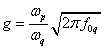
between the matter field and the EM field, where:

is the electron plasma frequency and f0q is the oscillator strength [14] of the optical transition between the states |0> and |q>. By neglecting the spatial dependence, the first two coherence equations are:
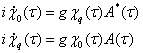
where the dot over the symbols indicates the derivative with respect to the adimensional time τ; the photons being described by the field A if absorbed and by the field A* if emitted. Now, by multiplying the first equation by χ0* and the second one by χq* and by adding them together with their conjugates, it is possible to derive the conservation relationship:

meaning that the number of molecules is conserved.
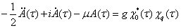
The third equation of the CE describes the evolution of the EM field which receives three contributions. The first contribution comes from the direct transitions governed by the constant g between the two levels. The second contribution comes from the two-step transitions (named dispersive transitions) governed by the constant µ, called photon mass term, where matter makes a first jump from the ground state to an intermediate virtual state |n> (n ≠ q) and a second jump from the latter to the final state. The third contribution is given by the vacuum through the so-called gauge properties of the EM field. The name for the coupling constant µ is connected to the fact, mentioned above, that the EM field acquires an imaginary mass because of the increased oscillation time (and consequently of the reduced frequency) of the field when tightly coupled with molecules that continuously emit and reabsorb the photons that compose the coherent EM field. In mathematical terms, the third coherence equation may be written:
Moreover, we are able to show the existence of two conserved quantities, Q and H. It is very easy to check that the quantity

is a conserved quantity. Actually, if we differentiate Equation (8) with respect to τ and replace the derivatives with the values given by the CE we get zero. Similarly the quantity

can also be shown to be conserved. In Reference [11], Q has been identified with the momentum per particle and H with total energy per particle. Both Q and H are adimensional quantities in units of ωq. The ensemble of the three CEs and the two conservation equations gives a system of five equations.
The adimensional photon mass term in Equation (7) is proportional to the square of the photon mass. It may be decomposed into two contributions: µ = µ0 + µcont. The contribution µ0 is related to the transitions from the ground state to the excited states, described by the oscillator strengths f0n, that have an energy smaller than the first ionization threshold hωq/2π (the discrete spectrum not including the state |q>):

The second contribution µcont is related to the dispersive transitions occurring via the excited states belonging to the continuum spectrum:

where f0(ω) is the oscillator strength per unit energy of the transition from the ground state level to the continuum states [14]; The parameters g and µ depend on the values of the physical variables defining the state of the system molecules + field, so that they become renormalized when the transition of the system from the non-coherent to the coherent state has taken place, as will be shown below. When we consider this dependence, the equations of motion that describe the new ground-state of the system become highly non-linear. The three CE admit always as a (trivial) solution the extreme case of the absence of coherence; in this case the EM field is vanishing, apart from quantum fluctuations of the order  , the excited field χq is vanishing too and all molecules are in the ground state (χ0 = 1). However, under suitable conditions, the above equations admit a non-trivial solution too, whose energy is lower than the trivial one. In order to show the existence of such a non-trivial state, physically obtainable in a physical process which starts from the trivial state, we need to prove that the trivial state could become dynamically unstable. Under suitable conditions, the three CE equations may develop a runaway solution for the field A, namely a solution exponentially increasing with time until a saturation value is reached.
, the excited field χq is vanishing too and all molecules are in the ground state (χ0 = 1). However, under suitable conditions, the above equations admit a non-trivial solution too, whose energy is lower than the trivial one. In order to show the existence of such a non-trivial state, physically obtainable in a physical process which starts from the trivial state, we need to prove that the trivial state could become dynamically unstable. Under suitable conditions, the three CE equations may develop a runaway solution for the field A, namely a solution exponentially increasing with time until a saturation value is reached.3.1. Runaway
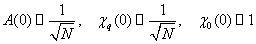
The condition for runaway can be found by studying the short-time evolution of the coherence equations leading to runaway solutions starting from the zero-field ground state. To this purpose we set the initial conditions as:
From the CE we easily obtain by differentiation:
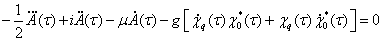
and introducing the initial conditions and making use of Equation (5) we find the equation which in the early stage of the process is linear:
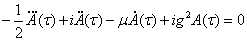
By searching for solutions of the form exp(ipτ) we arrive at the third-order algebraic equation for the exponent coefficient:
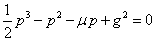
As clearly represented in Figure 1, there will be three real solutions or one real plus two complex conjugate solutions, depending on the values of g and µ. In the first case the dynamical evolution of the system remains stable and no runaway appears; in the second case a runaway will always be present, driving the system to a configuration totally different from the initial one. The minimal condition for runaway is found by requiring:
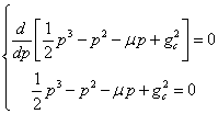
whose solution is
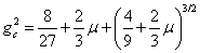
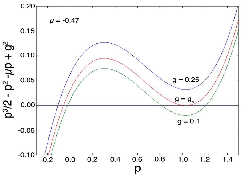
Figure 1.
Graphical representation of the behavior of Equation (15) for µ = −0.47 and for three different values of g. Note that when g = gc, the curve is tangential to the straight line y = 0. When g < gc, we get three real solutions and when g > gc, only one real solution exists, implying that there exist complex conjugate solutions, giving rise to runaway.
The condition for runaway is given by:  implying a threshold for density, since g2 depends on N/V. We are now in the position of finding the non-trivial solution (limit-cycle) towards which the system evolves and we will prove eventually that this energy is lower than zero.
implying a threshold for density, since g2 depends on N/V. We are now in the position of finding the non-trivial solution (limit-cycle) towards which the system evolves and we will prove eventually that this energy is lower than zero.3.2. Coherent Stationary Solutions
We now afford the solution of the coherence Equations (5,7) for liquid water. In this way we are able to derive the properties of the coherent state (liquid) as a function of the excited level involved in the molecule’s coherent oscillation. The selection of the specific excited level will be addressed in the next section. It should be stressed that once the conditions for runaway are met, an avalanche process drives the system from the zero-field configuration to a radically different quantum configuration, releasing an energy corresponding to the latent heat of vaporization to the environment [4]. Once this process is completed the dynamics of the system have dramatically changed. We are therefore interested to the determination of the coherent solutions after condensation has reached its stationary final configuration. The values of µ and g become renormalized by the process of condensation and by frequency renormalization. The stationary solution of the CE is found by writing the fields in a phase representation:
In Appendix A we derive explicitly such solutions by introducing the Ansatz Equation (18) into Equations (5,7–9). This solution will be expressed through an elegant geometrical method [15] by transforming the above equations into parametric equations. The solution is given by the intersection of the following parametric curves in the two-dimensional strip:
The complete solution for the amplitude of the fields and the energy gap Ecoh is given by the formula (see appendix A)
It is very easy to check, by combining the first four equations in and using some algebra, that

This equation tells us that the EM field oscillates in tune with the matter field. But our task is not complete yet. The photon mass term after condensation becomes substantially renormalized due to two important facts: frequency renormalization and migration of the initial quantum state from |0> to cosα |0> + sinα |q>. As said above, a new expression for µ must be considered, which depends on the parameters of the coherent solution. The new expression depends both on Ecoh and ωr, so that we end up with a highly non-linear system of equations that must be solved consistently. The renormalized expression, whose explicit calculation is described in Appendix B, contains not only the amplitudes f0n and f0(ω) connecting the molecule ground-state |0> to the excited states of the discrete and continuum spectrum respectively, but also the amplitudes fqn and fq(ω) connecting the excited partner in the coherent oscillation with the discrete and continuum spectrum. This necessity could give rise to possible troubles since these quantities are not known experimentally. Luckily, we will learn from the following analysis that the contribution of these unknown variables to the renormalized expression of µ in the case of water is negligible.
4. The Case of Liquid Water
We now apply the above general mathematical results to the particular case of liquid water.
4.1. Calculation of Critical Density for Water
The critical density dc of water is the minimal density at which water can exist as a liquid at thermodynamic equilibrium. It is reasonable to assume that such a condition corresponds in our theoretical framework to the minimal density at which a coherent state can exist at equilibrium. Since the coupling constant g depends on density, dc is the solution of the equation:
gc = g(dc) (21)
The condensation of the liquid occurs starting from the vapor. The first step, as discussed in the previous section, is the selection of the lasing mode, namely the mode coupled to the ground state by the coherent oscillation; we are still unable to identify it by a formal derivation, so that we will provisionally select the mode corresponding to the coherent solution which best describes the phenomenology.
First of all, we will evaluate the critical density for each excited level by using Equation (21). We will do that by introducing into Equation (21) the available experimental data on the oscillator strengths of water. The evaluation of µ in Equation (17) requires an experimental input (the UV spectrum of water) provided by Reference [16], to be inserted in Equations (10,11). We should note that the uppermost region of the discrete spectrum, ranging from 11.122 eV up to 12.62 eV (see Figure 7 of Reference [16]) has not been assigned in [16]. This is the consequence of the presence in this energy interval of a very large number of discrete levels gathering near the ionization threshold at 12.62 eV, each of them with a very low f-value. Being unable to distinguish among these closely packed lines, we have decided to treat such levels as if they were part of the continuum spectrum and we have called this contribution the continuum tail. Moreover, a few levels are simultaneously present in the same energy interval whose oscillator strength is substantially larger than average value and must therefore be taken into account as potential levels for coherence and assigned as discrete energy levels. We have been able to derive the oscillator strengths of the discrete peaks included in this region by an elaboration of the graph exhibited in Figure 7 of Reference [16]. To separate the contributions of the discrete and tail part of the spectrum in the region between 11.122 eV and 12.62 eV, we have made a few reasonable assumptions, accepting an error of the estimates in the range of 20%. We have estimated the continuum tail contribution in the region from 11.122 eV to 12.62 eV by assuming that the continuum tail starts just at the end of the first discrete peak at 11.3 eV (see Figure 2). Furthermore, by assuming a linear approximation and by requiring the continuity of f0(ω) and its derivative df0(ω)/dω at 12.62 eV, the continuum tail may be expressed by: f0(ω) = 0 (ω < 11.3 eV); f0(ω) = 0.0724ω − 0.81639 (ω < 11.85 eV) and f0(ω) = 0.108625ω − 1.2459 (ω < 12.62 eV).
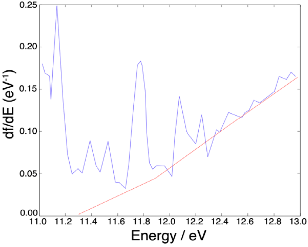
Figure 2.
Oscillator strength in the overlap (11–13 eV) between discrete and continuous UV-spectrum of the water molecule as reported in Figure 7 of Reference [16]. The red line indicates the extrapolation of the tail of the continuum spectrum.
This estimated tail should therefore be added to the experimental continuum spectrum above 12.62 eV quoted in Reference [16]. It turns out that the lower limit of the integral (Equation (11)) lies within the region of the discrete spectrum, giving rise for some levels to the appearance of a singularity of the type 1/(ω − ωq) . For these levels the integral should be understood as the well-known principal value integral. The discrete spectrum in the region from 11.122 eV to 12.62 eV is obtained by evaluating the peak heights p0n from the experimental curve after subtraction of the estimated continuum tail (Figure 3).
The last step is the calculation of the discrete f-values using the following argument. By using the Thomas-Reiche-Kuhn sum rule [14] and the value 0.3362 quoted in [16] as the sum of all the oscillator strengths of the levels below 12.62 eV we can write:

where f0(ω) is the above estimated tail. The oscillator strengths of the individual levels are derived by assuming that all the peaks in the unassigned region have a gaussian shape and an equal width so that in the region under investigation f0n = α∙p0n. It is easy to get α as:

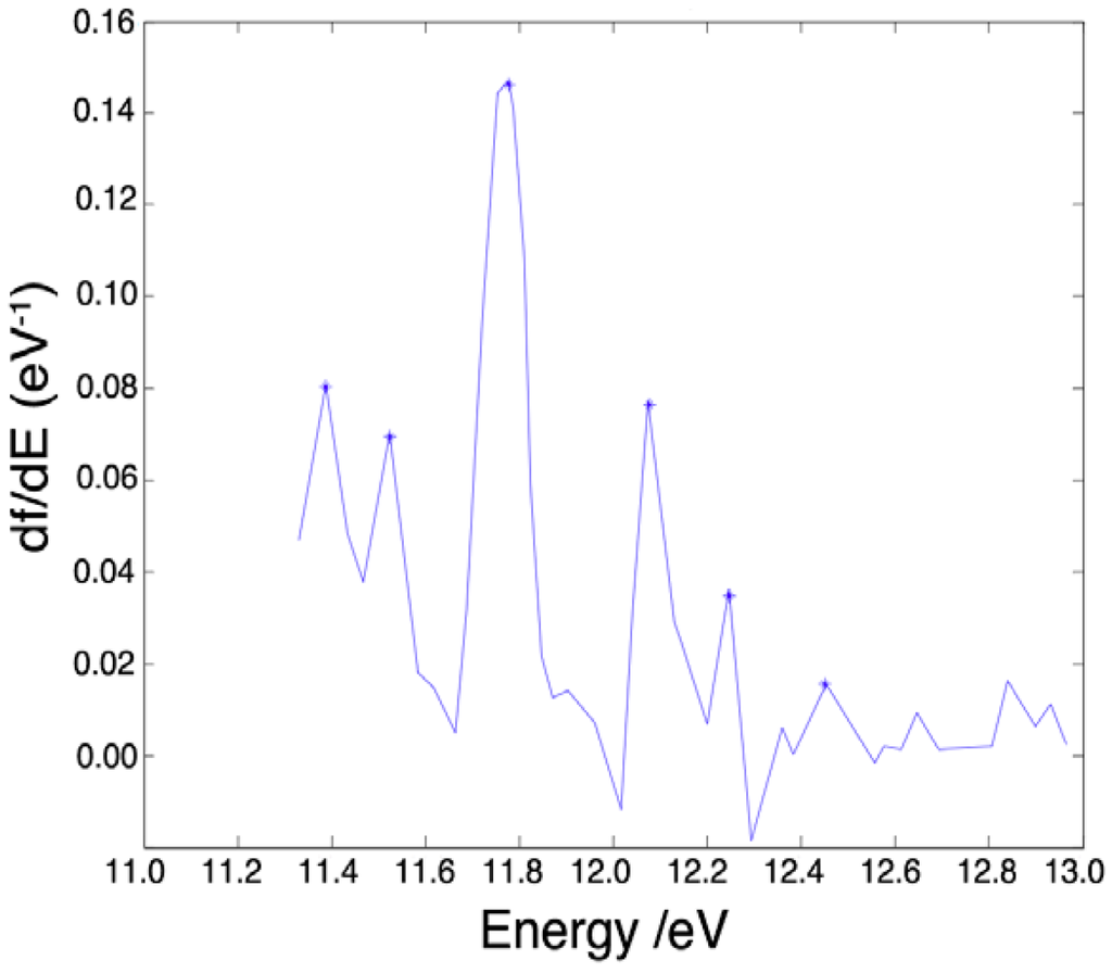
Figure 3.
Oscillator strength with continuum tail subtracted for the UV spectrum of the water molecule between 11 eV and 13 eV.
Since the above estimate could appear somehow arbitrary, we have checked a posteriori for the stability of the results by varying the straight line describing the tail. We have found that the differences always lie within the quoted uncertainty. The estimated values are shown in Table 1, where we also list the oscillator strengths of the levels below 11.12 eV given in Reference [16]. Coming back to the solution of Equation (21), the last problem is the evaluation of the contribution coming from the continuum spectrum. The integral Equation (11) between 12.62 eV and 200 eV is easily calculated by using the experimental data of Reference [16]. The contribution of the far spectrum above Ω = 200 eV has been shown to be negligible (of order 10−4) in Appendix C. In Table 2 we show the contribution to the mass photon term µ coming from the discrete spectrum, the continuum spectrum and the continuum tail, computed at the nominal density of 1 g∙cm−3.
The exact solution of Equation (21) for the various energy levels is given in Table 2, together with the estimate of the experimental uncertainty of the critical densities. Please note that all the physical quantities shown in Table 2 are calculated at the critical density. From Table 2 we see that all the levels have critical densities in the range of the experimental value 0.322 g∙cm3 of liquid water. The level at 12.07 eV, which we are going to show as the likeliest on phenomenological grounds, has a critical density quite close to the experimental value. Actually a coherent state produced by the oscillation between the ground state and this level would include a plasma of very loosely bound electrons whose energy per particle reaches a value slightly lower than the ionization threshold (12.62 eV). This property would account for the appearance of the relevant phenomenon of electron transfer occurring in water and aqueous systems, which is particularly important in living organisms [17]. For these reasons we should presume that the level at 12.07 eV is the winner of the competition among levels for the self-production of the cavity where the coherent field becomes self-trapped. In a future publication we will address the derivation from first principles of the selection of such a level.

Table 1.
Contribution to the mass photon term µ coming from the discrete spectrum, the continuum spectrum and the continuum tail, computed at the nominal density of 1 g∙cm−3. The oscillator strengths and the coupling constants g2 are also given for completeness.
| ωq | f | g2 | µ0 | µc | µtail | µ |
|---|---|---|---|---|---|---|
| 7.400 | 0.0500 | 0.264 | −0.279 | −0.853 | −0.053 | −1.185 |
| 9.700 | 0.0732 | 0.225 | −0.384 | −1.028 | −0.092 | −1.504 |
| 10.000 | 0.0052 | 0.015 | 0.225 | −1.064 | −0.104 | −0.943 |
| 10.170 | 0.0140 | 0.039 | 0.130 | −1.087 | −0.113 | −1.070 |
| 10.350 | 0.0107 | 0.029 | 0.243 | −1.114 | −0.123 | −0.994 |
| 10.560 | 0.0092 | 0.024 | 0.133 | −1.149 | −0.139 | −1.155 |
| 10.770 | 0.0069 | 0.017 | −0.068 | −1.188 | −0.161 | −1.418 |
| 11.000 | 0.0218 | 0.052 | −0.297 | −1.238 | −0.198 | −1.733 |
| 11.120 | 0.0223 | 0.052 | 0.698 | −1.267 | −0.227 | −0.796 |
| 11.385 | 0.0098 | 0.022 | 0.381 | −1.343 | −0.359 | −1.321 |
| 11.523 | 0.0086 | 0.019 | 0.521 | −1.389 | −0.381 | −1.250 |
| 11.772 | 0.0178 | 0.037 | 0.486 | −1.492 | −0.362 | −1.368 |
| 12.074 | 0.0101 | 0.020 | 0.501 | −1.558 | −0.384 | −1.441 |
| 12.243 | 0.0053 | 0.010 | 0.626 | −1.437 | −0.569 | −1.381 |
| 12.453 | 0.0025 | 0.005 | 0.551 | −1.089 | −0.923 | −1.461 |
Table 2.
Critical molar volumes and densities for the various discrete transitions of water. Values in brackets represent estimated standard errors.
| Energy (eV) | g2 | gc2 | µ | Vmolcrit (cm3) | dcrit (g∙cm3) |
|---|---|---|---|---|---|
| 7.40 | 0.092 | 0.092 | −0.41(1) | 52(1) | 0.35(1) |
| 9.70 | 0.065 | 0.065 | −0.44(1) | 62(2) | 0.29(1) |
| 10.00 | 0.008 | 0.008 | −0.49(10) | 34(7) | 0.52(10) |
| 10.17 | 0.018 | 0.017 | −0.48(5) | 40(5) | 0.45(5) |
| 10.35 | 0.014 | 0.014 | −0.49(5) | 37(4) | 0.49(5) |
| 10.56 | 0.010 | 0.010 | −0.49(4) | 42(3) | 0.42(3) |
| 10.77 | 0.006 | 0.006 | −0.49(3) | 52(3) | 0.35(2) |
| 11.00 | 0.015 | 0.014 | −0.49(4) | 64(5) | 0.28(2) |
| 11.12 | 0.031 | 0.031 | −0.47(7) | 31(5) | 0.59(9) |
| 11.38 | 0.008 | 0.008 | −0.49(3) | 48(3) | 0.37(2) |
| 11.52 | 0.007 | 0.007 | −0.49(3) | 46(3) | 0.39(3) |
| 11.77 | 0.013 | 0.013 | −0.49(2) | 51(2) | 0.36(1) |
| 12.07 | 0.007 | 0.007 | −0.49(2) | 53(2) | 0.34(1) |
| 12.24 | 0.004 | 0.004 | −0.50(2) | 50(2) | 0.36(1) |
| 12.45 | 0.002 | 0.001 | −0.50(1) | 53(1) | 0.34(1) |
4.2. Coherent Ground-State of Liquid Water
In this subsection, and in the particular case of water, we discuss the solutions Equation (20) of Equations (5,7) that define the coherent stationary-state that the water system approaches after runaway. As noted at the end of Section 3, we have to re-determine the parameter µ. First of all, we observe (see Appendix D) that the contribution of µr,cont is negligible after renormalization. The only possible contribution to the photon mass term comes from singularities appearing in the discrete sum of Equation (B5). In order to evaluate this sum we show at first by a general argument that

must be substantially smaller than ωq. The numerical value of the 1-component of Γ in Equation (19) cannot be lower than Γmin = −1/4. Therefore we get from the graphical solution of Equation (19) (see Figure 5) that:

The third-order inequality has the approximated solution:

where use has been made of the smallness of g2. The parameter

cannot exceed the limiting value g2ωq and therefore is so small with respect to all the excitations ωn to make all the denominators appearing in the sum Equation (B5) large enough to allow us to neglect the corresponding terms, except for the term proportional to f0q, whose denominator could be made to vanish by the physical condition:

In conclusion we get:

We are equipped now with the theoretical tools necessary for the calculation of the self-consistent condition. Starting from the lowest possible value of the photon mass µ = −0.5, we look for which couple of values  Equation (19) are simultaneously satisfied (Γ1 − Ψ1 = 0 = Γ2 − Ψ2). This may be done in MATLAB with the built-in numerical solver FSOLVE or by using multidimensional secant methods such as Broyden’s algorithm. The values of x and
  obtained may now be reported in Equation (20) in order to retrieve the values of sin2α, Ecoh and ωr. Inserting these three new values into Equation (27) allows the computation of µr(ωr). If this value is negative, a small positive increment ε is added to the starting µ-value and a new cycle (µ + ε) → → (sin2α, Ecoh, ωr) → µr(ωr) is performed until a positive value of µr(ωr) is obtained. As shown in Figure 4, this positive value means that Equation (26) has been satisfied with an accuracy given by the chosen increment ε.
Equation (19) are simultaneously satisfied (Γ1 − Ψ1 = 0 = Γ2 − Ψ2). This may be done in MATLAB with the built-in numerical solver FSOLVE or by using multidimensional secant methods such as Broyden’s algorithm. The values of x and obtained may now be reported in Equation (20) in order to retrieve the values of sin2α, Ecoh and ωr. Inserting these three new values into Equation (27) allows the computation of µr(ωr). If this value is negative, a small positive increment ε is added to the starting µ-value and a new cycle (µ + ε) → → (sin2α, Ecoh, ωr) → µr(ωr) is performed until a positive value of µr(ωr) is obtained. As shown in Figure 4, this positive value means that Equation (26) has been satisfied with an accuracy given by the chosen increment ε. Figure 5 shows the graphical solution corresponding to the choice of the level at 12.07 eV as the excited partner of the ground state in the coherent oscillation, while the calculated values are shown in Table 3. The values corresponding to this particular level are different from the ones given in Reference [4] due to the different values of oscillator strengths we have used. Nevertheless, the differences do not change the global landscape of the predicted features. It is worth noting that a negative value is obtained for Ecoh, completing the demonstration that the non-coherent gas-like state becomes unstable above a critical density. In Table 3 we have also listed the values of the critical densities and of the energies of the coherent states that would emerge from a hypothetical coherent oscillation between the ground state of the water molecule and each excited level of the UV spectrum. We can see that the energy of the state corresponding to the level at 12.07 eV, which is at present our preferred candidate for playing the role, is reasonable according to the thermodynamic evaluations given in Reference [4].
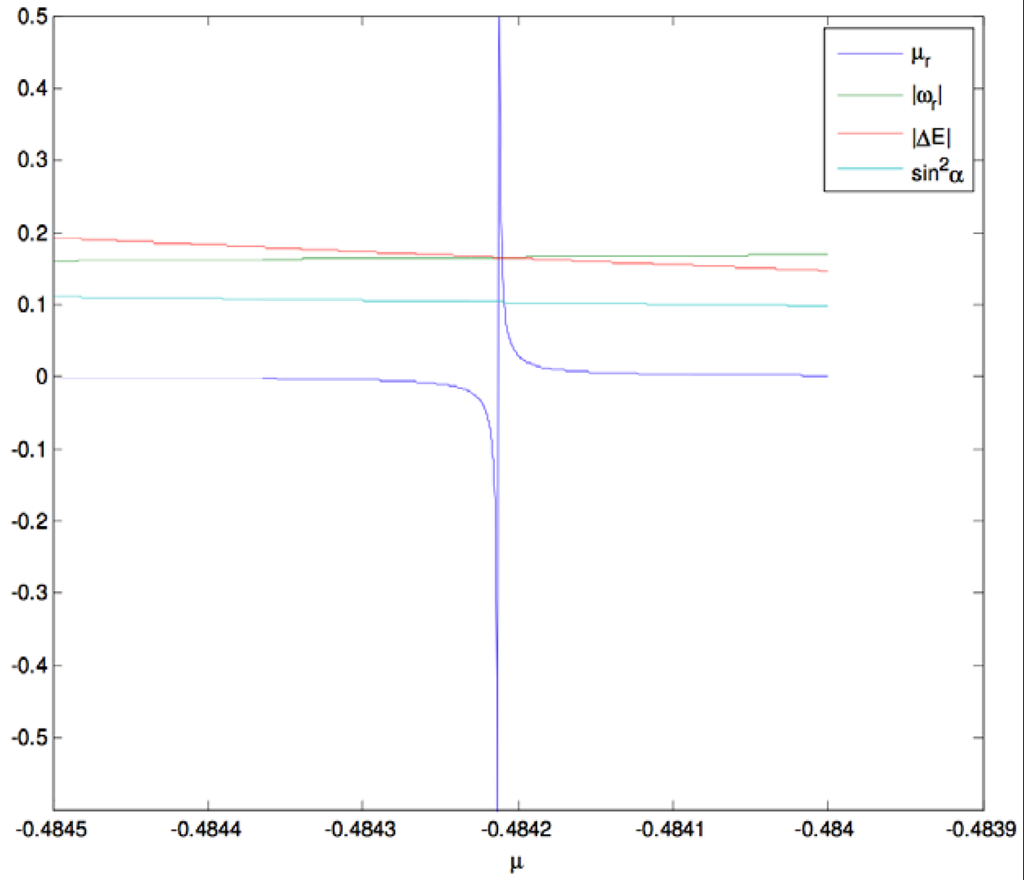
Figure 4.
Variation of the computed solution as a function of the running µ.
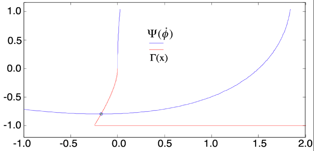
Figure 5.
Self-consistent space-independent solution of Equation (19)  for the level E = 12.07 eV with a coherent coupling constant g2 = 0.02, an electron plasma frequency ωp= 6.7783 eV and a renormalized photon mass µr = −0.48425.
for the level E = 12.07 eV with a coherent coupling constant g2 = 0.02, an electron plasma frequency ωp= 6.7783 eV and a renormalized photon mass µr = −0.48425.
Table 3.
Solutions of the coherence equations for each discrete excited level ωq of the water molecules and associated coherent energies Ecoh and critical densities dcrit.
| ωq | g2 | μr | x | φ | A0 | sin2α | ωr | Ecoh (eV) | dcrit (g.cm-3) |
|---|---|---|---|---|---|---|---|---|---|
| 7.400 | 0.264 | −0.3589 | 1.457 | 1.091 | 1.55 | 0.22 | 0.672 | −0.67(17) | 0.348(8) |
| 9.700 | 0.225 | −0.3759 | 1.403 | 1.082 | 1.60 | 0.21 | 0.795 | −0.79(10) | 0.290(7) |
| 10.000 | 0.015 | −0.4879 | 0.713 | 1.011 | 2.94 | 0.09 | 0.107 | −0.11(4) | 0.522(102) |
| 10.170 | 0.039 | −0.4715 | −0.909 | 1.023 | −2.36 | 0.13 | 0.238 | −0.24(3) | 0.451(51) |
| 10.350 | 0.029 | −0.4781 | −0.843 | 1.019 | −2.52 | 0.12 | 0.192 | −0.19(6) | 0.489(51) |
| 10.560 | 0.024 | −0.4815 | −0.804 | 1.016 | −2.64 | 0.11 | 0.168 | −0.17(5) | 0.424(32) |
| 10.770 | 0.017 | −0.4864 | 0.736 | 1.012 | 2.86 | 0.10 | 0.129 | −0.13(4) | 0.348(23) |
| 11.000 | 0.052 | −0.4634 | −0.978 | 1.029 | −2.21 | 0.14 | 0.322 | −0.32(10) | 0.280(21) |
| 11.120 | 0.052 | −0.4634 | −0.978 | 1.029 | −2.21 | 0.14 | 0.325 | −0.33(10) | 0.590(92) |
| 11.385 | 0.022 | −0.4828 | −0.787 | 1.015 | −2.69 | 0.11 | 0.168 | −0.17(6) | 0.372(24) |
| 11.523 | 0.019 | −0.4850 | −0.757 | 1.013 | −2.78 | 0.10 | 0.151 | −0.15(5) | 0.394(25) |
| 11.772 | 0.037 | −0.4728 | 0.897 | 1.023 | 2.38 | 0.13 | 0.265 | −0.27(8) | 0.356(13) |
| 12.074 | 0.020 | −0.4842 | −0.767 | 1.014 | −2.75 | 0.10 | 0.165 | −0.16(5) | 0.342(12) |
| 12.243 | 0.010 | −0.4916 | 0.642 | 1.008 | 3.23 | 0.08 | 0.093 | −0.09(2) | 0.359(13) |
| 12.453 | 0.005 | −0.4956 | −0.535 | 1.004 | −3.80 | 0.06 | 0.051 | −0.05(1) | 0.341(8) |
5. Discussion and Outlook
Let us now compare the results of our theoretical approach with the phenomenology of water. In this paper we have not addressed the problem of temperature, which is extensively discussed in [4]; the present discussion holds rigorously at T = 0. In previous articles [4,18,19,20,21] we have calculated the thermodynamic quantities for a liquid corresponding to the choice of the level at 12.07 eV and we have found a good agreement with the observations, including density and specific heat. However the main element to be taken into account is the property of water in biological organisms to release electrons. This property cannot be understood in the conceptual framework where water molecules are assumed to be uncorrelated and subjected only to mutual static interactions. In this case the excitation of each molecule cannot be larger than a couple of eVs, much smaller than the ionization threshold which is at 12.62 eV. On the contrary, in our approach, when we choose as excited partner in the coherent oscillation the level at 12.07 eV, each coherent molecule would produce during its oscillation a quasi-free electron, very weakly bound. The ensemble of these electrons would be very easily excitable, giving rise to collective coherent excitations (vortices) which are able to explain a large number of biological phenomena arising as a consequence of the possibility of having an electron transfer in aqueous systems. This circumstance strongly suggests that the level to be chosen for the coherent oscillation is the one at 12.07 eV. Other candidate levels would give rise to a liquid having a higher density due to the smaller molecular volume in the excited state and to a much smaller ability to release electrons. The determination of the thermodynamic and electromagnetic variables (specific heat, viscosity, dielectric permittivity and so on) of liquid water would allow us to test the predictive power of this approach. As a first example, properties of water glasses at low temperature have been analyzed [19] and found in good agreement with the observed facts. Finally, we want to stress that since the parameters g and µ controlling the onset of coherence for different choices of the excited level depend on the thermodynamic parameters, our approach allows the appearance of different phases of liquid water corresponding to the choice of different excited levels. This opens the way to discuss the thorny problem of the existence of more than one phase of liquid water at low temperature.
Appendix A
In this Appendix we evaluate the non-trivial limit cycle of CE (minimum energy state) by using a method introduced in [4]. We re-write here Equations (5,7)

Together with the constants of motion, which are in our case the ‘total momentum’ Q and the Hamiltonian H (see [4], [11]):


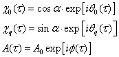
We now introduce the Ansatz, which accounts for the fact that the fields are complex functions:

into the first two Equation (A1) and we get:

By equating separately the modulus and the phase factors in Equation (A5), we realize that  and
and  do not depend on τ so that
  . Moreover, the exponential factor on the RHS of Equation (A5) should be real and equal to ±1 only. We have therefore:
and do not depend on τ so that . Moreover, the exponential factor on the RHS of Equation (A5) should be real and equal to ±1 only. We have therefore:
These two conditions imply that:
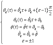
where ϑ0 and ϑq are arbitrary integration constants. Equation (A5) may then be rewritten in the following form:

By making use of the Ansatz Equation (A4) for the EM field we get:

We replace Equation (A9) into the third Equation (A1) and get:


We replace now the Ansatz Equation (A4) into the Equation (A2) getting:

Equations (A11,A12) can be rewritten in the following form:

Now, as  ,
,  , so that
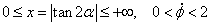
  , and with 0 ≤ x ≤ +∞, the solution of this system is therefore given by the intersection of two parametric curves defined by:
, , so that , and with 0 ≤ x ≤ +∞, the solution of this system is therefore given by the intersection of two parametric curves defined by: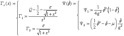
The constants of motion Equations (A2,A3) are fixed by the boundary conditions and are constant in time provided that the ground state is stable. During the transition from the non-coherent to the coherent state dissipative processes occur which temporarily spoil the Hamiltonian dynamics, implying that the transition should occur through the release of heat. Therefore, we expect that Q should not change during the transition and H should vary by a negative amount. We set Q = 0, considering that the conditions before runaway are A = χq ≡ 0, meaning that the field is zero and no molecules are excited. By replacing Equation (A4) into Equation (A2), we get:

Similarly one gets from Equation (A3):

By making use of the third Equation (A1) we obtain:

Inserting Equation (A17) into Equation (A16) we finally get:

that gives the energy of the coherent state in the scale where the energy of the non-coherent state is zero. Please note that Equation (A18) is the sum of three terms, two of which are positive and one negative. It turns out by numerical calculation that the negative term corresponding to the matter-field interaction term is large enough to compensate for the contribution of the positive terms that corresponds to the energy of the EM field and matter excitation energy, so that the total energy is negative.
Appendix B
In this appendix we derive the renormalized expression µr for the parameter µ in the lowest-energy coherent state. The calculation is performed by using the Natural Unit System (NU) where h = 2π and c = 1, so that the energy E becomes equal to the pulsation ω = 2πν. As explained in [11], the photon mass term is defined by:

where the state |coh> is the coherent state and can be written in terms of single-particle states as:

Please note that, as has been done in the pre-runaway case, the sum in Equation (B1) must be extended to both the discrete and continuum spectrum in order to fulfill completeness of intermediate states. Actually the sum in Equation (B1) will contain a sum of discrete terms and an integral over unbounded intermediate states. By substitution of Equation (B2) into Equation (B1) we find:

By making use of the definition of oscillator strength [14]:

we can express Equation (B3) as:

The explicit form of µr,cont is given by:

Appendix C
The contribution coming from the far spectrum is given by (Ω = 200 eV):

By making the asymptotic ansatz:

Stemming from high-energy scaling of cross-sections in QED, we have:

We compute the integral

where we have neglected the small contribution of ε = Ecoh/Ω and η = ωr/Ω. We obtain finally:

totally negligible in our approximation.
Appendix D
In this appendix we evaluate the contribution of the continuum spectrum of water to the renormalized value of the parameter µ in the coherent state. This contribution turns out to be negligible. We have:

where the Thomas-Reiche-Kuhn sum rule has been used. The coefficient in Equation (B6) is given by:

An upper bound for the absolute value of Equation (B6) is finally given by:

a negligible quantity. This solves the problem arising from the lack of experimental knowledge of fq(ω).
References
- Franks, F. Water: A Comprehensive Treatise; Plenum Press: New York, NY, USA, 1982. [Google Scholar]
- Teixeira, J.; Luzar, A. Physics of liquid water: Structure and dynamics. In Hydration Processes in Biology: Theoretical and Experimental Approaches (NATO ASI series A); Bellissent-Funel, M.C., Ed.; IOS Press: Amsterdam, the Netherlands, 1999; pp. 35–65. [Google Scholar]
- Bertolini, D.; Cassettari, M.; Ferrario, M.; Grigolini, P.; Salvetti, G.; Tani, A. Diffusion effects of hydrogen bond fluctuations. I. The long time regime of the translational and rotational diffusion of water. J. Chem. Phys. 1989, 91, 1179–1190. [Google Scholar] [CrossRef]
- Arani, R.; Bono, I.; del Giudice, E.; Preparata, G. QED coherence and the thermodynamics of water. Int. J. Mod. Phys. B 1995, 9, 1813–1841. [Google Scholar] [CrossRef]
- Collini, E.; Wong, C.Y.; Wilk, K.E.; Curmi, P.M.G.; Brumer, P.; Scholes, G.D. Coherently wired light-harvesting in photosynthetic marine algae at ambient temperature. Nature 2010, 463, 644–647. [Google Scholar]
- Scholes, G.D.; Curutchet, C.; Mennucci, B.; Cammi, R.; Tomasi, J. How solvent controls electronic energy transfer and light harvesting. J. Phys. Chem. B 2007, 111, 6978–6982. [Google Scholar]
- Bockris, J.M.; Khan, S.U.M. Bioelectrochemistry; Plenum Press : New York, NY, USA, 1993; pp. 696–697. [Google Scholar]
- Jaynes, E.T. Maximum Entropy and Bayesian Methods; Skilling, J., Ed.; Klüwer Academic Publishers: Dordrecht, the Netherland, 1989; pp. 1–27. [Google Scholar]
- Del Giudice, E.; Spinetti, P.R.; Tedeschi, A. Water dynamics at the root of metamorphosis in living organisms. Water 2010, 2, 566–586. [Google Scholar] [CrossRef]
- Lamb, W.E.; Retherford, R.C. Fine structure of the hydrogen atom by a microwave method. Phys. Rev. 1947, 72, 241–243. [Google Scholar] [CrossRef]
- Preparata, G. QED Coherence in Matter; World Scientific: Toh Tuck, Singapore, 1995. [Google Scholar]
- Kurcz, A.; Capolupo, A.; Beige, A.; del Giudice, E.; Vitiello, G. Energy concentration in composite quantum systems. Phys. Rev. A 2010, 81, 063821:1–063821:5. [Google Scholar]
- Kurcz, A.; Capolupo, A.; Beige, A.; del Giudice, E.; Vitiello, G. Rotating wave approximation and entropy. Phys. Lett. A 2010, 374, 3726–3732. [Google Scholar] [CrossRef]
- Hilborn, R.C. Einstein coefficients, cross sections, f values, dipole moments, and all that. Am. J. Phys. 1982, 50, 982–986. [Google Scholar]
- Gamberale, L. Quantum Theory of the Electromagnetic Field in Interaction with Matter. Unpublished work, 2001. [Google Scholar]
- Chan, W.F.; Cooper, G.; Brion, C.E. The electronic spectrum of water in the discrete and continuum regions. Absolute optical oscillator strengths for photoabsorption (6–200 eV). Chem. Phys. 1993, 178, 387–400. [Google Scholar] [CrossRef]
- Marcus, R.A. Electron transfer reactions in chemistry: theory and experiment (Nobel lecture). Angew. Chem. 1993, 32, 1111–1222. [Google Scholar] [CrossRef]
- Del Giudice, E.; Galimberti, A.; Gamberale, L.; Preparata, G. Electrodynamical coherence in water: A possible origin of the tetrahedral coordination. Mod. Phys. Lett. B 1995, 9, 953–958. [Google Scholar] [CrossRef]
- Buzzacchi, M.; del Giudice, E.; Preparata, G. Coherence of the glassy state. Int. J. Mod. Phys. B 2002, 16, 3761–3786. [Google Scholar]
- Del Giudice, E.; Tedeschi, A. Water and the autocatalysis in living matter. Electromagn. Biol. Med. 2009, 28, 46–54. [Google Scholar] [CrossRef]
- Marchettini, N.; del Giudice, E.; Voeikov, V.L.; Tiezzi, E. Water: A medium where dissipative structures are produced by a coherent dynamics. J. Theor. Biol. 2010, 265, 511–516. [Google Scholar] [CrossRef]
© 2012 by the authors; licensee MDPI, Basel, Switzerland. This article is an open-access article distributed under the terms and conditions of the Creative Commons Attribution license (http://creativecommons.org/licenses/by/3.0/).