
Multi-Objective Design of a Horizontal Flow Subsurface Wetland

1
Environmental Laboratory, Autonomous University of Tlaxcala, Clzda Apizaquito S/N, km. 1.5, Apizaco 90300, Tlaxcala, Mexico
2
Department of Electronics, Autonomous University of Tlaxcala, Clzda Apizaquito S/N, km. 1.5, Apizaco 90300, Tlaxcala, Mexico
*
Author to whom correspondence should be addressed.
†
These authors contributed equally to this work.
Water 2024, 16(9), 1253; https://doi.org/10.3390/w16091253
Submission received: 28 March 2024
/
Revised: 19 April 2024
/
Accepted: 24 April 2024
/
Published: 27 April 2024
(This article belongs to the Section Water Quality and Contamination)
Abstract
:An artificial wetland is used to treat gray, waste, storm or industrial water. This is an engineering system that uses natural functions of vegetation, soil and organisms to provide secondary treatment to gray water. In the physical design of each artificial wetland, there are various action factors that must meet certain characteristics so that the level of gray-water pollution is reduced. In this sense, several design methodologies have been developed and reported in the literature, but some are customized designs and often do not meet the required decontamination objectives. This challenge increases as the complexity of the task in its structure also increases. Particularly in this work, a multi-objective evolutionary algorithm is used to optimize the physical design of a horizontal flow subsurface wetland (HFSW) for gray-water treatment. The study aims to achieve two objectives: first, to minimize the physical volume, and second, to maximize the contaminant removal efficiency. The defined objective functions depend on six design variables called hydraulic retention time, width, length, water depth inside the wetland, substrate depth and slope. Three constraint functions are also defined: removal efficiency greater than 95%, physical volume below 500 m3 and compliance with a length–width ratio is 3:1, varying the population size and number of generations equal to 200, 400, and 600. The set of solutions according to the number of generations as well as the Pareto front corresponds to the best solution that complies with the constraints of the problem of oversizing the HFSW, and the Pareto front shows the interaction between the objectives and their behavior, reflecting the problem’s nature as minimization–maximization.
1. Introduction
Pollution aggravates various environmental problems such as water scarcity, soil erosion and atmospheric drought. The treatment of water resources is increasingly important, and wastewater treatment processes are sought to be efficient and effective [1]. On the one hand, green technologies are still developing to provide sustainable solutions to the problems of pollution. On the other hand, constructed wetlands technology is an established green multi-purpose option for water management and wastewater treatment, with numerous effectively proven applications worldwide and with multiple environmental and economic advantages. These systems can operate as water treatment plants, habitat creation sites, urban wildlife refuges, recreational or educational facilities, landscape engineering and ecological art areas [1,2,3]. Note that conventional wastewater treatment systems are less efficient in removing recalcitrant compounds and color. In response to this problem, constructed wetlands could be one option for domestic and industrial wastewater treatment [4,5] since these systems are simple and have proved to be sustainable and green technology to improve wastewater quality [2]. However, despite its simplicity, this is a multi-objective optimization problem [3,6,7]. In this way, Ikenberry et al. [8] addressed the problem of groundwater wastewater in Murdoc, Nebraska, by implementing a surface flow constructed wetland (SFW). The main target of this paper was to optimize the carbon tetrachloride remediation process, while safeguarding adjacent properties from potential flooding and channel instability. However, in order to increase the biodiversity of the SFW, deeper excavations were carried out, resulting in the configuration of a bottom with undulating characteristics. This last particularity caused an increase in the hydraulic retention time and, therefore, in the sizing of the SFW. Huang et al. [9] used the SubWet 2.0 numerical model to model and analyze the treatment efficiency of vertical flow constructed wetlands. The SubWet 2.0 model uses, as design input values, the width, length, depth, precipitation factor, slope, average percentage of wetland particles, hydraulic conductivity and flow, in addition to specifying the type of natural or artificial wetland. Once the parameters are established, the model computes the area, volume, hydraulic head, recommended horizontal flow, recommended flow, flow width and number of channels. Further, it is capable of simulating the elimination of biochemical oxygen demand (BOD5), ammonium nitrogen, nitrate nitrogen and total phosphorus (TP). To evaluate the modeling performance, in terms of these pollutants, use the correlation coefficient and the Nash–Sutcliffe efficiency coefficient. However, it only provides one design for each simulated wetland without applying optimization techniques for area reduction. Furthermore, the simulation start parameters are fixed, which does not allow exploring other designs. As a consequence, the simulation time is conditioned by the input data, which can cause very fast or very slow simulations. Andreo et al. [10], examines the removal efficiency of five pollutants: BOD5, TP, chemical oxygen demand, total suspended solids and total nitrogen in a horizontal flow subsurface wetland (HFSW). Since the HFSW experiences bed drying problems due to oversizing and high evapotranspiration in the area, a theoretical resizing of the HFSW is proposed using the Reed model. However, although the input data for optimization are obtained in the field, which increases the reliability, the Reed model only provides a single design, which must be adjusted only to the initial operating conditions of the HFSW, limiting thus the exploration of new design proposals. Liao et al. [11] reported the study of one of the main drainage channels of Beijing, which is the Beiyun River in China, where 76% of the city’s total wastewater is discharged into this river. To improve the ecological environment and water quality of the river, an artificial wetland was designed and built in the lower part of the river. In the evaluation and optimization process, the MIKE 21 modeling system was used to simulate the water distribution system. Furthermore, a back-propagation neural network was trained to quantify the relationship between hydrological parameters and the overall performance of the constructed wetland based on its water distribution characteristics and their corresponding scores. A genetic algorithm was used for optimizing the water control, which determines an optimal strategy that combines the flow and water level parameters of the artificial wetland. Water quality was simulated by applying chemical oxygen demand as a pollutant index to reflect the water quality of the surface flow zone with an estimated initial concentration of 25.6 mg/L. Despite the complexity of the simulation and optimization process, which involved the use of three different software’s, the study lacked the graphical presentation of the generations carried out to visualize all the solutions. Likewise, an approximate simulation time of 24 h was reported, which highlights the need to consider temporal aspects in this type of analysis.
As can be seen in the papers reported to date [4,5,8,9,10,11,12], all artificial wetlands, designed and some already built, use different design methodologies, but none of them address the problem from a multi-objective optimization approach. This is a serious drawback since the structure of said artificial wetland differs substantially from reality. For these reasons, some artificial wetlands not only consume many financial resources during their construction and maintenance but also do not ensure that wastewater treatment is the most effective. In fact, several artificial wetlands are inoperative when their capacities are exceeded, and this is due to incorrect design planning. As a consequence, its repair is more expensive than the construction of a new artificial wetland but now considering the new challenges. Note that this process follows a trial-and-error design methodology, increasing construction costs, which is not viable from an economic point of view. With this in mind, this paper presents the use of the NSGA-II algorithm to optimize the design of an HFSW for gray-water treatment. In particular, two objectives are optimized: the minimization of the physical volume () and the maximization of the contaminant removal efficiency (). Hence, the design of the HFSW is formulated as a multi-objective optimization problem. The Pareto front generated by the two targets is very similar to that reported in the literature, showing the effectiveness of the optimizer. As an example, a Pareto front solution is selected, and as a consequence, the numerical value of the HFSW design variables is obtained. The NSGA-II algorithm can play a crucial role in the built wetland, providing tools for data-driven decision making and implementing sustainable management practices and strategy to the peculiarities of the HFSW. The manuscript is organized as follows: Section 2 describes the behavior equations of the HFSW. The objective functions, constraints and the search space are also defined. A flowchart of the operation of NSGA-II algorithm is briefly described in Section 3. Numerical results are discussed in Section 4, showing the generated Pareto front by the two objectives defined above. By selecting a point on the generated Pareto front, the design variables can be automatically obtained with the target of building the HFSW a posteriori. Section 5 presents a brief discussion about the multi-objective optimization of the HFSW. Finally, the conclusions are summarized in Section 6.
2. HFSW Behavior Model
A detailed description of the method used for optimizing a HFSW, from mathematical modeling, is here described. The design of the HFSW is optimized using the NSGA-II algorithm, based on the adequate selection of equations that describe the behavior of the HFSW to subsequently define the objectives, constraints and design variables. Thus, the goal is to minimize and maximize simultaneously.
2.1. Behavior Equations
The design of artificial HFSW involves two stages. The first stage entails kinetic design, and a first-order model is given by [12,13]
where is the first-order kinetic constant [d−1], [mg/L] and [mg/L] are the input–output concentrations of the pollutant, respectively, and t is the hydraulic retention time [d]. The second stage involves hydraulic design, which takes into account the superface area () [m2] given by
where Q is the flow rate [m3/d], is the substrate depth [m] and n is the porosity. The width (W) [m] can be approximated as
where is the water depth [m], s is the slope [%] and is the hydraulic conductivity [m/d]. The length (L) [m] is approximated as
2.2. Objective Functions
On the one hand, a drawback in the construction of artificial HFSW is that they require large areas [4,5], consuming many financial resources during their construction and maintenance, and they do not ensure that the wastewater treatment is effective. On the other hand, in the multi-objective optimization process, the objective functions to be optimized must meet two main characteristics: firstly, the objectives depend on the design variables and satisfy the design constraints; secondly, there is a trade-off between them [14]. With this in mind and from (1)–(4), the targets are defined as
Therefore, this study aims to minimize [m3] while maximizing [%] at the outlet of the HFSW and satisfying all required constraints.
2.3. Design Variables and Constraints
2.3.1. Design Variables
In a multi-objective optimization problem, the design variables, also called decision variables, have an impact on the solution of the optimization problem since during the optimization process, one must find the best combination of design variables that optimizes the designer’s preference and maintains certain requirements or constraints. In this sense, Table 1 shows the design variables to be used during the optimization process along with the range of values according to the literature [15,16,17]. Note that the behavior of the two objective functions given by (5) and (6) depends on the design variables. However, to improve the search for solutions, in this work, the search space is expanded, and this is achieved by expanding the range of each design variable. The range of each design variable is deduced by experimentation. It is worth mentioning that the value of n and are obtained from [13,16].
2.3.2. Constraints
An objective function cannot be optimized infinitely since its performance is often limited by the presence of constraints. Thus, a constraint function is also expressed mathematically in terms of design variables. Basically, a constraint function can be an inequality or equality constraint. For this work, three constraints are defined: the first must ensure the contaminant removal with 95% efficiency. The second refers to obtaining an optimized physical volume less than 500 m3. The third constraint must satisfy the relation of 3:1 between L and W [13,16]. Thus, the constraint functions are defined as
3. Multi-Objective HFSW Design Methodology
On the one hand, a multi-objective optimization problem can mathematically be formulated as
where f(x) is the vector with n objective functions, c(x) is the vector with k constraint functions, and x is the vector with q design variables on the decision space X, limiting each design variable between the lower () and upper () limits. On the other hand, the NSGA-II method is a powerful decision space exploration engine based on genetic algorithms for solving multi-objective optimization problems as described by (10) in general and the use of (5)–(9) and the design variables of Table 1 in particular. The NSGA-II operates under four main principles: non-dominated sorting, elite preserving operator, crowding distance and selection operator. Under these principles, the NSGA-II algorithm executes the search for the best solutions of the HFSW design according to the design variables, taking a population of parents. This population undergoes an operational cycle, where individuals are adjusted within the problem’s constraints. Once the solutions are found, they are appended according to the number of generations until forming an optimal set and satisfying the problem’s solutions. The results of the design variables found by NSGA-II are attached to the last computed generation, forming the non-dominated solutions. The behavior of this set of solutions is verified by confronting the objectives and comparing the maximization–minimization result to form the Pareto front [18]. Since NSGA-II is coded to minimize objective functions, any objective function can easily be converted to a maximization problem by multiplying the objective function by −1. Figure 1 shows a flowchart for the execution of the algorithm. On this diagram, whereas the design variables are used to generate the initial population and their descendants in the second and third step, respectively, in the fourth step, the objective and constraints functions defined by (5)–(9) are evaluated.
4. Numerical Results
Numerical results for optimizing an HFSW are presented. The tests were conducted by using a CPU with 1.6 GHz Intel core i5 and memory size 4 GB.
4.1. Found Solutions
The NSGA-II algorithm generates acceptable solutions based on population size (P), the number of generations (G), defined constraints and the search space defined by the design variables given in Table 1. Table 2 shows four solutions of the last generation for different values of P and G.
From the third column of Table 2, > 0.95 (or as a percentage > 95%), ensuring not only a value of 20 mg/L of BOD5 at the outlet of the HFSW but also complying with the NOM-003-SEMARNAT-1997 standard in Mexico. Further, is less than 500 m3 for all cases as shown in the fourth column, and all constraints are satisfied as can be seen in the last three columns of Table 2.
4.2. Pareto Front
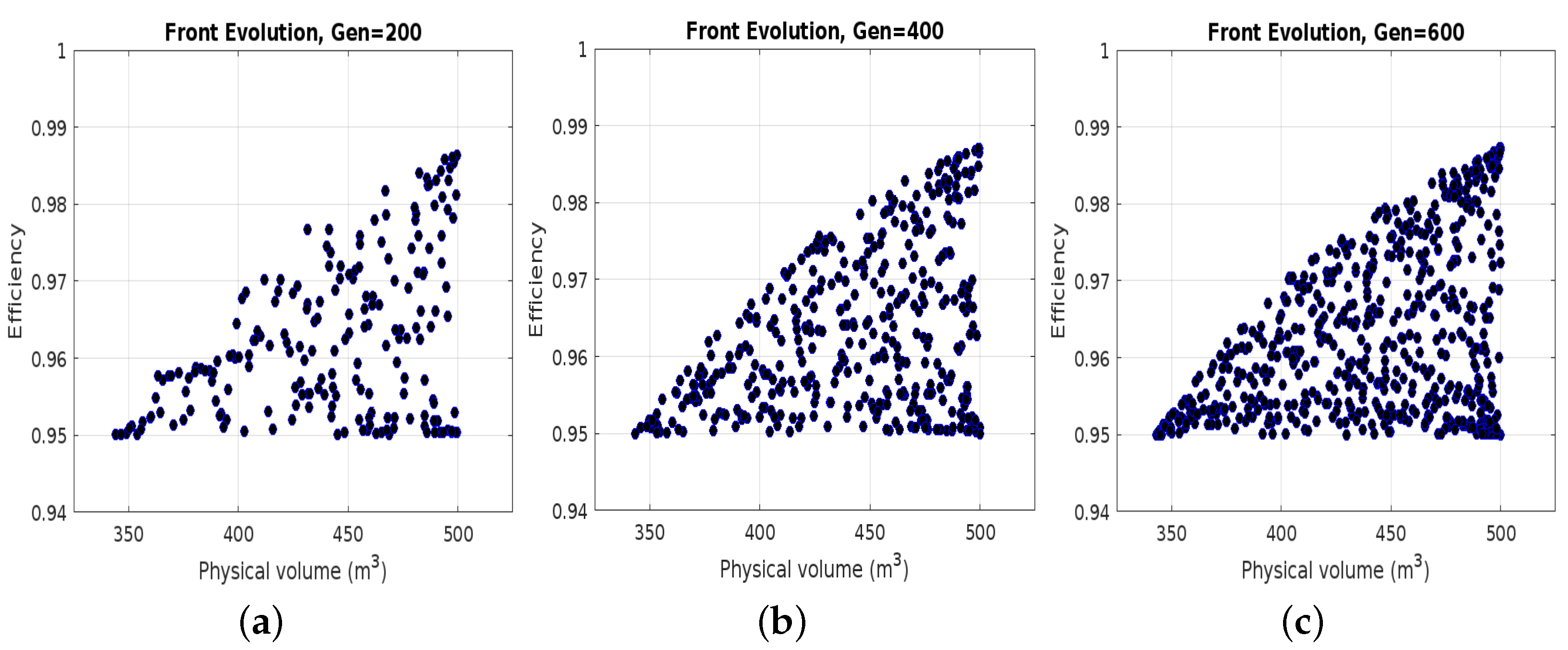
The Pareto front is generated by post-processing all data generated by the evolutionary optimizer using Matlab Online [20], based on the confrontation of objectives with population and generation values at 200, 400 and 600, respectively. In this sense, given a vector of design variables, x is said to be dominated over by other vector of design variables y if
Otherwise, x is said to be a Pareto front if x is non-dominated by any other vector of design variables z ∈ X such that [14]. In this way, Figure 2a shows that with a lower number of population and generation, there is greater dispersion of the solutions. Increasing P and G, a higher population density is obtained and results in a better observation of the behavior of the non-dominated solutions and the Pareto front as illustrated in Figure 2b,c. Here, each blue point represents an acceptable design for HFSW that satisfies the constraints.
Figure 3 shows the ideal Pareto front vs. the found Pareto front, where P = G = 600 are used. Clearly, Figure 3 shows a min–max problem, and all individuals of the population are in the search space with the constraints above defined. Therefore, all solutions are valid. Additionally, any blue point in Figure 3 (right side) can be selected, and the numerical value of each design variable can automatically be obtained. But also, all the found solutions can be stored in a database in order to be used in a next process, saving CPU resources.
In this sense, and selecting a solution point on the Pareto front of Figure 3 (right side), the design of the HFSW is represented in Figure 4. From this solution, we obtain = 0.968 (equivalent to > 96.8%), = 401.445 m3, where the numerical values of each design variable for the construction of HFSW are t = 13.122 d, W = 27.446 m, L = 74.869 m, = 0.1 m, = 2 m and s = 0.556% as given in the penultimate row of Table 2. The results indicate that the NSGA-II algorithm, adapted to the specific characteristics of wetlands, manages to generate solutions that optimize the efficiency of wastewater treatment, which supports its viability and usefulness in wastewater management.
Moreover, we compare the results generated by the proposed methodology associated with an individual of the Pareto front with those designs of HFSW reported in the literature as described in Table 3. It is found that all works are fully custom designs and some of them have small dimensions, limiting the volume capacity in gray-water treatment. Further, all cited references not only do not report the numerical value of the design variable used but also almost all them use a slope equal to 1, and is lower compared to the result obtained with the proposed methodology. Furthermore, it can also be observed that t tends to increase when also increases and, therefore, results in greater volume capacity in gray-water treatment. It is important to mention that, whereas one fully custom design is reported in [4,5,10,12], with the developed methodology, P acceptable designs are generated. For instance, from Figure 2c, we have P = 600 acceptable artificial wetland designs. As a consequence, any physical design represented by a blue point of Figure 3 can be selected, and its design features are much better that those reported in Table 3.
5. Discussion
The use of the NSGA-II algorithm allows us to explore a wide range of solutions and generate the Pareto front. This front not only represents the non-dominated solutions but also offers a clear view of the balance between objective functions. By considering different values of P and G during the optimization process, a better understanding of the behavior of the solutions is provided. Therefore, with high values of P and G, the Pareto front is better formed, providing a valuable tool for decision making since it allows different design options to be evaluated based on specific design variables and constraints. Regarding the established constraints, these can also be evident on the Pareto front since the multi-objective optimization algorithm has identified solutions that exceed the 95% contaminant removal threshold, maintaining the at below 500 m3. This finding demonstrates the effectiveness and ability of the NSGA-II algorithm to optimize the HFSW design. A disadvantage of the proposed HFSW design methodology is that if more objective functions are used along with constraints, the multi-objective optimization process becomes more complex and not only are more CPU resources required but the space of design must also be expanded in order to search for a better combination of all the design variables that satisfy all the objective and constraint functions. As a consequence, more CPU time is required since P and G also must be increased in order to obtain greater diversity. Furthermore, the evolutionary optimizer could also fail since it is limited to using a low number of objective functions. This is another disadvantage since the real design of an HFSW consists of several objective functions, both biological and physical, among others. In this sense, the proposed design methodology can also be used for optimizing the biological part of an HFSW and then merging both Pareto fronts, the one generated for the physical part and for the biological part. As a consequence, it is possible to obtain an acceptable final design of the HFSW. Moreover, because the NSGA-II algorithm is based on genetic algorithms and the crossover and mutation probability indices are usually kept constant throughout the optimization process, it is possible to generate identical individuals between generations. As a consequence, local optimal solutions are found. Note that this last behavior is also due to the fact that NSGA-II is elitist, and the best individuals found in each generation are always kept on the Pareto front. A possible solution to this problem is to randomly change the mutation and crossover probability indices between generations or perhaps combine other optimization algorithms with NSGA-II. These tasks are lines of future work.
6. Conclusions
This research demonstrates that using the NSGA-II algorithm for HFSW management is a promising strategy to address the specific changes associated with these types of ecosystems. It was possible to obtain the best solutions for the vector of design variables and represent the Pareto front and, therefore, at a smaller population size P and fewer generations G of greater dispersion, given that the solution of the design variables for HFSW with the input data P and G has greater dispersion. The solution of design variables, found by the NSGA-II algorithm, depends on the values of P and G, the constraint and objective functions. These results suggest that optimization with the NSGA-II algorithm can play a crucial role in the constructed wetland, providing tools for data-driven decision making and implementing sustainable management practices and strategy to the peculiarities of the HFSW. However, the evolutionary optimizer is limited to using few objective and constraint functions since increasing their number not only increases the complexity of the solution but also increases the use of CPU resources, and the optimizer cannot find acceptable solutions. This is a serious disadvantage since the real design of artificial HSFWs is composed of several physical and biological performance objectives that must be satisfied simultaneously, and this is a conflict that exists among them.
Author Contributions
Conceptualization, J.M.-V. and E.R.-P.; methodology, C.S.-L. and E.R.-P.; software, J.M.-V. and C.S.-L.; validation, J.M.-V., E.R.-P. and C.S.-L.; formal analysis, J.M.-V. and E.R.-P.; investigation, J.M.-V. and E.R.-P.; writing—original draft preparation, J.M.-V. and E.R.-P.; writing—review and editing, C.S.-L.; visualization, J.M.-V.; supervision, E.R.-P. and C.S.-L. All authors have read and agreed to the published version of the manuscript.
Funding
This research received no external funding.
Institutional Review Board Statement
Not applicable.
Informed Consent Statement
Not applicable.
Data Availability Statement
Data are contained within the article.
Acknowledgments
The first author thanks CONAHCyT 1240559 Master Grant.
Conflicts of Interest
The authors declare no conflicts of interest.
References
- Stefanakis, A.I. The Role of Constructed Wetlands as Green Infrastructure for Sustainable Urban Water Management. Sustainability 2019, 11, 6981. [Google Scholar] [CrossRef]
- Choudhary, A.K.; Kumar, P. Constructed Wetland: A Green Technology for Wastewater Treatment. In Environmental Microbiology and Biotechnology: Volume 1: Biovalorization of Solid Wastes and Wastewater Treatment; Singh, A., Srivastava, S., Rathore, D., Pant, D., Eds.; Springer: Singapore, 2020; pp. 335–363. [Google Scholar] [CrossRef]
- Cheng, H.; Kim, S.; Hyun, J.H.; Choi, J.; Cho, Y.; Park, C. A multi-objective spatial optimization of wetland for Sponge City in the plain, China. Ecol. Eng. 2024, 198, 107147. [Google Scholar] [CrossRef]
- Fonseca-Castro, M. Diseño de Humedal Construido para Tratar los Lixiviados del Proyecto de Relleno Sanitario de Pococí; 2010. Available online: https://repositoriotec.tec.ac.cr/handle/2238/6158 (accessed on 17 February 2024).
- Núñez Burga, R.M.F. Tratamiento de Aguas Residuales Domésticas a Nivel Familiar, con Humedales Artificiales de flujo Subsuperficial Horizontal, Mediante la Especie Macrófita Emergente Cyperus Papyrus (Papiro). 2016. Available online: https://repositorio.upeu.edu.pe/handle/20.500.12840/555 (accessed on 17 February 2024).
- Konak, A.; Coit, D.W.; Smith, A.E. Multi-objective optimization using genetic algorithms: A tutorial. Reliab. Eng. Syst. Saf. 2006, 91, 992–1007. [Google Scholar] [CrossRef]
- Yusoff, Y.; Ngadiman, M.S.; Zain, A.M. Overview of NSGA-II for Optimizing Machining Process Parameters. Procedia Eng. 2011, 15, 3978–3983. [Google Scholar] [CrossRef]
- Ikenberry, C.; Darling, J.; Talley, C.; Williams, J.; McPeak, J.; Gilmore, S.; Steck, D.; LaFreniere, L.; Ruhge, T. A Multi-Objective Water Quality Wetland to Complement Phytoremediation of Contaminated Groundwater. In Proceedings of the World Environmental and Water Resource Congress 2006, Omaha, Nebraska, 21–25 May 2006; pp. 1–11. [Google Scholar] [CrossRef]
- Huang, J.J.; Gao, X.; Balch, G.; Wootton, B.; Jørgensen, S.E.; Anderson, B. Modelling of vertical subsurface flow constructed wetlands for treatment of domestic sewage and stormwater runoff by subwet 2.0. Ecol. Eng. 2015, 74, 8–12. [Google Scholar] [CrossRef]
- Andreo-Martínez, P.; García-Martínez, N.; Almela, L. Domestic Wastewater Depuration Using a Horizontal Subsurface Flow Constructed Wetland and Theoretical Surface Optimization: A Case Study under Dry Mediterranean Climate. Water 2016, 8, 434. [Google Scholar] [CrossRef]
- Liao, R.; Jin, Z.; Chen, M.; Li, S. An integrated approach for enhancing the overall performance of constructed wetlands in urban areas. Water Res. 2020, 187, 116443. [Google Scholar] [CrossRef]
- López-Linares, E.; Rodríguez-Álvarez, M. Evaluación de un Humedal Artificial de Flujo Subsuperficial Como Tratamiento de Agua Residual Doméstica en la Vereda Bajos de Yerbabuena en el Municipio de Chía, Cundinamarca. Master’s Thesis, Instituto Tecnológico de Costa Rica Escuela de Ingeniería en Construcción, Costa Rica, Universidad de la Salle Facultad de Ingeniería Ambiental y Sanitaria, Bogotá, Colombia, 2016. [Google Scholar]
- Dotro, G.; Langergraber, G.; Molle, P.; Nivala, J.; Puigagut, J.; Stein, O.; Von Sperling, M. Humedales para Tratamiento; Biological Wastewater Treatment Series; IWA Publishing: London UK, 2021. [Google Scholar]
- Farid, M.; Lim, H.S.; Lee, C.P.; Latip, R. Scheduling Scientific Workflow in Multi-Cloud: A Multi-Objective Minimum Weight Optimization Decision-Making Approach. Symmetry 2023, 15, 2047. [Google Scholar] [CrossRef]
- Corporación Centro de Investigación en Palma de Aceite; Gonzalez, A.; Rodríguez, N.; García, A.; Ruiz, E.; Acero, J. Humedales Artificiales Como Alternativa para el Tratamiento Terciario de Efluentes de Planta de Beneficio de Palma de Aceite. 2022. Available online: https://repositorio.fedepalma.org/handle/123456789/141561 (accessed on 17 February 2024).
- CONAGUA. Manual de Agua Potable, Alcantarillado y Saneamiento Diseño de Plantas de Tratamiento de Aguas Residuales Municipales: Zonas Rurales, Periurbanas y Desarrollos Ecoturísticos. Available online: https://agua.org.mx/biblioteca/manual-de-agua-potable-alcantarillado-y-saneamiento/ (accessed on 17 February 2024).
- Val del Río, Á.; Campos Gómez, J.; Mosquera Corral, A. Technologies for the Treatment and Recovery of Nutrients from Industrial Wastewater; Advances in Environmental Engineering and Green Technologies (2326-9162); IGI Global: Hershey, PA, USA, 2016. [Google Scholar]
- Deb, K. Multi-Objective Optimization Using Evolutionary Algorithms; Wiley Interscience Series in Systems and Optimization; Wiley: New York, NY, USA, 2001. [Google Scholar]
- Deb, K.; Pratap, A.; Agarwal, S.; Meyarivan, T. A fast and elitist multiobjective genetic algorithm: NSGA-II. IEEE Trans. Evol. Comput. 2002, 6, 182–197. [Google Scholar] [CrossRef]
- MathWorks®. Matlab Online. 2024. Available online: https://la.mathworks.com/products/matlab-online.html (accessed on 17 February 2024).
Figure 1.
NSGA-II algorithm flowchart [19].
Figure 1.
NSGA-II algorithm flowchart [19].

Figure 2.
Dispersion in Pareto front: (a) P = 200, (b) P = 400 and (c) P = 600.

Figure 3.
Ideal Pareto front (left side) vs. found Pareto front (right side).
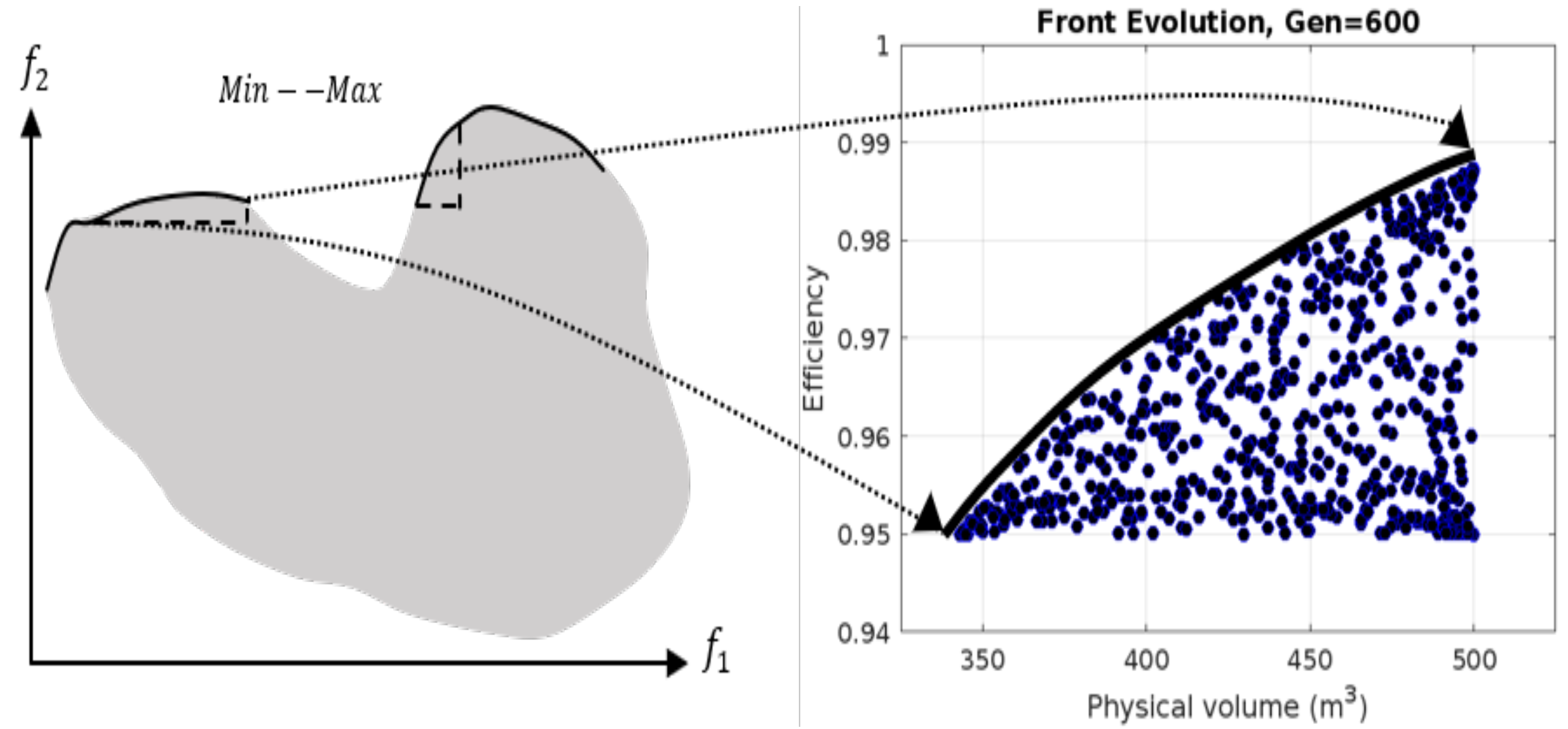
Figure 4.
Scheme of the design of the HFSW.


Table 1.
Design variables.
| Design Variable | Literature | This Work | Units |
|---|---|---|---|
| t | 4–15 1, 2–7 2,3 | 1–60 | d |
| W | 1–61 2 | 20–100 | m |
| L | 1–15 2 | 20–100 | m |
| 0.46–0.76 1, 0.5–0.6 2 | 0.7–10 | m | |
| 0.061–0.3 1, 0.4–0.5 2 | 0.1–0.8 | m | |
| s | 0.5–1 1 | 0–1 | % |
Table 2.
Set of solutions found for different P and G values.
| Objectives | Design Variables | Constraints | ||||||||||
|---|---|---|---|---|---|---|---|---|---|---|---|---|
| P | G | t | W | L | s | (7) | (8) | (9) | ||||
| 200 | 200 | 0.986 | 497.249 | 16.371 | 57.690 | 85.842 | 0.121 | 1.983 | 0.205 | 0.036 | 2.751 | 87.228 |
| 0.960 | 445.689 | 12.249 | 58.355 | 91.402 | 0.125 | 1.993 | 0.241 | 0.010 | 54.311 | 83.664 | ||
| 0.952 | 365.519 | 11.551 | 57.281 | 89.345 | 0.125 | 1.972 | 0.209 | 0.002 | 134.481 | 82.499 | ||
| 0.954 | 415.011 | 11.715 | 58.005 | 84.922 | 0.128 | 1.939 | 0.208 | 0.004 | 84.989 | 89.092 | ||
| 400 | 400 | 0.964 | 420.480 | 12.671 | 75.585 | 91.314 | 0.102 | 1.999 | 0.258 | 0.013 | 79.520 | 135.442 |
| 0.983 | 484.063 | 15.568 | 70.908 | 86.127 | 0.101 | 1.998 | 0.249 | 0.033 | 15.937 | 126.599 | ||
| 0.952 | 399.941 | 11.602 | 71.475 | 87.568 | 0.103 | 1.925 | 0.266 | 0.002 | 100.059 | 126.857 | ||
| 0.958 | 401.298 | 12.125 | 73.624 | 89.531 | 0.101 | 2.000 | 0.265 | 0.008 | 98.702 | 131.339 | ||
| 600 | 600 | 0.970 | 448.090 | 13.357 | 30.290 | 78.446 | 0.100 | 2.000 | 0.574 | 0.020 | 51.911 | 12.423 |
| 0.957 | 489.734 | 12.036 | 35.909 | 77.218 | 0.100 | 1.998 | 0.582 | 0.007 | 10.266 | 30.508 | ||
| 0.968 | 401.445 | 13.122 | 27.446 | 74.869 | 0.100 | 2.000 | 0.556 | 0.018 | 98.555 | 7.468 | ||
| 0.970 | 422.962 | 13.384 | 26.367 | 74.646 | 0.101 | 2.000 | 0.589 | 0.020 | 77.038 | 4.455 | ||
Disclaimer/Publisher’s Note: The statements, opinions and data contained in all publications are solely those of the individual author(s) and contributor(s) and not of MDPI and/or the editor(s). MDPI and/or the editor(s) disclaim responsibility for any injury to people or property resulting from any ideas, methods, instructions or products referred to in the content. |
© 2024 by the authors. Licensee MDPI, Basel, Switzerland. This article is an open access article distributed under the terms and conditions of the Creative Commons Attribution (CC BY) license (https://creativecommons.org/licenses/by/4.0/).
Share and Cite
MDPI and ACS Style
Mendez-Valencia, J.; Sánchez-López, C.; Reyes-Pérez, E. Multi-Objective Design of a Horizontal Flow Subsurface Wetland. Water 2024, 16, 1253. https://doi.org/10.3390/w16091253
AMA Style
Mendez-Valencia J, Sánchez-López C, Reyes-Pérez E. Multi-Objective Design of a Horizontal Flow Subsurface Wetland. Water. 2024; 16(9):1253. https://doi.org/10.3390/w16091253
Chicago/Turabian StyleMendez-Valencia, Jhonatan, Carlos Sánchez-López, and Eneida Reyes-Pérez. 2024. "Multi-Objective Design of a Horizontal Flow Subsurface Wetland" Water 16, no. 9: 1253. https://doi.org/10.3390/w16091253
Note that from the first issue of 2016, this journal uses article numbers instead of page numbers. See further details here.