
Groundwater Chemical Trends Analyses in the Piedmont Po Plain (NW Italy): Comparison with Groundwater Level Variations (2000–2020)


Earth Sciences Department, University of Turin, Via Valperga Caluso 35, 10125 Turin, Italy
*
Authors to whom correspondence should be addressed.
Water 2024, 16(9), 1240; https://doi.org/10.3390/w16091240
Submission received: 14 March 2024
/
Revised: 16 April 2024
/
Accepted: 24 April 2024
/
Published: 26 April 2024
(This article belongs to the Section Hydrogeology)
Abstract
:The concentrations of chemicals in the groundwater chemical values in the Piedmont Po Plain (NW Italy) show significant temporal variability and need to be characterised due to the lack of regional-scale assessments. The aim of this study was to analyse the trends (period 2000–2020) in the main physicochemical parameters and main ions in 227 wells in the shallow aquifer and to identify the potential causes. The identification of change points (points of sudden change) and comparisons with groundwater level variations were also performed. Results highlight general increasing trends for Na, Cl and HCO3, decreasing trends for SO4 and NO3, stationary conditions for pH and heterogeneous behaviours for electrolytic conductivity, Ca and Mg. Change points occurred in at least 50% of the monitoring wells, mainly during the 2008–2011 period. The comparison between groundwater levels and chemistry highlights a direct proportionality. Superimposed processes that induce an absence of proportionality are shown. The comparison of results with those of previous studies conducted under similar conditions revealed similar variations.. In conclusion, the potential responsible factors (e.g., road-salt dissolution and agricultural practices) and the relevant role of groundwater level variation were identified.
1. Introduction
The global interest in the variability of groundwater quality is growing, and researchers are interested in identifying factors that can deteriorate groundwater resources [1]. The physicochemical parameters are characterised by different sources that influence their values, and at the same time, several processes normally affect the physicochemical values of groundwater [1]. Previous studies have confirmed the relevant role of natural processes, such as climate change [2,3], geological features [4], microbiological features [5] and anthropogenic processes [6], in modifying groundwater quality. The impacts of climate change have been extensively addressed [7,8,9,10,11,12]. Droughts tend to amplify extreme nitrate concentrations, as widely observed in European rivers and groundwater [13,14], and generally, increase ion concentrations with progressive deterioration of water quality [15,16]. Additionally, the increase in groundwater temperatures in the Piedmont Plain [17,18] could influence groundwater chemistry [19]. Therefore, the different responses of aquifers to climate change result in different resilience capacities [20]. A number of documented global groundwater contaminant challenges related to the use of large quantities of agrochemical components have been reported for anthropogenic processes. The anthropogenic pressures influencing the groundwater chemistry are countless [6]. In particular, extensive irrigation represents a relevant recharge that can induce the dilution or concentration of NO3. In particular, a dilution of NO3 in groundwater in the Lombardy Plain occurred [21]. However, a worsening of groundwater quality can occur due to irrigation practices [22,23,24,25]. Irrigation return flow has a negative impact on groundwater quality, promoting the leaching of fertilisers from agricultural soils to aquifers and generating groundwater with high concentrations of NO3 [26]. At the same time, urbanisation also induces variations (e.g., road-salt application and accumulation in the environment) [27,28]. Another process that could control groundwater chemistry is interaction with the watercourses [29,30,31]. Surface water and groundwater are often treated as separate entities. However, almost all surface water continuously interacts with shallow groundwater, and the contamination of one environmental matrix can be reflected by the other matrix. Additionally, groundwater salinisation trends are usually evaluated in arid areas [32,33]. Various mountain spring studies have been conducted on karst systems [34,35,36], highlighting that local hydrogeological conditions, land-use features and climate change influence spatiotemporal groundwater quality.
Considering the presence of plain aquifers in Europe, several studies analysing long-term trends and change points, in particular, have been conducted [37,38,39], with greater interest in NO3, intensive agricultural practices and the effectiveness of regulated limitations [40,41,42,43,44,45,46,47,48]. Some studies compare the groundwater level and chemistry, revealing proportionalities [49,50]. Additionally, in the Italian context, studies have been conducted in recent years, mainly at the local scale [51,52,53,54].
The groundwater quality in the Piedmont Po Plain (NW Italy) shows a relevant temporal variability that is necessary to characterise due to the lack of a regional-scale assessment. Several studies have been conducted only at the local scale [55,56,57,58,59,60], and even fewer have been conducted in the alpine context [61,62].
However, knowing what happened in the past is fundamental to understanding the processes that took place, enabling us to influence future conditions and guide us to the correct choices we will have to make. The aim of this study was to analyse the trends (period 2000–2020) of the main physicochemical parameters (EC (electrolytic conductivity), pH, HCO3, NO3, SO4, Ca, Mg, Na and Cl) in 227 monitoring wells in the shallow aquifer of the Piedmont Po Plain and to identify the potential causes. At the same time, the identification of change points and comparisons with groundwater level variations were performed.
2. Materials and Methods
2.1. Study Area
2.1.1. Geological and Hydrogeological Setting
The study area is located in the Piedmont region in northwestern Italy (Figure 1). From a geological and geomorphological point of view, the Piedmont region can be divided into three macrosectors: the Alps–Apennine chains, the hilly sector and the plain sector. The Piedmont Plain extends approximately 6230 km2, equal to 27% of the region, and represents the westernmost part of the Po Plain [63]. The geological settings of the Piedmont Alps and Apennines are highly variable and widely investigated. From a lithological point of view, calcareous and dolomitic rocks and evaporitic-carbonatic layers, characterised by karst phenomena and metamorphic, volcanic and plutonic rocks, can be distinguished [64]. Alpine crystalline rocks are mostly impermeable or slightly permeable by fissuration. In the hilly sectors, sedimentary rocks, especially marl, clay, silt, conglomerate, sandstone and gypsum, represent the Tertiary Piedmont Basin, which includes the Langhe, Turin and Monferrato Hill deposits. These rocks have low permeability and show limited groundwater circulation.
With regard to the hydrogeological setting, the Piedmont Po Plain consists of various complexes corresponding to the fluvial deposits complex (Lower Pleistocene–Holocene), Villafranchian transitional complex (Upper Pliocene–Lower Pleistocene) and marine complex (Pliocene–Eocene) (Figure 2).
More specifically, Ref. [63] recognised two different hydrogeological complexes hosting shallow unconfined aquifers in the Piedmont plain, with overall thicknesses ranging between 20 and 50 m. In order from youngest to oldest, these complexes consist of the following:
- Recent fluvial deposits (FS1) (Upper Pleistocene–Holocene): fluvial (Holocene) and fluvioglacial (Upper Pleistocene) deposits, mainly gravelly sandy but also silty-clayey. These deposits are located in the bottom of the valleys and in the plain with a prevalent permeability for porosity ranging from high to medium.
- Medium and ancient fluvial deposits (FS2) (Middle–Lower Pleistocene): mainly composed of gravelly sandy and silty-clay deposits. These deposits border the Apennine–Alps chains and are in contact with morainic glacial deposits. A prevalent permeability of medium grade linked to porosity appears, with a lower degree of permeability occurring mainly in the oldest and altered terms. A shallow unconfined aquifer, locally confined, is present in continuity with the aquifer hosted in the FS1 complex.
These complexes, representing Quaternary alluvial deposits, host shallow unconfined aquifers, while the Villafranchian transitional complex (V) and the Pliocene marine sands complex (MS) include confined and semiconfined aquifers, representing deep aquifers.
The water table follows the topography of the land surface, and the piezometric lines are generally parallel to the Alps relief (Figure 3). The main watercourses are generally losing rivers close to the Alps and gaining rivers in the low plain. The water table depth shows high variability. The most frequent range is less than 5 m, while the highest values (more than 50 m) are found on high morphological terraces. The recharge areas of the shallow aquifers are located across the entire plain due to infiltration from rainfall and surface waters in the high plain sectors. The low plain sectors are discharge areas, and the Po River constitutes the main regional discharge axis for groundwater flow [63].
2.1.2. Hydrochemical and Land-Use Setting
In terms of the hydrochemical setting, several local studies have investigated the groundwater quality in the Po Plain, with a large number of local studies [54,65,66,67].
Overall, at the regional level, the spatial distribution of the concentrations shows areal differences between sectors. The Biella–Vercelli–Novara Plains had lower concentrations than did the southern sectors of the study area. For EC, HCO3, SO4, Ca and Mg, the Asti sector had the highest values; the Cuneo and Alessandria Plains had higher values than did the Biella–Vercelli–Novara Plains and a portion of the Torino Plain. Na and Cl showed the highest concentrations in the Asti sector, followed by those in the Alessandria Plain and Poirino Plateau (mainly above 20 mg/L). Concentrations below 20 mg/L were detected in the Cuneo Plain, Torino Plain and Biella–Vercelli–Novara Plains. NO3 shows the highest concentrations in the Cuneo Plain, Alessandria Plain and Poirino Plateau and, to some extent, in the Torino Plain (mainly above 20 mg/L). Concentrations less than 20 mg/L were detected in the Asti sector and Biella–Vercelli–Novara Plains. The pH was essentially in neutral values (6.5–7.5), with lower values (more acid) in the Pinerolo Plain and the upper Biella–Vercelli–Novara Plains [68].
Some previous studies have been conducted to evaluate the temporal evolution of hydrochemical characteristics [57,60,69], while others have characterised the high nitrate contamination linked to intense agricultural activities [65,70,71]. The designation of nitrate-vulnerable zones (ZVN) of agricultural origin has evolved over time in the Piedmont Plain, with designation of new areas in 2002, 2006, 2008, 2019 and 2020, corresponding to 47% of the entire regional agricultural area [72]. In the study area, irrigated arable areas are prevalent, except in the Vercelli–Novara Plains, where paddies are widely present. The main industrial areas are located close to large urban centres [73].
2.2. Materials and Methods
In this paper, 74,013 pieces of groundwater chemical data from 227 shallow aquifer wells in the Piedmont Po Plain were analysed (Figure 4). Physicochemical data were obtained from sampling campaigns performed by the ARPA Piemonte (Regional Agency for Environmental Protection), which consisted of half-yearly sampling for the period 2000–2020 (21 years) (spring and autumn seasons, with two samples every year in the better condition of completeness). The first sampling took place between February and June, while the second took place between September and December. The physicochemical data are freely available at the ARPA Piemonte website [74]. The groundwater sampling and hydrochemical analyses were conducted by the ARPA Piemonte in compliance with the European Directives [75,76,77].
The main physicochemical parameters (EC, pH, HCO3, NO3, SO4, Ca, Mg, Na and Cl) of the shallow aquifer were selected due to the greater availability of data compared to other ions and the deep aquifer. K was not analysed due to the high number of values below the detection limit. The ARPA Piemonte conducted sampling campaigns on more than 600 different wells/piezometers that captured the shallow aquifer since the beginning of the monitoring activities. The selected monitoring wells correspond to those with a completeness of at least 80% for EC (% half-yearly chemical data available for the overall period). A total of 34 monitoring points with a completeness between 70 and 80% were added in relation to the characterisation of the groundwater level already performed in a previous study [56]. The average completeness values were 94% for EC, SO4, NO3, Cl and pH and 61% for Na, HCO3, Ca and Mg.
The nonparametric Mann‒Kendall trend test [78,79] was applied to detect the existence of statistically significant positive or negative monotonic trends in the physicochemical parameter temporal series, and the ordinary least squares (OLS) regression slope was used to quantify the magnitude of the trends. The Mann‒Kendall statistic test (S) was applied as indicated below:
An increasing trend is detected when a positive value of S emerges, while a negative value indicates a decreasing trend. The data show a statistically significant trend in the case of the rejection of the null hypothesis H0 at the level of significance α (0.05) [80]. With respect to the significance of the Mann‒Kendall test, approximately 40 pieces of data are needed; however, for a rough estimate, the minimum number of pieces of data is 10 [80]. OLS regression is typically used to determine linear relationships between a dependent response variable and one or more predictor (independent) variables [81]; however, statistical inference on the slope of the OLS line can also be used to determine trends in the time-series data used to estimate an OLS line. The trends and OLS analyses in each monitoring well for the physicochemical parameters (EC, pH, HCO3, Ca, Mg, Na, NO3, Cl and SO4) were performed with the software ProUCL 5.1 [82], with a confidence level of 95%. Considering the absence of clear seasonal fluctuations and the amount of data, the trend analyses were performed on the entire time series, deeming them inappropriate for defining trends in the spring and autumn season series. The main elaborations created for trend analyses were related to the spatialisation of the temporal results to highlight potentially different temporal responses between sectors.
Change-point analysis (ChPA) is a statistical test able to detect sudden and maintained changes (change points (ChPs)) in the time series. This test allows us to determine whether and when a variation has taken place and to divide the series into subperiods characterised by homogeneous parameter behaviours. ChPA was performed through the statistical nonparametric Pettitt test [83]. This test is calculated according to:
where T is the number of pieces of data in the time series, Xi and Xj are the data values at times i and j (with j > i), respectively, and sgn (Xi − Xj) is the sign function. For the t value (instant of the series), a value of U(t, T) is detected and reported. The analysis of the diagram of the function U(t, T) makes it possible to identify the moment at which a change point occurred. The maximum or minimum point of the function U(t, T) highlights the moment in which a change point occurs if the test result was such that the null hypothesis H0 was rejectable at the assigned significance level. In this study, to confirm the detection of a significant change, a 95% confidence interval was needed, with a level of significance α of 0.05. ChPA was performed through the ANABASI program version 1.51 beta, a statistical tool developed by ISPRA [84]. For the ChPA, only data time-series with high completeness, and therefore continuity, can be investigated. For this reason, identification was performed only for EC, NO3, SO4 and Cl. Because potential multiple ChPs could exist in individual monitoring wells, for this temporal characterisation, only the main ChP for each monitoring well was detected; indeed, the small amount of data constituting the time series did not make it possible to break the series. Following the identification of the ChPs, it is possible to recognise two segments on which, theoretically, it is possible to carry out trend analysis. However, this analysis is only reliable with large amounts of data. For this reason, the trends of the splits were not analysed. ChPA aims to detect whether there is any change in the sequence of time series and, when it occurs, to evaluate the number of changes and their corresponding locations in time (semesters of occurrence) for physicochemical parameters.
As concerns the comparison between groundwater chemistry and groundwater levels, 34 monitoring wells already selected by [56] were investigated. The selection of the same monitoring wells was dictated by the decision not to repeat the numerous phases already addressed, such as the numerous elaborations and comparisons carried out, primarily with rainfall. Since 2000, the monitoring wells have composed the automatic monitoring network of the ARPA Piemonte. Daily groundwater level data are available on the website of the ARPA Piemonte [74]. The data were aggregated monthly, and the monthly average of groundwater levels were obtained.
In this study, trends and change-point results were compared with groundwater chemistry results. Furthermore, visual comparisons between the groundwater levels and groundwater chemistry time-series were performed to identify the predominant transport mechanism of ions in solution between dilution (a decrease in physicochemical values with increasing groundwater level) or the transfer of substances contained in the vadose zone, which are mobilised by groundwater level variation (an increase in physicochemical values with increasing groundwater level). Moreover, the evaluation of potential differences between the time series could lead to a better understanding of the existing processes.
Moreover, the evidence from previous studies conducted in a similar hydrogeological and climatic context or in areas close to this one was considered and compared. The same time periods between previous studies and this study were not considered mandatory for comparison due to the evaluation of the processes responsible for the temporal evolution.
3. Results
The trend analysis results are summarised in Table 1 and Table S1 of the Supplementary Material. Trend analysis reveals different results and behaviours between parameters. At the regional level, the presence of trends (the sum of monitoring points with increasing or decreasing trends) appears prevalent, or substantially equivalent, with respect to the monitoring points with an absence of trends, appearing for EC, Mg, Na, Cl, NO3 and SO4. More specifically, considering the individual trends result (increasing, decreasing or no trend), Na and SO4 show prevalent increasing and decreasing trends, respectively, while the other physicochemical parameters show a prevalent absence of trends. Excluding points with no trends and comparing the increasing and decreasing trends for the remaining points, EC, HCO3, Ca, Na, Cl and Mg clearly show more increasing trends than decreasing trends, while the opposite situation exists for NO3, SO4 and pH.
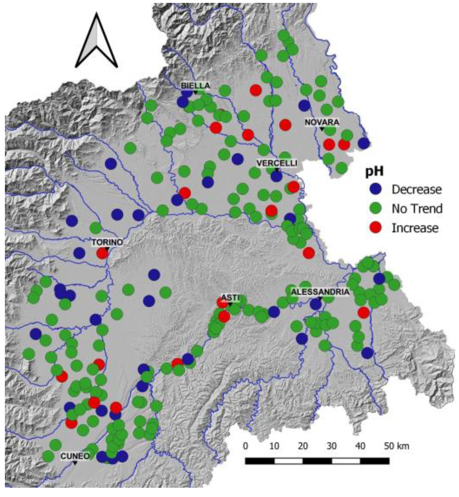
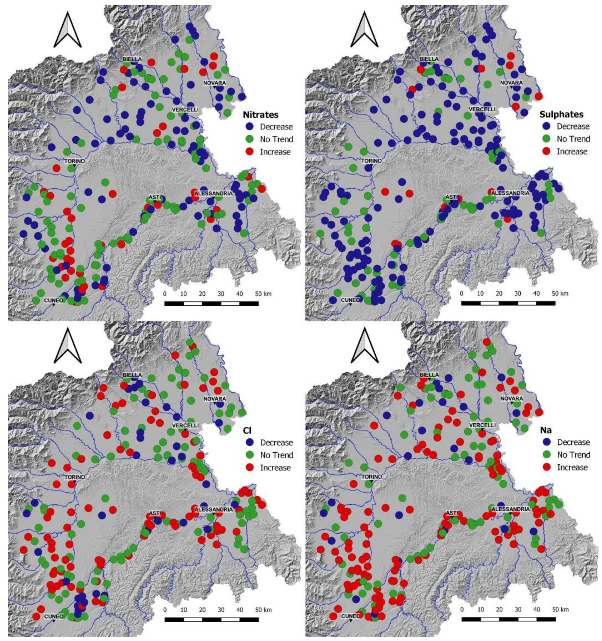
The spatial representations of the trend results (Figure 5, Figure 6 and Figure 7) do not show regular spatial trends, with numerous cases of opposite trends between the monitoring wells closest to each other. At the same time, however, it is possible to appreciate sectors with homogenous trends within them. For example, EC shows local areas with increasing trends along the Maira River (Cuneo Plain) and the Sale–Tortona area (Alessandria Plain). In the plain portion closest to the Alps in the Cuneo and Torino plains, decreasing trends and no trends for HCO3, Mg and NO3 are present. NO3 shows increasing trends mainly in the central Cuneo Plain and in the Biella and Novara terraces. Decreasing trends of Na and Cl are highlighted mainly in the Biella and Vercelli plains. At the same time, however, other very local clusters constituted by few monitoring wells closest to each other are visible.
The magnitude of the trends at the regional level are expressed as mg/L variation over time and as % variation over time; the latter is compared to the average value detected over 21 years, and the results are summarised in Table 2. The magnitude of trends expressed as mg/L (or μS/cm) variations is directly proportional to the average concentrations for all the physicochemical parameters. EC, Cl, Na, SO4 and pH show greater variations with increasing trends than with decreasing trends. The opposite situation was observed for the other ions (HCO3, Ca, Mg and NO3). The magnitude expressed as % variations shows no proportionality with average concentrations, with only a partial inverse proportionality for NO3 and HCO3. EC, HCO3, Ca, Mg and pH show average % variations below 35%, while NO3, Cl, Na and SO4 mainly exceed 40%. The % variations in the decreasing trends were greater than those in the increasing trends, except for SO4 and pH.
In terms of spatial distribution, NO3 showed the greatest variations in the Cuneo, Alessandria and Biella plains with particular homogenisation in the Vercelli and Novara plains characterised by low variations. SO4, Na, Cl, Ca and Mg show the highest values mainly in the Asti sector and Alessandria Plain, followed by the other sectors.
ChPs were detected in at least 50% of the monitoring wells (52% EC, 58% NO3, 66% Cl and 81% SO4) (Table S2 of the Supplementary Material). A comparison of the first and second sampling campaigns (spring and autumn, respectively) revealed that Cl and NO3 were more abundant in the spring season than in the autumn season, while EC and SO4 were more abundant in the autumn season (Figure 8); 50% of ChPs occurred in the 2008–2011 period (75% for SO4), mainly in 2009 (Figure 9). The presence of peaks of high concentrations induced uncertainties regarding the identification of ChPs, causing the exclusion of 7 points for EC and 1 point for NO3. The spatial distributions of ChPs are not regular; however, it is possible to recognise some local clusters with the same or similar ChP moment. Taking a look at the behaviour of concentration after ChPs, a decrease in concentration was mainly detected for SO4, while NO3 showed increasing concentrations in the Cuneo and Pinerolo plains and decreasing concentrations in the other sectors, mainly. The comparison between chemical parameters reveals that only 10% of monitoring wells highlight the same time moment of occurrence of ChP.
As reported in [56], a negative groundwater level trend in 2002–2008 and 2009–2017 was defined, highlighting a similar behaviour to that of the rainfall series. The visual comparison between the groundwater level and groundwater chemical series highlights several aspects. In the prevalent comparison diagrams, a general direct proportionality appears (Figure 10). In the individual monitoring wells, some but not all physicochemical parameters show a proportionality with groundwater level. Considering all the monitoring wells, all the selected physicochemical parameters occasionally showed a proportionality with the groundwater level; however, the best proportionalities were found for those with complete time series. In some cases, the existence of temporal lag was highlighted. The quantification of the temporal lag reveals a typical delay of 6–12 months and occasionally a delay of 18–24 months (Figure 11). These delays were detected in numerous monitoring wells; however, they lacked a regular spatial distribution. Furthermore, in individual monitoring wells, not all physicochemical parameters showed a temporal lag or the same temporal lag. No regular delays emerged in the comparison of physicochemical parameter delays. Relevant contamination phenomena with a peak increase in concentration without variation in groundwater level were well distinguished.
In some monitoring wells and at specific time moments, there was no response of the physicochemical parameters to groundwater level variation. Furthermore, monitoring wells with clear seasonal fluctuations in groundwater levels sometimes do not show similar chemical variations (Figure 12a,b). The absence of chemical responses can be partially attributed to the specific time moment of sampling activities, which, with only two pieces of data per year, are unable to intercept and show the influence of groundwater level variation. Another particular aspect was the existence of physicochemical trends without groundwater level trends over time (Figure 12c,d). This condition appears only in paddy areas where agricultural pressures cause the absence of trends in the groundwater level over time. The fact that these behaviours are not influenced by groundwater level (previous Figure 11 and Figure 12) confirms the presence of other natural or anthropogenic processes that differ in terms of groundwater level variations and are also influenced by local geological and hydrogeological features that govern groundwater chemistry over time.
4. Discussion
The trend results that have emerged thus far outline a complex picture. Trends were identified and different behaviours between physicochemical parameters emerged. As concerns spatial distributions, local areas characterised by a homogenisation of trend behaviours within them emerge. Some of these areas are probably influenced by local phenomena, such as intensive agricultural activities (e.g., NO3 in the Cuneo Plain) and the low permeability of the unsaturated zone (NO3 in the Biella–Novara fluvial terraces), inducing a homogenisation of trend results within them.
At first glance at the regional level, the similar behaviour detected between Na and Cl (increasing trends) highlights a correlation with their origin, which corresponds mainly to road-salt application to the roadway network in the winter period, with subsequent accumulation and dissolution processes. Meanwhile, NO3 and SO4, which showed mainly decreasing trends, corresponded to the parameters potentially influenced by denitrification processes. These situations suggest the presence of regional processes, which are superimposed by local processes and influenced by local natural or anthropogenic conditions.
ChPA highlights complex conditions where physicochemical parameters partially exhibit the same temporal behaviours. The high number of ChPs in the 2008–2011 period suggests that processes at the regional level exist. Differences between physicochemical parameters after their comparison and in the spatial distributions confirm the different responses of monitoring wells or groups of monitoring wells to a specific process.
A recent study performed on the Piedmont Plain [56] evaluated the temporal variations in rainfall and mean annual groundwater levels for the 2002–2017 period. The presence of ChPs in 2008 was highlighted at more than 80% of the analysed monitoring points. These ChPs correspond to transitions from a strong lowering to a sudden and considerable increase in the groundwater level. The 2008 ChP was also detected in 88% of the rainfall time-series for the Piedmont Plain, confirming the strong relationship between rainfall and groundwater level. This similarity of the ChP occurrences confirms the relation between groundwater chemistry and groundwater level. Furthermore, the presence of chemical ChPs not only in 2008 but also in the two subsequent years suggests the existence of a temporal lag in the chemical response to the groundwater level changes. These temporal lags could be linked to local natural and anthropogenic features, resulting in variable responses at the regional level. However, not all monitoring wells responded with chemical variations to the 2008 groundwater level ChP, confirming local heterogeneity. According to the results, the transfer of substances contained in the vadose zone mobilised by the increase in groundwater level, which induces a direct proportionality of groundwater levels and chemical contents, appears to be the main process of groundwater chemistry variability over time at the regional level. However, the diffuse decreasing trends of groundwater levels, which should lead to decreasing trends in chemical content, cannot explain the regional increasing trends, e.g., those detected for Na and Cl. For this reason, the existence of secondary processes responsible for the specific temporal differences and the different trends between groundwater level and groundwater chemistry were confirmed. Local contamination phenomena were recognised; however, these phenomena cannot explain the entirety of the temporal differences.
The existence of different temporal lags suggests different transport times of the substances to the monitoring wells. Furthermore, the absence of proportionality between groundwater level and chemistry in some of the investigated monitoring wells was also detected. These behaviours suggest different levels of influence that can translate into different degrees of resilience to groundwater level variations. Furthermore, the land uses in the last 20 years have not highlighted any particular changes at the regional level, with only a slight increase in industrial and residential areas close to urban centres.
The evidence that emerged in previous studies conducted in a similar hydrogeological and climatological context or in areas close to this one could be similar to the results that emerged on the Piedmont Plain and could suggest the processes that took place. Previous studies have generally highlighted the heterogenous spatial distribution of temporal trends between monitoring points [38,45]. In particular, simultaneous decreases, increases and no trends were highlighted for a specific physicochemical parameter at different monitoring points, as was also observed in Piedmont. In these conditions, also when the absence of trends was predominant, a “general and prevalent trend” was attributed.
Previous studies conducted in alpine karst systems in the Piedmont region [61] highlighted different trends for the considered ions compared to those detected in this study, confirming the influences of local aspects, such as geological features. A similar trend for Na and Cl were highlighted in [28], where a future increase in Cl concentrations in groundwater was hypothesised to occur due to the progressive accumulation of road salts in the unsaturated zone and subsequent dispersion. Considering the similarities between the study areas, it is plausible to hypothesise that the same process also potentially occurred on the Piedmont Plain.
NO3 trends in previous European studies conducted on plain aquifers highlighted heterogeneous trends, detecting areas with a remarkable decrease (e.g., Denmark and the Netherlands [43,45]) and others with substantial stationarity or increasing trends (e.g., Germany, Ireland and Poland [47,85]). However, in several studies where long time series were analysed, it was possible to appreciate a “bell curve” with initial increasing and subsequent decreasing trends. This trend reversal was attributed to the national regulations and their application in the limitation of nitrogen compounds used in agricultural practices. In fact, the moments of change correspond approximately to when limitations were introduced [41,42,43,45]. In the Piedmont context, therefore, the introduction of similar limitations since 2002 could explain the main decreasing trends detected. In addition, the increasing trends detected on the Cuneo Plain, where relevant contamination remains over time and intensive agricultural pressures still exist, are potentially linked to a not-virtuous application of limitations. The same process could explain the predominant decrease in SO4 on the Piedmont Plain. Specifically, in the Netherlands, a trend reversal similar to that of NO3 was also detected for SO4 [43]. In particular, high NO3 loads trigger the oxidation of organic matter, thereby reducing the NO3 load either completely or partially, depending on the reduction capacity of the aquifer. The acidification reaction of organic matter is neutralised in a carbonatic aquifer by calcite dissolution, resulting in increasing trends for HCO3 and Ca. Furthermore, in the absence of or decrease in organic matter, acidification processes are not strong, but calcite dissolution is still triggered, yielding increasing trends in HCO3. This process is confirmed by observing the trends detected on the Piedmont Plain, where decreases in NO3 and SO4 concentrations over time can be linked to reductions in organic matter dispersion. At the same time, the general increase in HCO3 corresponds to the response of the aquifer to the neutraliser during the acidifying reaction with a progressive increase in the dissolution of the carbonate component. Furthermore, the predominant absence of trends for pH confirms the neutralisation of acidic and basic processes, with the preservation of existing conditions.
It is also necessary to note the presence of similar trends in areas where the limitations of nitrogen compound use in agricultural practices were not officially applied. This could be linked to the regional efficiency of agricultural practices, which are not limited to the vulnerable zone regulated. Furthermore, the increasing temperature of air and groundwater could contribute, to a minimal extent, to the denitrification processes, as suggested by [19].
5. Conclusions
Temporal characterisation through different approaches involves defining the existence of variation over time and identifying the different typologies of variabilities in trying to hypothesise the responsible processes. The trends analysis highlighted a large number of monitoring wells with statistically significant trends; however, there were heterogeneous results between parameters with spatial distribution differences. The trend results suggest, at first glance, the presence of regionally spatialised processes due to the existence of homogeneous trends at the regional level, superimposed by local processes influenced by local natural or anthropogenic conditions. The essentially absent pH trends suggest that the existing processes were not able to strongly modify the groundwater basicity and equilibrium. The high number of change points and regional diffusion in the 2008–2011 period confirm that processes at the regional level existed. The groundwater level change points detected in a previous study in the same years confirmed the influence of groundwater level variation on groundwater chemistry.
The comparison between groundwater chemistry and groundwater level time-series highlights a general direct proportionality. The temporal lag in the chemical response was highlighted, revealing typical delays of 6–12 months and occasionally until 18–24 months. In individual monitoring wells, some but not all physicochemical parameters show a proportionality with groundwater levels.
Despite the uncertainties that have emerged, the transfer of substances contained in the vadose zone appears to be the main process, regionally spatialised, of the groundwater chemistry variability over time, and the existence of different temporal lags suggests different transport times of the substances to the monitoring wells. The existence of secondary processes responsible for the specific temporal differences and the different trends between groundwater level and groundwater chemistry were confirmed. Due to the geological and hydrogeological heterogeneity of the study area, these secondary processes could be extremely local.
The evidence from previous studies conducted in a similar hydrogeological context highlights a common point in the heterogenous spatial distribution of temporal trends between monitoring points, with simultaneous decreases, increases and no trends for a specific physicochemical parameter. In particular, a similar increasing trend for Na and Cl was also highlighted in areas linked to the accumulation of road salt in the unsaturated zone; therefore, it is plausible to assume that the same process also occurred on the Piedmont Plain. Furthermore, NO3 trends in previous European studies have shown heterogeneous trends, occasionally with trend reversals attributed to national regulations and their application in the limitation of nitrogen compounds used in agricultural practices. In the Piedmont context, the introduction of similar limitations since 2002 could explain the prevalent decreasing and local increasing trends, the latter of which are potentially linked to a non-virtuous application of limitations. As highlighted in other European countries, the limitation of nitrogen compounds could explain the predominant decrease in SO4, increase in HCO3 and lack of change in pH observed on the Piedmont Plain.
According to these new findings, groundwater level variations can be considered among the main influencing factors that, through temporal trends and change points, influence groundwater chemistry over time. At the same time, the presence of superimposed regional and local processes that induce heterogeneous behaviours was confirmed.
In conclusion, this study represents one of the first regional studies on groundwater in which the physicochemical trends, the potential factors responsible and the relevant role of groundwater level variation are analysed, constituting a useful tool for local authorities to increase the effectiveness of environmental protection in a changing global context.
Supplementary Materials
The following supporting information can be downloaded at https://www.mdpi.com/article/10.3390/w16091240/s1: Table S1: Mann–Kendall trend test results; Table S2: Pettitt change-point test results.
Author Contributions
Conceptualisation, D.C., M.L. and D.A.D.L.; methodology, D.C., M.L. and D.A.D.L.; software, D.C.; validation, D.C., M.L. and D.A.D.L.; formal analysis, D.C., M.L. and D.A.D.L.; investigation, D.C.; resources, M.L. and D.A.D.L.; data curation, D.C.; writing—original draft preparation, D.C.; writing—review and editing, D.C., M.L. and D.A.D.L.; visualisation, D.C.; supervision, M.L. and D.A.D.L. All authors have read and agreed to the published version of the manuscript.
Funding
This research received no external funding.
Data Availability Statement
Data are contained within the article and Supplementary Materials.
Conflicts of Interest
The authors declare no conflicts of interest.
References
- Lapworth, D.J.; Lopez, B.; Laabs, V.; Kozel, R.; Wolter, R.; Ward, R.; Amelin, E.V.; Besien, T.; Claessens, J.; Delloye, F.; et al. Devoloping a groundwater watch list for substances of emerging concern: A European perspective. Environ. Res. Lett. 2019, 14, 035004. [Google Scholar] [CrossRef]
- Dao, P.U.; Heuzard, A.G.; Le, T.X.H.; Zhao, J.; Yin, R.; Shang, C.; Fan, C. The impacts of climate change on groundwater quality: A review. Sci. Total Environ. 2024, 912, 16924. [Google Scholar] [CrossRef] [PubMed]
- Earman, S.; Dettinger, M. Potential impacts of climate change on groundwater resources—A global review. J. Water Clim. Chang. 2011, 2, 213–229. [Google Scholar] [CrossRef]
- Vespasiano, G.; Muto, F.; Apollaro, C. Geochemical, Geological and Groundwater Quality Characterization of a Complex Geological Framework: The Case Study of the Coreca Area (Calabria, South Italy). Geosciences 2021, 11, 121. [Google Scholar] [CrossRef]
- Grant, F.F.; Szponar, N.; Edwards, B.A. Groundwater Microbiology; The Groundwater Project: Guelph, ON, Canada, 2021. [Google Scholar]
- Howard, K. Urban Groundwater; The Groundwater Project: Guelph, ON, Canada, 2023. [Google Scholar] [CrossRef]
- Pascoli-Campbell, M.; Reager, J.T.; Hrishikesh, A.C.; Rodell, M. Retracted article: A 10 per cent increase in global land evapotranspiration from 2003 to 2019. Nature 2021, 593, 543–547. [Google Scholar] [CrossRef] [PubMed]
- Stigter, T.Y.; Miller, J.; Chen, J.; Re, V. Groundwater and climate change: Threats and opportunities. Hydrogeol. J. 2023, 31, 7–10. [Google Scholar] [CrossRef]
- Riedel, T.; Weber, T.K.D. Review: The influence of global change on Europe’s water cycle and groundwater recharge. Hydrogeol. J. 2020, 28, 1939–1959. [Google Scholar] [CrossRef]
- Cross, K.; Latorre, C. Which water for which use? Exploring water quality instruments in the context of a changing climate. Aquat. Procedia 2015, 5, 104–110. [Google Scholar] [CrossRef]
- Dragoni, W.; Sukhija, B.S. Climate change and groundwater: A short review. Geolog. Soc. Lond. 2008, 288, 1–12. [Google Scholar] [CrossRef]
- Swain, S.; Taloor, A.K.; Dhal, L.; Sahoo, S.; Al-Ansari, N. Impact of climate change on groundwater hydrology: A comprehensive review and current status of the Indian hydrogeology. Appl. Water Sci. 2022, 12, 120. [Google Scholar] [CrossRef]
- Jutglar, K.; Hellwig, J.; Stoelzle, M.; Lange, J. Post-drought increase in regional-scale groundwater nitrate in southwest Germany. Hydrol. Process. 2021, 35, e14307. [Google Scholar] [CrossRef]
- Saavedra, F.; Musolff, A.; von Freyberg, J.; Merz, R.; Knoller, K.; Muller, C.; Brunner, M.; Tarasova, L. Winter post-droughts amplify extreme nitrate concentrations in German rivers. Environ. Res. Lett. 2024, 19, 024007. [Google Scholar] [CrossRef]
- Van Vliet, M.T.H.; Zwolsman, J.J.G. Impact of summer droughts in the water quality of the Meuse river. J. Hydrol. 2008, 353, 1–17. [Google Scholar] [CrossRef]
- Santacruz-De Leòn, G.; Moran-Ramìrez, J.; Ramos-Leal, J.A. Impact of drought and groundwater quality on agriculture in a semi-arid zone of Mexico. Agriculture 2022, 12, 1379. [Google Scholar] [CrossRef]
- Egidio, E.; Mancini, S.; De Luca, D.A.; Lasagna, M. The impact of climate change on groundwater temperature of the Piedmont Po Plain (NW Italy). Water 2022, 14, 2797. [Google Scholar] [CrossRef]
- Lasagna, M.; Egidio, E.; De Luca, D.A. Groundwater temperature stripes: A simple method to communicate groundwater temperature variation due to climate change. Water 2024, 16, 717. [Google Scholar] [CrossRef]
- Keil, D.; Niklaus, P.A.; von Riedmatten, L.R.; Boeddinghaus, R.S.; Dormann, C.F.; Scherer-Lorenzen, M.; Kandeler, E.; Marhan, S. Effects of warming and drought on potential N2O emissions and denitrifying bacteria abundance in grasslands with different land-use. Microb. Ecol. 2015, 91, fiv066. [Google Scholar] [CrossRef] [PubMed]
- United Nations. The United Nations World Water Development Report 2022: Groundwater: Making the Invisible Visible; Unesco: Paris, France, 2022. [Google Scholar]
- Rotiroti, M.; Bonomi, T.; Sacchi, E.; McArthur, J.; Stefania, G.A.; Zanotti, C.; Taviani, S.; Patelli, M.; Nava, V.; Soler, V.; et al. The effects of irrigation on groundwater quality and quantity in a human-modified hydro-system: The Oglio River basin, Po Plain, northern Italy. Sci. Total Environ. 2019, 672, 342–356. [Google Scholar] [CrossRef] [PubMed]
- Bouwer, H. Effect of irrigated agriculture on groundwater. J. Irrig. Drain. Eng. 1987, 113, 4–15. [Google Scholar] [CrossRef]
- Chen, S.; Wu, W.; Hu, K.; Li, W. The effects of land use change and irrigation water resource on nitrate contamination in shallow groundwater at county scale. Ecol. Complex. 2010, 7, 131–138. [Google Scholar] [CrossRef]
- Rattan, R.K.; Datta, S.P.; Chhonkar, P.K.; Suribabu, K.; Singh, A.K. Long-termimpact of irrigation with sewage effluents on heavy metal content in soils, crops and groundwater—A case study. Agric. Ecosyst. Environ. 2005, 109, 310–322. [Google Scholar] [CrossRef]
- Yesilnacar, M.I.; Gulluoglu, M.S. Hydrochemical characteristics and the effects of irrigation on groundwater quality in Harran plain. GAP Project, Turkey. Environ. Geol. 2008, 54, 183–196. [Google Scholar] [CrossRef]
- Rotiroti, M.; Sacchi, E.; Caschetto, M.; Zanotti, C.; Fumagalli, L.; Biasibetti, M.; Bonomi, T.; Leoni, B. Groundwater and surface water nitrate pollution in an intensively irrigated system: Sources, dynamics and adaptation to climate change. J. Hydrol. 2023, 623, 129868. [Google Scholar] [CrossRef]
- McQuiggan, R.; Scott Andres, A.; Roros, A.; Sturchio, N.C. Stormwater drives seasonal geochemical processes beneath an infiltration basin. J. Environ. Qual. 2022, 51, 1198–1210. [Google Scholar] [CrossRef] [PubMed]
- Perera, N.; Gharabaghi, B.; Howard, K. Groundwater chloride response in the Highland Creek watershed due to road salt application: A re-assessment after 20 years. J. Hydrol. 2013, 479, 159–168. [Google Scholar] [CrossRef]
- Francani, V. Alcuni aspetti idrochimici delle zone di scambio fra acque superficiali e sotterranee. Acque Sotter.-Ital. J. Groundw. 2013, 2, 51–52. [Google Scholar] [CrossRef]
- Nathan, R.; Evans, R. Groundwater and surface water connectivity. In Water Resources Planning and Management; Cambridge University Press: Cambridge, UK, 2011; pp. 46–67. [Google Scholar] [CrossRef]
- Uhl, A.; Hahn, H.J.; Jager, A.; Luftensteiner, T.; Siemensmeyer, T.; Doll, P.; Noack, M.; Schwenk, K.; Berkhoff, S.; Weiler, M.; et al. Making waves: Pulling the plug—Climate change effects will turn gaining into losing streams with detrimental effects on groundwater quality. Water Res. 2022, 220, 118649. [Google Scholar] [CrossRef]
- Colmenero-Chacòn, C.P.; Morales-deAvila, H.; Gutièrrez, M.; Esteller-Alberich, M.V.; Alarcòn-Herrera, M.T. Enrichment and temporal trends of groundwater salinity in Central Mexico. Hydrology 2023, 10, 194. [Google Scholar] [CrossRef]
- Morales-deAvila, H.; Gutierrez, M.; Colmenero-Chacòn, C.P.; Junez-Ferreira, H.E.; Esteller-Alberich, M.V. Upward trends and lithological and climatic controls of groundwater arsenic, fluoride and nitrate in Central Mexico. Minerals 2023, 13, 1145. [Google Scholar] [CrossRef]
- Barbieri, M.; Barberio, M.D.; Banzato, F.; Billi, A.; Boschetti, T.; Franchini, S.; Gori, F.; Petitta, M. Climate change and its effect on groundwater quality. Environ. Geochem. Health 2023, 45, 1133–1144. [Google Scholar] [CrossRef]
- Charlier, J.B.; Tourenne, D.; Hévin, G.; Desprats, J.F. NUTRI-Karst-Réponses des Agro-Hydro-Systèmes du Massif du Jura Face au Changement Climatique et Aux Activités Anthropiques. Rapport final de la Tache 1V1. BRGM/RP-72229-FR. 2022. 238p. Available online: http://ficheinfoterre.brgm.fr/document/RP-72229-FR (accessed on 14 March 2024).
- Li, C.; Zhang, X.; Gao, X.; Li, C.; Jiang, C.; Liu, W.; Lin, G.; Zhang, X.; Fang, J.; Ma, L.; et al. Spatial and Temporal Evolution of Groundwater Chemistry of Baotu Karst Water System at Northern China. Minerals 2022, 12, 348. [Google Scholar] [CrossRef]
- Urresti-Estala, B.; Gavilàn, P.J.; Pérez, I.V.; Carrasco Cantos, F. Assessment of hydrochemical trends in the highly anthropised Guadalhorce River basin (southern Spain) in terms of compliance with the European groundwater directive for 2015. Environ. Sci. Pollut. Res. 2016, 23, 15990–16005. [Google Scholar] [CrossRef] [PubMed]
- Stuart, M.E.; Chilton, P.J.; Kinniburgh, D.G.; Cooper, D.M. Screening for long-term trends in groundwater nitrate monitoring data. Q. J. Eng. Geol. Hydrogeol. 2007, 40, 361–376. [Google Scholar] [CrossRef]
- Wang, L.; Stuart, M.E.; Lewis, M.A.; Ward, R.S.; Skirvin, D.; Naden, P.S.; Collins, A.L.; Ascott, M.J. The changing trend in nitrate concentrations in major aquifers due to historical nitrate loading from agricultural land across England and Wales from 1925 to 2150. Sci. Total Environ. 2016, 542, 694–705. [Google Scholar] [CrossRef] [PubMed]
- Battle Aguilar, J.; Orban, P.; Dassargues, A.; Brouyère, S. Identification of groundwater quality trends in a chalk aquifer threatened by intensive agriculture in Belgium. Hydrogeol. J. 2007, 15, 1615–1627. [Google Scholar] [CrossRef]
- Visser, A.; Broers, H.P.; Heerdink, R.; Bierkens, M.F.P. Trends in pollutant concentrations in relation to time ofrecharge and reactive transport at the groundwater bodyscale. J. Hydrol. 2009, 369, 427–439. [Google Scholar] [CrossRef]
- Baran, N.; Gourcy, L.; Lopez, B.; Bourgine, B.; Mardhel, V. Transfert des Nitrates a L’échelle du Bassin Loire-Bretagne. Phase 1: Temps de Transfert et Typologie des Aquifers; Rapport BRGM RP-54830-FR; BRGM: Orléans, France, 2009; 105p. [Google Scholar]
- Mendizabal, I.; Baggelaar, P.L.; Stuyfzand, P.J. Hydrochemical trends for public supply well fields in The Netherlands (1898–2008), natural backgrounds and upscaling to groundwater bodies. J. Hydrol. 2012, 450–451, 279–292. [Google Scholar] [CrossRef]
- Hansen, B.; Thorling, L.; Dalgaard, T.; Erlandsen, M. Trend reversal of nitrate in Danish groundwater—A reflection of Agricultural practices and nitrogen surpluses since 1950. Environ. Sci. Technol. 2011, 45, 228–234. [Google Scholar] [CrossRef]
- Hansen, B.; Dalgaard, T.; Thorling, L.; Sorensen, B.; Erlandsen, M. Regional analysis of groundwater nitrate concentrations and trends in Denmark in regard to agricultural influence. Biogeosciences 2012, 9, 3277–3286. [Google Scholar] [CrossRef]
- Hansen, B.; Thorling, L.; Schullehner, J.; Termansen, M.; Dalgaard, T. Groundwater nitrate response to sustainable nitrogen management. Sci. Rep. 2017, 7, 8566. [Google Scholar] [CrossRef]
- Ortmeyer, F.; Hansen, B.; Banning, A. Groundwater nitrate problem and countermeasures in strongly affected EU countries—A comparison between Germany, Denmark and Ireland. Grund.—Z. Fachsekt. Hydrogeol. 2023, 28, 3–22. [Google Scholar] [CrossRef]
- DHLGH. Ireland’s Draft Nitrates Action Programme 2nd Stage Consultation; Department of Housing, Local Government and Heritage, Government Ireland: Dublin, Ireland, 2021. [Google Scholar]
- Erdbrugger, J.; van Meerveld, I.; Seibert, J.; Bishop, K. Shallow-groundwater level time series and a groundwater chemistry survey from a boreal headwater catchment, Krycklan, Sweden. Earth Syst. Sci. Data 2023, 15, 1779–1800. [Google Scholar] [CrossRef]
- Krogulec, E.; Gruszczynski, T.; Kowalczyk, S.; Malecki, J.J.; Mieszkowski, R.; Porowska, D.; Sawicka, K.; Trzeciak, J.; Wojdalska, A.; Zablocki, S.; et al. Causes of groundwater level and chemistry changes in an urban area; a case study of Warsaw, Poland. Acta Geol. Pol. 2022, 72, 495–517. [Google Scholar] [CrossRef]
- Frollini, E.; Preziosi, E.; Calace, N.; Guerra, M.; Guyennon, N.; Marcaccio, M.; Menichetti, S.; Romano, E.; Ghergo, S. Groundwater quality trend and trend reversal assessment in the European Water Framework Directive context: An example with nitrates in Italy. Environ. Sci. Poll. Res. 2021, 28, 22092–22104. [Google Scholar] [CrossRef] [PubMed]
- Giambastiani, B.M.S.; Colombani, N.; Mastrocicco, M. Detecting small-scale variability of trace elements in a shallow aquifer. Water Air Soil. Pollut. 2015, 226, 7. [Google Scholar] [CrossRef]
- Ducci, D.; Della Morte, R.; Mottola, A.; Onorati, G.; Pugliano, G. Nitrate trends in groundwater of the Campania region (southern Italy). Environ. Sci. Pollut. Res. 2019, 26, 2120–2131. [Google Scholar] [CrossRef] [PubMed]
- Orecchia, C.; Giambastiani, B.M.S.; Greggio, N.; Campo, B.; Dinelli, E. Geochemical characterization of groundwater in the confined and unconfined aquifers of the Northern Italy. Appl. Sci. 2022, 12, 7944. [Google Scholar] [CrossRef]
- Cocca, D.; Stevenazzi, S.; Ducci, D.; De Luca, D.A.; Lasagna, M. Spatio-temporal variability of groundwater hydrochemical features in different hydrogeological settings in Piedmont and Campania regions (Italy), a comparative study. Acque Sotter.—Ital. J. Groundw. 2024, 13, 29–45. [Google Scholar] [CrossRef]
- Mancini, S.; Egidio, E.; De Luca, D.A.; Lasagna, M. Application and comparison of different statistical methods for the analysis of groundwater levels over time: Response to rainfall and resource evolution in the Piedmont Plain (NW Italy). Sci. Total Environ. 2022, 846, 157479. [Google Scholar] [CrossRef]
- Lasagna, M.; Ducci, D.; Sellerino, M.; Mancini, S.; De Luca, D.A. Meteorological variability and groundwater quality: Examples in different hydrogeological settings. Water 2020, 12, 1297. [Google Scholar] [CrossRef]
- Cocca, D.; Lasagna, M.; Marchina, C.; Brombin, V.; Santillan-Quiroga, L.M.; De Luca, D.A. Assessment of the groundwater recharge processes of a shallow and deep aquifer system (Maggiore Valley, Northwest Italy): A hydrogeochemical and isotopic approach. Hydrogeol. J. 2023, 32, 395–416. [Google Scholar] [CrossRef]
- Cocca, D.; Lasagna, M.; Destefanis, E.; Bottasso, C.; De Luca, D.A. Human health risk assessment of heavy metals and nitrates associated with oral and dermal groundwater exposure: The Poirino Plateau case study (NW Italy). Sustainability 2024, 16, 222. [Google Scholar] [CrossRef]
- Raco, B.; Vivaldo, G.; Doveri, M.; Menichini, M.; Masetti, G.; Battaglini, R.; Irace, A.; Fioraso, G.; Marcelli, I.; Brussolo, E. Geochemical, geostatistical and time series analysis techniques as a tool to achieve the Water Framework Directive goals: An example from Piedmont region (NW Italy). J. Geochem. Explor. 2021, 229, 106832. [Google Scholar] [CrossRef]
- Balestra, V.; Fiorucci, A.; Vigna, B. Study of the Trends of Chemical–Physical Parameters in Different Karst Aquifers: Some Examples from Italian Alps. Water 2022, 14, 441. [Google Scholar] [CrossRef]
- Santillán-Quiroga, L.M.; Cocca, D.; Lasagna, M.; Marchina, C.; Destefanis, E.; Forno, M.G.; Gattiglio, M.; Vescovo, G.; De Luca, D.A. Analysis of the Recharge Area of the Perrot Spring (Aosta Valley) Using a Hydrochemical and Isotopic Approach. Water 2023, 15, 3756. [Google Scholar] [CrossRef]
- De Luca, D.A.; Lasagna, M.; Debernardi, L. Hydrogeology of the Western Po Plain (Piedmont, NW Italy). J. Maps 2020, 16, 265–273. [Google Scholar] [CrossRef]
- Piana, F.; Fioraso, G.; Irace, A.; Mosca, P.; D’Atri, A.; Barale, L.; Falletti, P.; Monegato, G.; Morelli, M.; Tallone, S.; et al. Geology of Piemonte region (NW Italy, Alps–Apennines interference zone). J. Maps 2017, 13, 395–405. [Google Scholar] [CrossRef]
- Lasagna, M.; De Luca, D.A.; Franchino, E. Nitrate contamination of groundwater in the western Po Plain (Italy): The effects of groundwater and surface water interactions. Environ. Earth Sci. 2016, 75, 240. [Google Scholar] [CrossRef]
- Civita, M.V.; De Maio, M.; Fiorucci, A. The Groundwater Resources of the Morainic Amphitheatre: A Case Study in Piedmont. Am. J. Environ. Sci. 2009, 5, 578–587, ISSN 1553-345X. [Google Scholar] [CrossRef]
- Civita, M.V.; Vigna, B.; De Maio, M.; Fiorucci, A.; Pizzo, S.; Gandolfo, M.; Banzato, C.; Menegatti, S.; Offi, M.; Moitre, B. Le Acque Sotterranee della Pianura e della Collina Cuneese; Scribo Editore: Firenze, Italy, 2011. [Google Scholar]
- Cocca, D.; Debernardi, L.; Destefanis, E.; Lasagna, M.; De Luca, D.A. Hydrogeochemistry of the shallow aquifer in the western Po Plain (Piedmont, Italy): Spatial and temporal variability. J. Maps 2024, 20, 2329164. [Google Scholar] [CrossRef]
- ARPA Piemonte. ARPA Project for Sharing Knowledge and Developing Information and Monitoring Systems on Specific Topics of Interest for Basin Planning. Phase 1 Reconstruction of the Cognitive Framework of Reference. Theme 10—Historical, Qualitative and Quantitative Evolution of Underground Resources—Technical-Scientific Report. Available online: https://www.arpa.piemonte.it/approfondimenti/temi-ambientali/acqua/acque-sotterranee/ProgettoAdBArpa_Evoluzionestoricaqualitativaequantitativaacquesotterranee.pdf (accessed on 9 March 2024). (In Italian).
- Vigna, B.; Fiorucci, A.; Ghielmi, M. Relations between stratigraphy, groundwater flow and hydrogeochemistry in Poirino Plateau and Roero areas of the Tertiary Piedmont Basin, Italy. Mem. Descritt. Carta Geol. It 2010, 90, 267–292. [Google Scholar]
- Lasagna, M.; De Luca, D.A. Evaluation of sources and fate of nitrates in the western Po plain groundwater (Italy) using nitrogen and boron isotopes. Environ. Sci. Pol. Res. 2019, 26, 2089–2104. [Google Scholar] [CrossRef] [PubMed]
- Regione Piemonte. La Direttiva Nitrati in Piemonte. Available online: https://www.regione.piemonte.it/web/temi/ambiente-territorio/ambiente/acqua/direttiva-nitrati-piemonte (accessed on 10 March 2024).
- Regione Piemonte. Land Cover Piemonte: Land Use Classification 2010 (Raster). 2010. Available online: https://www.geoportale.piemonte.it/geonetwork/srv/ita/catalog.search#/metadata/r_piemon:4647f5d5-ed39-428d-a84b-8916e77e8f4c (accessed on 22 September 2023).
- ARPA Piemonte. Monitoraggio Qualità Acque. Available online: https://webgis.arpa.piemonte.it/monitoraggio_qualita_acque_mapseries/monitoraggio_qualita_acque_webapp/ (accessed on 10 March 2024).
- European Commission. Directive 2000/60/EC of the European Parliament and of the Council of 23 October 2000 Establishing a Framework for Community Action in the Field of Water Policy. Off. J. Eur. Communities 2000, 327, 1–72. [Google Scholar]
- European Commission. Directive 2006/118/EC of the European Parliament and of the Council of 12 December 2006 on the protection of groundwater against pollution and deterioration. Off. J. Eur. Union 2006, 372, 19–31. [Google Scholar]
- European Commission. Commission Directive 2014/80/EU of 20 June 2014 amending Annex II to Directive 2006/118/EC of the European Parliament and of the Council on the protection of groundwater against pollution and deterioration. Off. J. Eur. Union 2014, 182, 52–55. [Google Scholar]
- Mann, H.B. Nonparametric test against trend. Econometrica 1945, 13, 245–259. [Google Scholar] [CrossRef]
- Kendall, M. Multivariate Analysis; Charles Griffin Co., Ltd.: London, UK, 1975; p. 210. [Google Scholar]
- ISPRA. Linee Guida per la Valutazione delle Tendenze Ascendenti e D’inversione degli Inquinanti nelle Acque Sotterranee (DM 6 Luglio 2016). 161/2017. 2017. Available online: https://www.isprambiente.gov.it/it/pubblicazioni/manuali-e-linee-guida/linee-guida-per-la-valutazione-delle-tendenze-ascendenti-e-dinversione-degli-inquinanti-nelle-acque-sotterranee-dm-6-luglio-2016 (accessed on 13 March 2024).
- Draper, N.R.; Smith, H. Applied Regression Analysis, 3rd ed.; Wiley: New York, NY, USA, 1998. [Google Scholar] [CrossRef]
- U.S. Environmental Protection Agency. ProUCL Version 5.1.002 Technical Guide. Statistical Software for Environmental Applications for Data Sets with and without Nondetect Observations. Available online: https://www.epa.gov/land-research/proucl-software (accessed on 14 March 2024).
- Pettitt, N. A non parametric approach to the change-point problem. Appl. Stat. 1979, 28, 126–135. [Google Scholar] [CrossRef]
- ISPRA. Linee Guida per L’analisi e L’elaborazione Statistica di Base delle Serie Storiche di Dati Idrologici. 84/2013. 2013. Available online: https://www.isprambiente.gov.it/it/pubblicazioni/manuali-e-linee-guida/linee-guida-per-lanalsi-e-lelaborazione-statistica-di-base-delle-serie-storiche-di-dati-idrologici (accessed on 14 March 2024).
- Jekatierynczuk-Rudczyk, E.; Wiecko, A.; Puczko, K.; Karpowicz, M.; Zielinski, P. Assessing temporal changes in the quantity and quality of shallow groundwater in the Biebrza valley in the 21st century. Ecohydrol. Hydrobiol. 2023, in press. [CrossRef]
Figure 1.
Location of the study area. Map coordinates refer to the metric system WGS84/UTM zone 32 N.
Figure 1.
Location of the study area. Map coordinates refer to the metric system WGS84/UTM zone 32 N.

Figure 2.
Simplified hydrogeological section of the alluvial Po Plain.
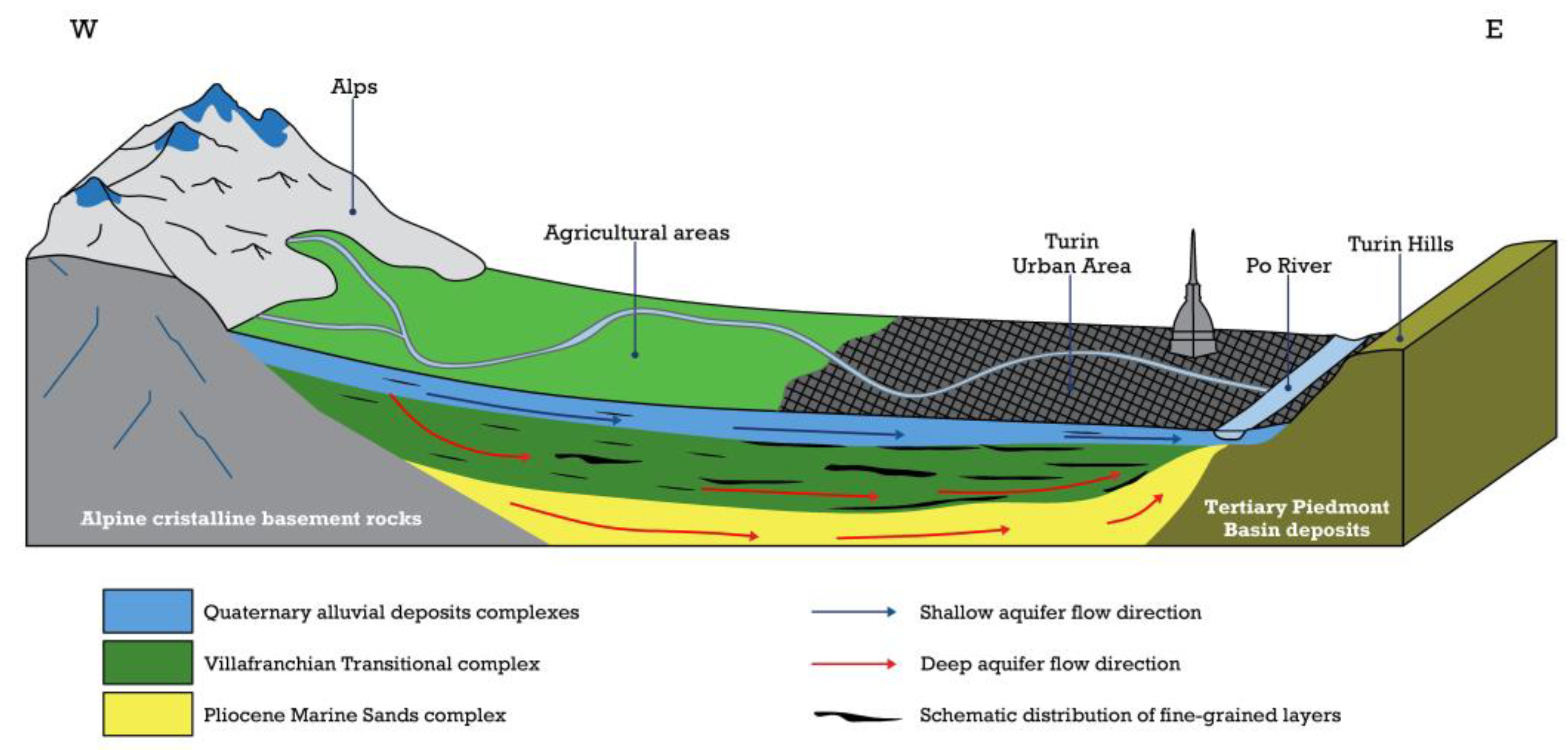
Figure 3.
Hydrogeological map and piezometric surface of the shallow aquifer in the Piedmont Po Plain (summer 2016) (modified from [63]).
Figure 3.
Hydrogeological map and piezometric surface of the shallow aquifer in the Piedmont Po Plain (summer 2016) (modified from [63]).
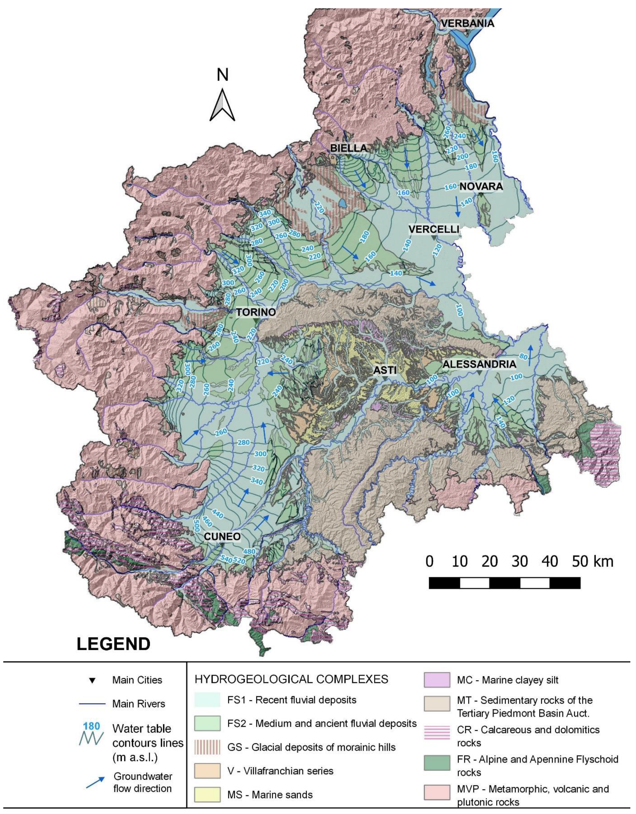
Figure 4.
Two hundred and twenty-seven selected monitoring wells in the Piedmont Po plain.

Figure 5.
Spatial representations of trend results for EC, HCO3, Ca and Mg.

Figure 6.
Spatial representation of trend results for pH.

Figure 7.
Spatial representations of trend results for NO3, SO4, Cl and Na.

Figure 8.
ChP occurrence based on seasons. (I): springs, (II): autumns, (NO): no ChP. Labels: number of monitoring wells.
Figure 8.
ChP occurrence based on seasons. (I): springs, (II): autumns, (NO): no ChP. Labels: number of monitoring wells.
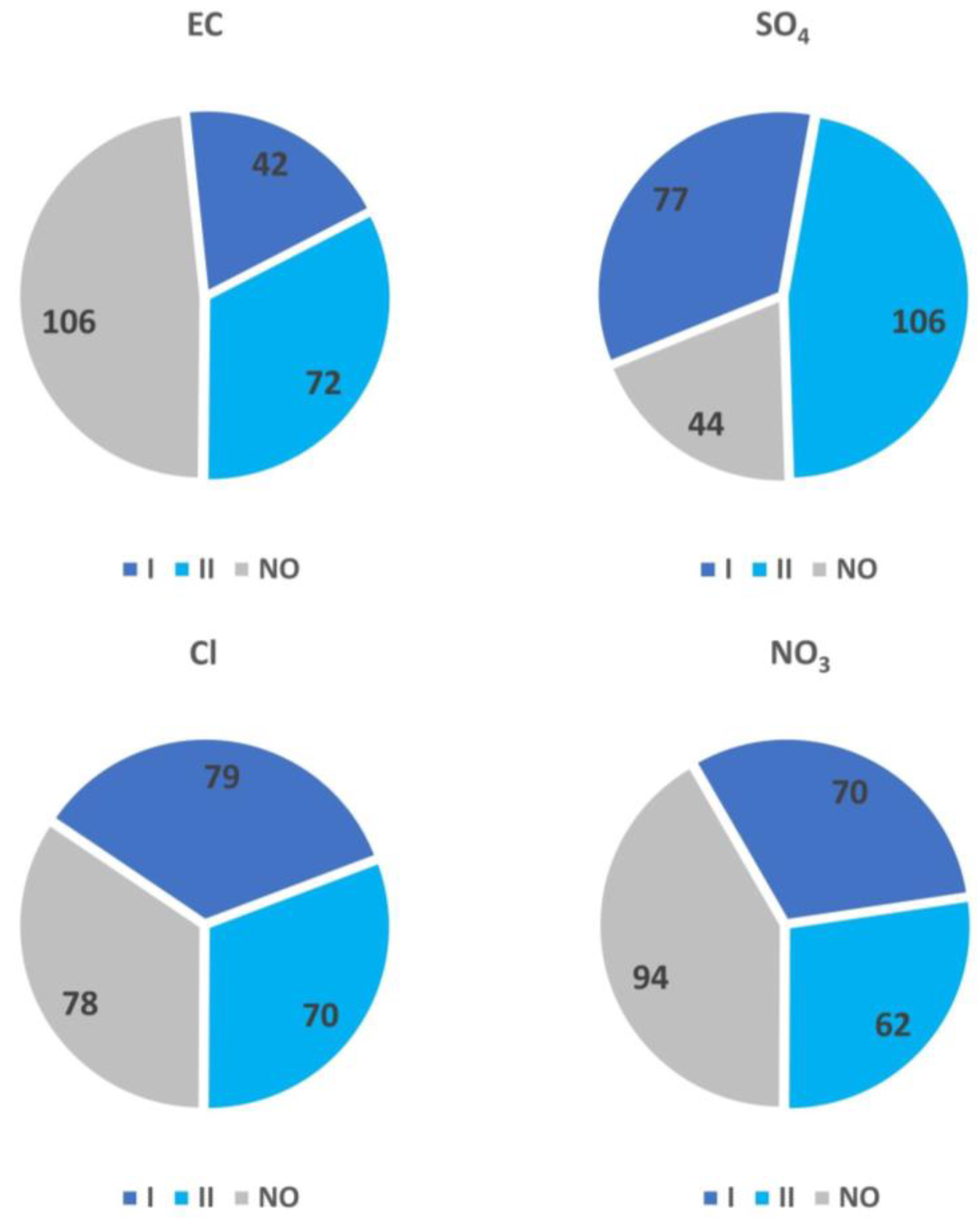
Figure 9.
ChP occurrence based on semestral sampling time moment. (I): springs, (II): autumns.
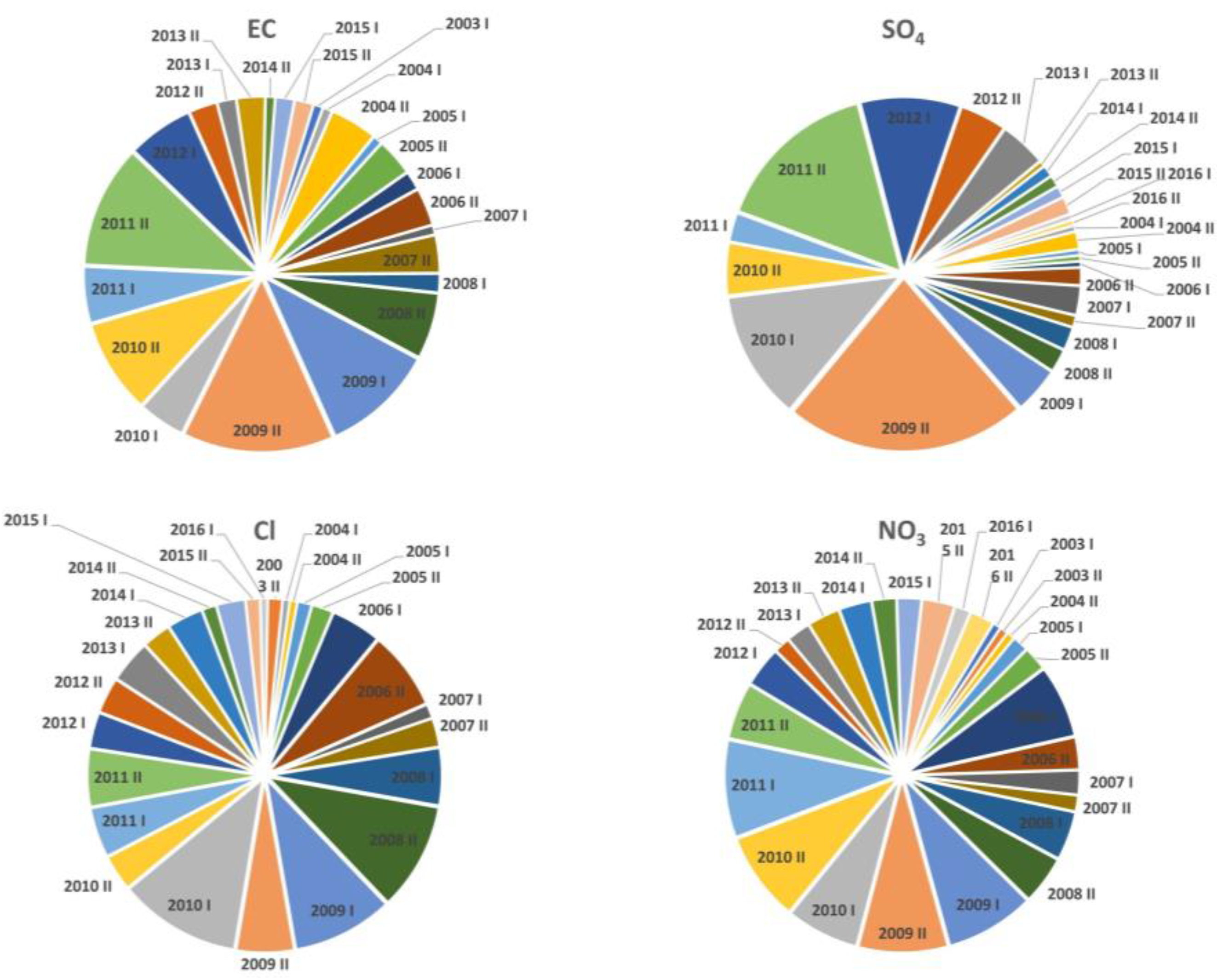
Figure 10.
Examples of direct proportionalities between groundwater chemistry and groundwater level without temporal lag.
Figure 10.
Examples of direct proportionalities between groundwater chemistry and groundwater level without temporal lag.
Figure 11.
Examples of monitoring wells with temporal lag. Red line: original time series of physicochemical parameter; green line: transposed time series of physicochemical parameter. The difference between them highlights the temporal lag.
Figure 11.
Examples of monitoring wells with temporal lag. Red line: original time series of physicochemical parameter; green line: transposed time series of physicochemical parameter. The difference between them highlights the temporal lag.
Figure 12.
(a,b) Examples of monitoring wells with seasonal fluctuation of groundwater level and heterogeneous physicochemical parameters variation; (c,d) examples of physicochemical parameter trends without groundwater level trends over time (groundwater level trend (dashed blue line), groundwater chemistry trend (dashed red line)).

Table 1.
Number of monitoring wells with increase (+), decrease (−) or no trends in the different physicochemical parameters. Prevailing behaviour underlined.
Table 1.
Number of monitoring wells with increase (+), decrease (−) or no trends in the different physicochemical parameters. Prevailing behaviour underlined.
| EC | HCO3 | Ca | Mg | Na | Cl | NO3 | SO4 | pH | |
|---|---|---|---|---|---|---|---|---|---|
| + | 70 | 78 | 64 | 58 | 122 | 93 | 40 | 16 | 21 |
| − | 53 | 16 | 38 | 55 | 25 | 38 | 88 | 156 | 35 |
| No Trend | 104 | 133 | 125 | 114 | 80 | 96 | 99 | 55 | 171 |
Table 2.
Quantification of OLS variations at regional level (expressed as mg/L (or μS/cm) and %).
| OLS | Trend | EC | HCO3 | Ca | Mg | NO3 | Cl | Na | SO4 | pH |
|---|---|---|---|---|---|---|---|---|---|---|
| Δ mg/L (μS/cm) | + | 172 | 43 | 17 | 4 | 12 | 31 | 19 | 25 | 0.4 |
| Δ mg/L (μS/cm) | − | 126 | 45 | 22 | 6 | 14 | 17 | 12 | 21 | 0.3 |
| Δ % | + | 20 | 21 | 26 | 22 | 55 | 54 | 48 | 58 | 5.0 |
| Δ % | − | 28 | 23 | 27 | 35 | 68 | 54 | 48 | 38 | 4.6 |
Disclaimer/Publisher’s Note: The statements, opinions and data contained in all publications are solely those of the individual author(s) and contributor(s) and not of MDPI and/or the editor(s). MDPI and/or the editor(s) disclaim responsibility for any injury to people or property resulting from any ideas, methods, instructions or products referred to in the content. |
© 2024 by the authors. Licensee MDPI, Basel, Switzerland. This article is an open access article distributed under the terms and conditions of the Creative Commons Attribution (CC BY) license (https://creativecommons.org/licenses/by/4.0/).
Share and Cite
MDPI and ACS Style
Cocca, D.; Lasagna, M.; De Luca, D.A. Groundwater Chemical Trends Analyses in the Piedmont Po Plain (NW Italy): Comparison with Groundwater Level Variations (2000–2020). Water 2024, 16, 1240. https://doi.org/10.3390/w16091240
AMA Style
Cocca D, Lasagna M, De Luca DA. Groundwater Chemical Trends Analyses in the Piedmont Po Plain (NW Italy): Comparison with Groundwater Level Variations (2000–2020). Water. 2024; 16(9):1240. https://doi.org/10.3390/w16091240
Chicago/Turabian StyleCocca, Daniele, Manuela Lasagna, and Domenico Antonio De Luca. 2024. "Groundwater Chemical Trends Analyses in the Piedmont Po Plain (NW Italy): Comparison with Groundwater Level Variations (2000–2020)" Water 16, no. 9: 1240. https://doi.org/10.3390/w16091240
Note that from the first issue of 2016, this journal uses article numbers instead of page numbers. See further details here.