Robust Adaptive Control of the Offshore Produced Water Treatment Process: An Improved Multivariable MRAC-Based Approach

Abstract

The application of deoiling hydrocyclone systems as the downstream of three-phase gravity separator (TPGS) systems is one of the most commonly deployed produced water treatment processes in offshore oil and gas production. Due to the compact system’s complexity and tailor-made features, it is always challenging to develop some optimally coordinated control solution for the coupled hydrocyclone and TPGS systems. It is obvious that coordinated control can better fulfill legislative discharge regulation by robustly maintaining high separation efficiencies. This paper presents a new control solution for a set of integrated hydrocyclone and TPGS systems by applying an improved multi-variable model reference adaptive control (MV-MRAC) approach with the aim of achieving both asymptotic output tracking and unknown disturbance rejection. A robust MV-MRAC controller design is proposed based on a control parameterization derived from a factorization of a high-frequency gain matrix $K_p=LDS$ as a product of three matrices, where L represents unity lower triangular, $D=sign\left(D\right)$ represents diagonal, and S represents positive definite, and a teaching–learning-based optimization (TLBO) algorithm for optimizing the adaption rates. The developed solution is analyzed and compared with a commonly deployed PI control solution on a model that is derived from a lab-scale produced water treatment process. This simulation study demonstrates the promising potential of the proposed control solution compared with the currently deployed PI control solution.

1. Introduction

1.1. Motivation

With the aim of achieving sustainable extraction and minimizing environmental pollution in offshore oil and gas production, the treatment of produced water (PW) is inevitable before reinjecting PW into the reservoir for enhanced oil recovery or discharging it into the ocean. To effectively remove hydrocarbon residuals in the PW stream through the PW treatment processes (i.e., deoiling processes), it has been evidenced that the coordinated controls of the upstream three-phase gravity separators (TPGSs) with the downstream deoiling hydrocyclones can play a vital role in maintaining high deoiling efficiencies subjected to diverse disturbances [1].

Plant-wide control can be one of the promising strategies in handling this kind of challenge [2]. For example, by modeling the hydrocyclone and TPGSs in a coupled formulation, a number of advanced control solutions have been proposed for a class of deoiling processes, such as $H_{\infty }$ control [1], nonlinear MPC [3], feedback linearization control [4], etc. Moreover, comparisons of different control solutions can be observed in [5].

Different from the aforementioned control solutions, in this work, we explore a plant-wide MRAC solution for handling the coordinated control of the coupled hydrocyclone and TPGS systems, with respect to the MRAC’s unique feature, that is, this type of controller can automatically adapt to certain uncertainties without scarifying the system’s performance, including variations in dynamic characteristics, via its simple online learning capability; therefore, it can be less conservative in demands of control and modeling efforts [6].

1.2. State of the Art

From the plant-wide control perspective, by focusing on the upstream riser of the TPGS system, Pedersen et al. [7] investigated antislugging control by automatically choking the feeding control valve of the separator to mitigate the significant dynamic variation induced by slugging flow into the separator system. Moreover, several control approaches were evaluated in order to address the challenges posed by slugging flow in offshore oil production [8]. The control designs consist of feedback linearization, gain scheduling, internal model control (IMC), PI control with an adaptive gain, and state feedback with state estimation by an observer. To determine their effectiveness, these controllers were examined in terms of their robustness to inflow disturbances and time delays. Durdevic et al. [1] developed an $H_{\infty }$ robust control for the coupled hydrocyclone and TPGS systems and compared it to a benchmark PID control solution. Li et al. investigated the design of $H_{\infty }$ control using model-free off-policy reinforcement learning in [9].

By focusing on the OiW concentration limitation (e.g., <30 ppm dispersed hydrocarbon compounds) in the effluent water out of the deoiling hydrocyclone, Vallabhan et al. investigated a control solution based on their pilot plant in [10]. Moreover, a nonlinear MPC control strategy was developed to predict the dynamic behavior of the pressure near the bottom of the production column [11]. Most control solutions mentioned have fixed structures, except MPC, which offers flexibility but demands a robust implementation platform for online optimization. Therefore, adaptive control strikes a balance between flexibility and simplicity by continuously tuning control parameters based on real-time feedback. In addition, adaptive control solutions offer a dynamic approach to handling uncertainties and variations in real time, ensuring optimal performance in changing conditions [6]. Based on the authors’ research, there appears to be a lack of adaptive control solutions implemented or undergoing testing for offshore PW treatment processes from a global perspective. Consequently, in response to this gap, we have developed an MRAC state feedback system for achieving output tracking in offshore PW treatment, accounting for uncertainties in system parameters and input–output disturbances [12].

As one of the popularly used adaptive control methods, the MRAC can be classified into different schemes characterized by using either output or state feedback for tracking performance. In general, there are (a) MRACs using state feedback for state tracking; (b) MRACs using state feedback for output tracking; and (c) MRACs using output feedback for output tracking [13]. An extended MRAC scheme was proposed in [14] using the partial state feedback based on the LDS decomposition of the plant high-frequency gain matrix to ensure asymptotic output tracking and system stability. The same approach was adopted in [15,16] to design flight controls subject to diverse turbulence conditions. A robust output feedback MRAC with output tracking was investigated in [17] based on the reinforced dead-zone modification in the presence of actuator faults, modeling uncertainty, and output disturbance. Hua et al. [18] proposed a decentralized state feedback MRAC approach for large-scale reactor systems with time-varying delays.

1.3. Contributions

The MRAC method has made significant progress in recent decades, but challenges remain. One key challenge is its robustness for uncertain multivariable systems with unknown disturbances. This paper addresses this challenge by developing a robust multi-input multi-output (MIMO) MRAC solution. The solution is applied to a deoiling process comprising a TPGS system coupled with downstream hydrocyclone systems, mimicking offshore produced water treatment processes. The developed solution utilizes output feedback to handle output tracking and unknown disturbance rejection, considering model uncertainties. To enhance system performance, an augmented error is employed in the adaptation law of the controller, and the TLBO algorithm is utilized to achieve optimal adaptation rates. Additionally, an LDS decomposition of the high-frequency gain matrix is incorporated into the adaptive controller to eliminate the need for a priori knowledge of this matrix. Stability and asymptotic tracking performance of the closed-loop system are guaranteed by Lyapunov stability and Barbalat’s Lemma. In summary, the contributions of this article can be listed as follows:

• A novel control solution is presented for integrated hydrocyclone and TPGS systems, utilizing a robust MV-MRAC with respect to unknown disturbance.
• LDS decomposition is implemented in the proposed method to eliminate the constraint of a priori knowledge of the high-frequency gain matrix.
• To reach stable adaptive laws, the controller’s adaptive laws are formulated by considering augmented error, which encompasses parameters and tracking errors.
• A new multi-objective optimization problem is presented for optimizing the controller’s adaptation rates, which is solved using the TLBO algorithm.

The rest of the paper is organized as follows: Section 2 introduces the considered system and process; Section 3 formulates the robust MV-MRAC problem; Section 4 presents the design procedure; Section 5 illustrates diverse simulation results; and finally, we conclude the paper in Section 6.

2. Deoiling Process Model

In this section, a comprehensive exploration of the deoiling process model is presented. This exploration is divided into two subsections. In the following, the considered separation system as well as the model development are presented.

Considered Separation System

Produced water is an inevitable by-product during oil and gas production, and the water cut gradually increases as reservoirs mature. Whether the produced water is re-injected into reservoirs for enhanced oil recovery, or simply discharged to the oceans, the hydrocarbon compounds (sometimes also referred to as oil residuals) in the produced water must be limited to avoid formation damage and to comply with the regional discharge limits. Therefore, the produced water needs to be properly treated before re-injection or discharge.

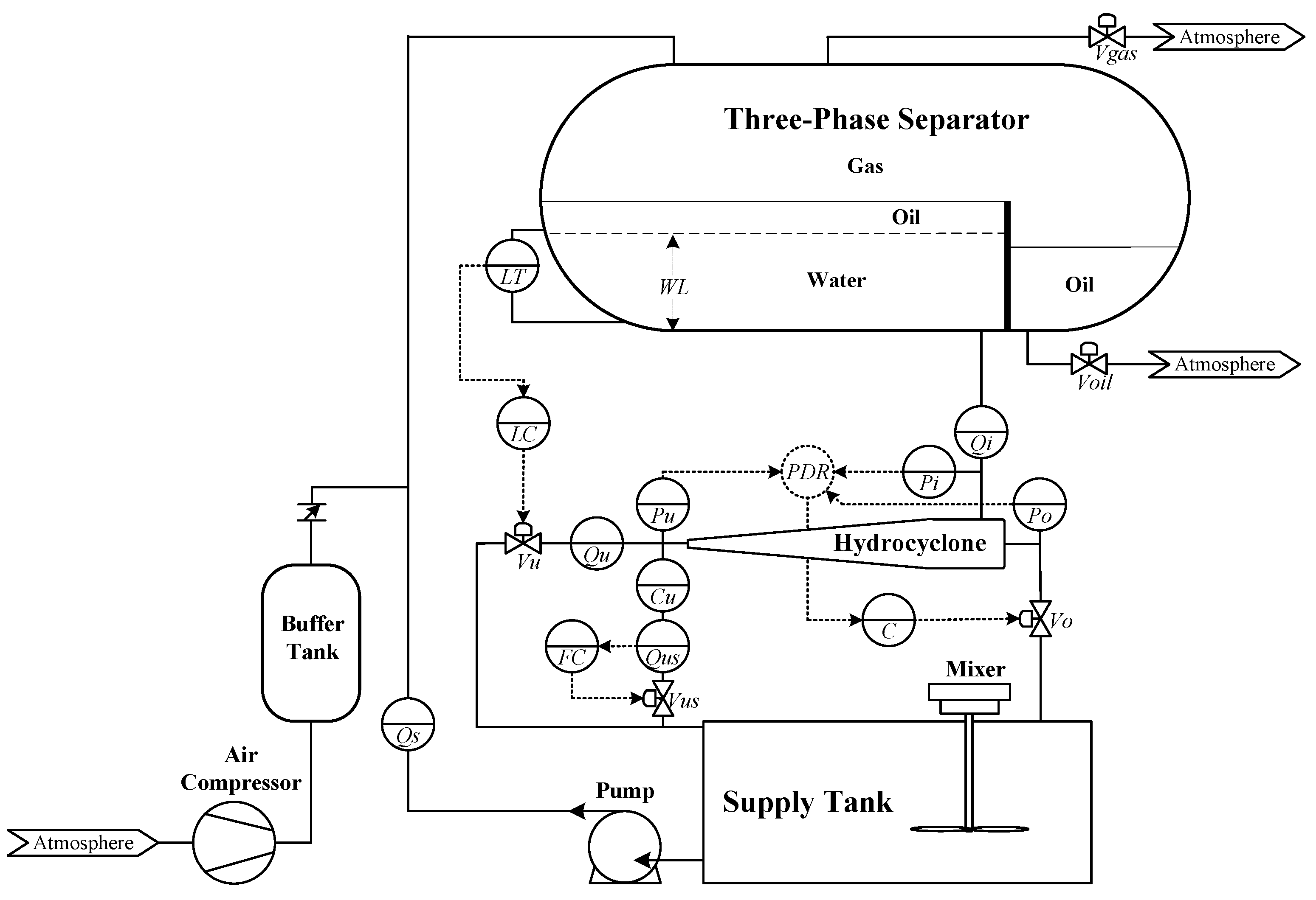
Figure 1 shows the experimental setup used in this study, which mimics an offshore produced water treatment facility. The system consists of a mixing tank with a centrifugal pump and an air compressor which acts as the reservoir. A vertical pipeline riser directs the multiphase flow into the TPGS tank, where the gas, oil, and water are separated based on their density differences. The gas rises to the top of the separator where it exits through the gas control valve ($V_{gas}$), which is operated by the separator pressure controller. The oil is separated from the water as it skims over a weir plate and enters the oil compartment. The interphase level between the oil and water is measured by a level transmitter (denoted LT) and controlled by the level controller (denoted LC) by actuating the underflow valve (denoted $V_u$). This control loop keeps the water below the top of the weir plate and above the water outlet to maintain product quality and separator pressure. The water from the three-phase separator is cleaned further using hydrocyclones which separate oil and water based on enhanced gravity separation. Due to the tangential inlet and the hydrocyclone geometry, a vortex is generated inside. The centripetal force generated pushes the oil droplets toward the hydrocyclone centerline, where an oil core is formed. The cleaned water leaves through the hydrocyclone underflow, while the oil is discharged through the hydrocyclone overflow. Usually, the hydrocyclone system is operated by controlling the overflow control valve ($V_o$) via a pressure drop ratio (PDR) control loop. The two separation systems are coupled via these control mechanisms [1]. Moreover, the development of the system model is detailed in Appendix A below.

3. Prerequisites for Robust MV-MRAC Design

The prerequisites for designing a robust MRAC with output tracking subject to unknown disturbances and unmatched system uncertainties are given below.

3.1. System Model

Consider a MIMO LTI system subject to disturbance $d_j\left(t\right)$, presented in state space formulation as [19]:

$$\begin{array}{c}\dot{x}\left(t\right)=Ax\left(t\right)+Bu\left(t\right)+B_d{d}_j\left(t\right)\\ y\left(t\right)=Cx\left(t\right),\end{array}$$

(1)

It is assumed that the system is controllable and observable. The system matrices denoted as $A\in {\mathbb{R}}^{n\times n}$, $B\in {\mathbb{R}}^{n\times M}$, $B_d\in {\mathbb{R}}^{n\times q}$, and $C\in {\mathbb{R}}^{M\times n}$ are unknown (for the designer). $x\left(t\right)\in {\mathbb{R}}^n$, $y\left(t\right)\in {\mathbb{R}}^M$, $u\left(t\right)\in {\mathbb{R}}^M$ are the system’s state, output, and the control input vectors, respectively. The actuation disturbance $d_j\left(t\right)\in {\mathbb{R}}^q$ has components characterized by Equation (2), where $d_{j0}$, $d_{jk}$ are unknown constants and ${\Omega }_{jk}\left(t\right)$ for $j=1,\cdots ,q,k=1,\cdots ,p_j$ are the known bounded continuous-time signals [20].

$$d_j\left(t\right)=d_{j0}+\sum _{k=1}^{p_j}{d}_{jk}{\Omega }_{jk}\left(t\right),j=1,2,\dots ,q.$$

(2)

As stated in [6], this disturbance model, which encompasses sinusoidal, non-sinusoidal, and constant-valued disturbances, can efficiently approximate a broad range of disturbances found in different control applications. For example, if $p_j$ is selected as one and ${\Omega }_{j1}\left(t\right)=sin\left({\omega }_{j1}t\right)$, then this specific $d_j\left(t\right)=d_{j0}+d_{j1}sin\left({\omega }_{j1}t\right)$ represents a periodic disturbance. If $p_j$ is set to zero, then $d_j\left(t\right)=d_{j0}$, $j=1,2,\dots ,q$ representing some constant disturbance signals [21]. The input–output description form of the system, presented by Equation (1), is given as:

$$y\left(t\right)=G\left(s\right)u\left(t\right)+\overline{y}\left(t\right),$$

(3)

in which $G\left(s\right)\widehat{=}C{(sI-A)}^{-1}B$ and $\overline{y}\left(t\right)\widehat{=}C{(sI-A)}^{-1}{B}_d{d}_j\left(t\right)$.

3.2. Modified Left Interactor and Reference Model

The modified left interactor (MLI) is an important concept in designing multivariable adaptive control.

Theorem [6]: There exists a unique lower triangular polynomial matrix ${\xi }_m\left(s\right)$, as shown in Equation (4), for any $M\times M$ strictly proper and full rank matrix $G\left(s\right)$, and this matrix is defined as the modified left interactor (MLI) matrix of $G\left(s\right)$ [22].

$${\xi }_m\left(s\right)\widehat{=}\left[\begin{array}{ccccc}{g}_1\left(s\right)& 0& \cdots & \cdots & 0\\ h_{21}^m\left(s\right)& g_2\left(s\right)& 0& \cdots & 0\\ ⋮& ⋮& ⋮& ⋮& ⋮\\ h_{M1}^m\left(s\right)& \cdots & \cdots & h_{MM-1}^m\left(s\right)& g_M\left(s\right)\end{array}\right],$$

(4)

where $h_{ij}^m\left(s\right)$, j = 1, …, M − 1, i = 2, …, M, are polynomials, and $g_i\left(s\right)$, i = 1, …, M are monic stable polynomials of degrees $l_i>0$.

The MLI matrix has the following relationship with the high-frequency gain (HFG) matrix of $G\left(s\right)$ as

$$\underset{s\to \infty }{lim}{\xi }_m\left(s\right)G\left(s\right)=K_p,$$

(5)

where matrix $K_p\in {\mathbb{R}}^{M\times M}$ is finite and non-singular.

Assume that the reference output $y_m\left(t\right)$ is generated by a reference model with given reference signal $r\left(t\right)$ from

$$y_m\left(t\right)=W_m\left(s\right)r\left(t\right), \mathrm{where} W_m\left(s\right)={\xi }_m^{-1}\left(s\right).$$

(6)

Reference $r\left(t\right)\in {\mathbb{R}}^M$ is assumed bounded and piece-wise continuous. $W_m\left(s\right)\in {\mathbb{R}}^{M\times M}$ is a stable transfer function matrix chosen from the inverse of the MLI matrix ${\xi }_m$ defined by Equation (4).

3.3. System Assumptions

The design assumptions are summarized as:

• (A.1) $G\left(s\right)$ is strictly proper and full rank, and its MLI matrix ${\xi }_m\left(s\right)$ is also known, such that the reference model is selected as $W_m\left(s\right)={\xi }_m^{-1}\left(s\right)$.
• (A.2) All transmission zeros of $G\left(s\right)$ lie on the left of the imaginary axis, and the $(A,B,C)$ system is stabilizable and detectable.
• (A.3) All leading principal minors ${\Delta }_i$ of the HFG matrix $K_p$ are nonzero with known signs.
• (A.4) An upper bound $\overline{\nu }$ is known on observability index of $G\left(s\right)$. Transfer function models of the system from the control input and disturbance input are presented in their left coprime polynomial matrix decomposition, i.e., $G\left(s\right)=P_l^{-1}\left(s\right)Z_0\left(s\right)$ and $G_d\left(s\right)=P_l^{-1}\left(s\right)Z_d\left(s\right)$, where $P_l\left(s\right)$, $Z_0\left(s\right)\in {\mathbb{R}}^{M\times M}$ and $Z_d\left(s\right)\in {\mathbb{R}}^{M\times q}$ are proper polynomial matrices.
• (A.5) The relative degree condition is established such that $Z_0^{-1}\left(s\right)Z_d\left(s\right)$ is proper.

Assumption A.1 is considered to select a stable reference model system $W_m\left(s\right)$ for plant model matching. Condition A.2 guarantees that none of the zeros lead $G\left(s\right)$ to lose its rank, which might risk the system becoming uncontrollable. A.3 is applied to guarantee the adaptive parameter update laws are stable and converge. Condition A.4 is needed to filter the input and output signals for constructing an adaptive output feedback controller structure suitable for plant model matching. A.5 specifies a condition for the MRAC scheme for disturbance rejection [15].

3.4. Output Feedback Control Structure

The control signal generated by a standard output feedback output tracking MRAC has the following compositions:

$$u\left(t\right)={\Theta }_1^T\left(t\right){\omega }_1\left(t\right)+{\Theta }_2^T\left(t\right){\omega }_2\left(t\right)+{\Theta }_{20}\left(t\right)y\left(t\right)+{\Theta }_3\left(t\right)r\left(t\right)+{\Theta }_4\left(t\right),$$

(7)

where ${\Theta }_1={[{\Theta }_{11},\cdots ,{\Theta }_{1j},\cdots ,{\Theta }_{1\overline{\nu }-1}]}^T$, and ${\Theta }_2={[{\Theta }_{21},\cdots ,{\Theta }_{2j},\cdots ,{\Theta }_{2\overline{\nu }-1}]}^T$ are the adaptation gain matrices for the filtered input and output signals, respectively. Here ${\Theta }_{ij}\in R^{M\times M}$, where $i=1,2,j=1,\cdots ,\overline{\nu }-1$, with $\overline{\nu }$ representing the observability index (or its upper bound $\overline{\nu }$) of the plant $G\left(s\right)$. Respectively, the filtered input and output signals are ${\omega }_1\left(t\right)=F\left(s\right)u\left(t\right)$, ${\omega }_2\left(t\right)=F\left(s\right)y\left(t\right)$, where filter $F\left(s\right)=\frac{A\left(s\right)}{\Lambda \left(s\right)}$ with $A\left(s\right)={[I_M,s{I}_M,\cdots ,s^{\overline{\nu }-2}{I}_M]}^T$, and a monic stable polynomial $\Lambda \left(s\right)$ of degree $\overline{\nu }-1$. Moreover, ${\Theta }_{20}\in R^{M\times M}$ is adaptation gain matrix for output signal $y\left(t\right)$ and ${\Theta }_3\in R^{M\times M}$ is adaptation gain matrix for reference signal $r\left(t\right)$, and ${\Theta }_4\in R^{M\times M}$ is employed to reject the effects induced by the disturbance $d_j\left(t\right)$ [23].

3.5. Plant Model Matching Condition

If the system and disturbance parameters are all known and constant, the steady-state (optimal) output feedback control can be presented by:

$$u^{*}\left(t\right)={\Theta }_1^{*T}{\omega }_1\left(t\right)+{\Theta }_2^{*T}{\omega }_2\left(t\right)+{\Theta }_{20}^{*}y\left(t\right)+{\Theta }_3^{*}r\left(t\right)+{\Theta }_4^{*}\left(t\right),$$

(8)

where these steady-state values of parameters ${\Theta }_1^{*T},{\Theta }_2^{*T},{\Theta }_{20}^{*},{\Theta }_3^{*},{\Theta }_4^{*}$ are not a priori, but their existence needs to be assumed.

The plant model matching condition is satisfied by Equation (9) when parameters ${\Theta }_1^{*T},{\Theta }_2^{*T}$, ${\Theta }_{20}^{*},{\Theta }_3^{*}$ meet the final value theorem condition under the assumption that $d_j\left(t\right)=0$, i.e.,

$$I-{\Theta }_1^{*T}F\left(s\right)-{\Theta }_2^{*T}F\left(s\right)G\left(s\right)-{\Theta }_{20}^{*}G\left(s\right)={\Theta }_3^{*}{W}_m^{-1}\left(s\right)G\left(s\right).$$

(9)

To realize the desired disturbance rejection, by substituting Equation (3) into Equation (8), the closed-loop system is given as:

$$\begin{array}{cc}\hfill y\left(t\right)& =G\left(s\right){\left[{\Theta }_3^{*}{W}_m^{-1}\left(s\right)G\left(s\right)\right]}^{-1}[{\Theta }_2^{*T}F\left(s\right)\left[\overline{y}\right]\left(t\right)+{\Theta }_{20}^{*}\overline{y}+{\Theta }_3^{*}r+{\Theta }_4^{*}]+\overline{y}\left(t\right)\hfill \\ \hfill & =W_m\left(s\right)r\left(t\right)+W_m\left(s\right)+K_p[\frac{(-{\Theta }_1^{*T}A\left(s\right)P\left(s\right)+\Lambda \left(s\right)P\left(s\right))Z_a^{-1}\left(s\right)}{\Lambda \left(s\right)}\overline{y}+{\Theta }_4^{*}]\left(t\right)\hfill \\ \hfill & =W_m\left(s\right)r\left(t\right)+V_p\left(t\right),\hfill \end{array}$$

(10)

where ${\Theta }_3^{*}=K_p^{-1}$ and the term $V_p\left(t\right)$ is

$$\begin{array}{c}\hfill V_p\left(t\right)=W_m\left(s\right){\Theta }_3^{*-1}[{\Theta }_2^{*T}F\left(s\right)\overline{y}\left(t\right)+{\Theta }_{20}^{*}\overline{y}+{\Theta }_3^{*}{W}_m^{-1}\left(s\right)\overline{y}\left(t\right)+{\Theta }_4^{*}]\left(t\right).\end{array}$$

(11)

One potential selection is to consider $V_p\left(t\right)=0$ to eliminate the impact of the disturbance. Consequently,${\Theta }_4^{*}\left(t\right)$ is determined as follows:

$${\Theta }_4^{*}\left(t\right)=-{\Theta }_3^{*}{W}_m^{-1}\left(s\right)\overline{y}\left(t\right)-{\Theta }_{20}^{*}\overline{y}\left(t\right)-{\Theta }_2^{*T}F\left(s\right)\overline{y}\left(t\right).$$

(12)

Thereby, Equation (11) can be rewritten as follows:

$$V_p\left(t\right)=W_m\left(s\right)K_p[\frac{P_{\alpha }\left(s\right)Z_d\left(s\right)}{\Lambda \left(s\right)}{d}_j\left(t\right)+{\Theta }_4^{*}]\left(t\right),$$

(13)

According to [6], there is a polynomial matrix $P_{\alpha }\left(s\right)$ such that it satisfies

$$\begin{array}{c}\hfill \Lambda \left(s\right)I\left(s\right)-{\Theta }_1^{*T}A\left(s\right)=P_{\alpha }\left(s\right)Z_0\left(s\right),\\ \hfill {\displaystyle \underset{s\to \infty }{lim}\frac{P_{\alpha }\left(s\right)}{\Lambda \left(s\right)}{Z}_d\left(s\right)<\infty .}\end{array}$$

(14)

Then ${\Theta }_4^{*}$ can be chosen as:

$${\Theta }_4^{*}\left(t\right)=-\frac{P_{\alpha }\left(s\right)Z_d\left(s\right)}{\Lambda \left(s\right)}{d}_j\left(t\right).$$

(15)

Thereby, the complete disturbance rejection at the system output can be achieved if ${\displaystyle \frac{P_{\alpha }\left(s\right)}{\Lambda \left(s\right)}{Z}_d\left(s\right)}$ is proper [24].

3.6. Linear Parametrization of ${\Theta }_4^{*}\left(t\right)$

A linear parametrization of ${\Theta }_4^{*}\left(t\right)$ is essential for effective adaptive controller design with guaranteed asymptotic tracking property. According to assumption A.5, ${\Theta }_4^{*}\left(t\right)$ can be rewritten as follows:

$${\Theta }_4^{*}\left(t\right)={\Theta }_q^{*}\frac{A_q\left(s\right)}{\Lambda \left(s\right)}{d}_j\left(t\right)+{\Theta }_0^{*}{d}_j\left(t\right),$$

(16)

where ${\Theta }_q^{*}=[{\Theta }_{q1}^{*},{\Theta }_{q2}^{*},\cdots ,{\Theta }_{q(\overline{\nu }-1)}^{*}]\in {\mathbb{R}}^{M\times q(\overline{\nu }-1)}$ with ${\Theta }_{qj}^{*}\in {\mathbb{R}}^{M\times q}$ and ${\Theta }_0\in {\mathbb{R}}^{M\times q}$ are constant parameter matrices. Additionally, define $A_q\left(s\right)={[I_q,s{I}_q,\cdots ,s^{\overline{\nu }-2}{I}_q]}^T$ with $I_q\in {\mathbb{R}}^{q\times q}$. As mentioned earlier, the disturbance expression, as defined in Equation (2), can be expressed as follows:

$$d_j\left(t\right)={\varphi }_j^{*T}{\psi }_j\left(t\right)$$

(17)

where

$$\begin{array}{cc}\hfill {\varphi }_j^{*}& ={[{\overline{d}}_{j0},{\overline{d}}_{j1},\cdots ,{\overline{d}}_{jpj}]}^T\hfill \\ \hfill {\psi }_j\left(t\right)& ={[1,{\Omega }_{j1}\left(t\right),\cdots ,{\Omega }_{jpj}\left(t\right)]}^T\in {\mathbb{R}}^{pj+1}\hfill \end{array}$$

(18)

$d_j\left(t\right)\in {\mathbb{R}}^q$ can also be expressed as:

$$d_j\left(t\right)={\Phi }^{*T}\Psi \left(t\right),$$

(19)

where

$$\begin{array}{cc}\hfill {\Phi }^{*T}& =\left[\begin{array}{ccccc}{\varphi }_1^{*}& {\varphi }_{(p1+1)}^{*}& {\varphi }_{(p1+1)}^{*}& \cdots & 0_{(p1+1)}\\ 0_{(p2+1)}& {\varphi }_2^{*}& 0_{(p2+1)}& \cdots & 0_{(p2+1)}\\ 0_{(p3+1)}& 0_{(p3+1)}& {\varphi }_3^{*}& \cdots & 0_{(p3+1)}\\ ⋮& ⋮& ⋮& \ddots & ⋮\\ 0_{(p_q+1)}& 0_{(p_q+1)}& 0_{(p_q+1)}& \cdots & {\varphi }_q^{*}\end{array}\right],\hfill \\ \hfill \Psi \left(t\right)& =\begin{array}{c}{[{\psi }_1^T\left(t\right),{\psi }_2^T\left(t\right),\cdots ,{\psi }_q^T\left(t\right)]}^T\in {\mathbb{R}}^{n_{\psi }}\end{array},\hfill \\ \hfill n_{\psi }& =\sum _{j=1}^q{p}_j+q,\hfill \end{array}$$

(20)

with $0_{(pj+1)}\in R^{pj+1}$ being a zero vector. Based on Equation (19), parameterization of ${\Theta }_4^{*}$ can be modified as follows:

$${\Theta }_4^{*}\left(t\right)={\Theta }_5^{*T}{\omega }_5\left(t\right)$$

(21)

where the parameterized variables are presented as follows:

$${\Theta }_5^{*}={[{\Theta }_{q1}^{*}{\Phi }^{*T},\cdots ,{\Theta }_{q({\overline{\nu }}_0-1)}^{*}{\Phi }^{*T}]}^T,$$

(22)

$${\omega }_5\left(t\right)={[{(\frac{A_q\left(s\right)}{\Lambda \left(s\right)}\Psi \left(t\right))}^T,{\Psi }^T\left(t\right)]}^T,$$

(23)

$$A_q\left(s\right)={[I_{n_{\psi }},s{I}_{n_{\psi }},\cdots ,s^{{\overline{\nu }}_0-2}{I}_{n_{\psi }}]}^T.$$

(24)

Hence, the nominal controller structure can be rewritten as:

$$u^{*}\left(t\right)={\Theta }_1^{*T}{\omega }_1\left(t\right)+{\Theta }_2^{*T}{\omega }_2\left(t\right)+{\Theta }_{20}^{*}y\left(t\right)+{\Theta }_3^{*}r\left(t\right)+{\Theta }_5^{*}\left(t\right){\omega }_5$$

(25)

3.7. LDS Decomposition

Definition: Any $M\times M$ real matrix $K_p$ with nonzero leading principal minors can be factored as follows:

$$K_p=LDS$$

(26)

where L is an $M\times M$ unit lower triangular matrix, $S\in {\mathbb{R}}^{M\times M}$ is a symmetric positive definite matrix, and

$$D=diag\left\{sign\left[{\Delta }_1\right]{\gamma }_1,\cdots ,sign\left[\frac{{\Delta }_M}{{\Delta }_{M-1}}\right]{\gamma }_M\right\}$$

(27)

is also non-unique, in which ${\Delta }_i$ is the leading principle minors of $K_p$ and ${\gamma }_i>0,i=1,\cdots ,M$, is an arbitrary positive diagonal matrix [6]. To cope with the restrictive design conditions and the uncertainty in $K_p$ caused by the plant uncertainties, the LDS decomposition is applied to design a robust output feedback MRAC.

4. Robust MRAC Design

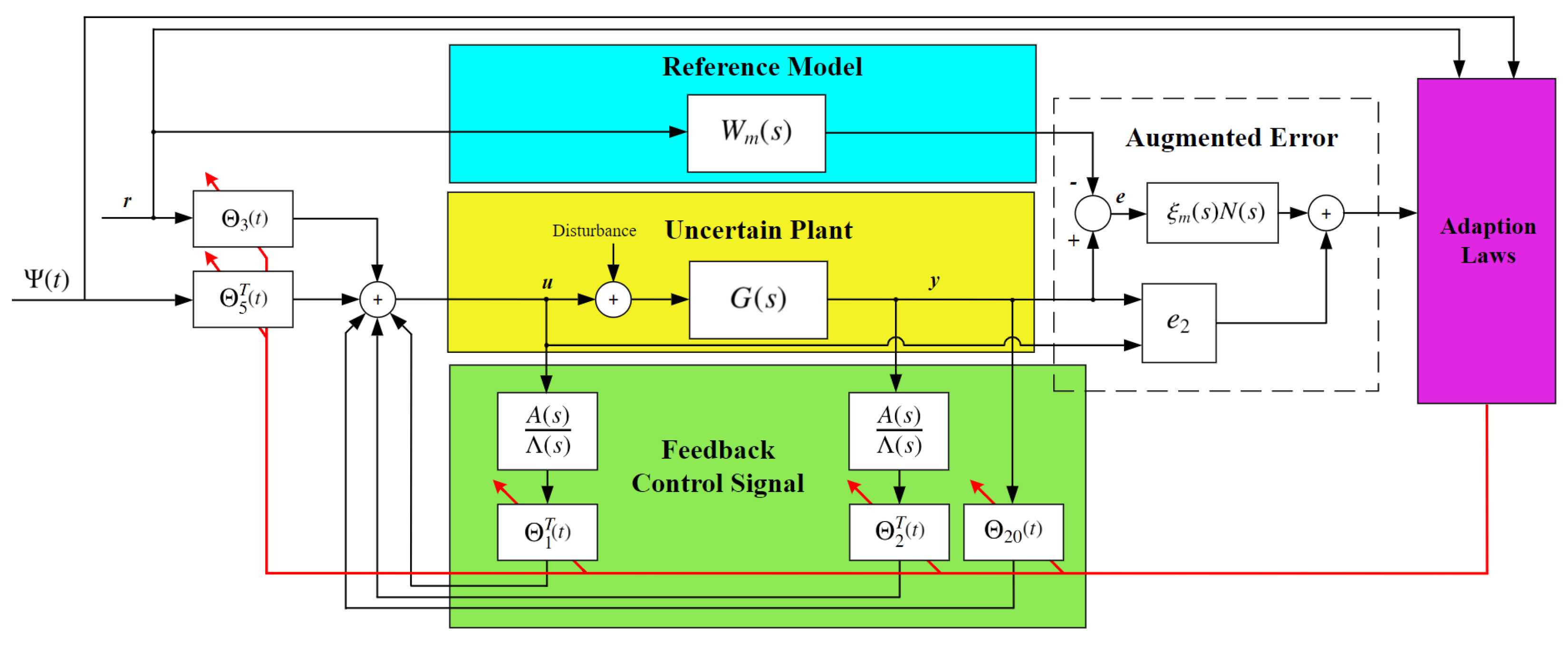
In the presence of system parameter uncertainties and unknown disturbances, the nominal controller is no longer sufficient. Therefore, an adaptive version of this controller needs to be designed. The adaptive architecture corresponding to Equation (25) is stated as:

$$u\left(t\right)={\Theta }_1^T\left(t\right){\omega }_1\left(t\right)+{\Theta }_2^T\left(t\right){\omega }_2\left(t\right)+{\Theta }_{20}\left(t\right)y\left(t\right)+{\Theta }_3\left(t\right)r\left(t\right)+{\Theta }_5^T\left(t\right){\omega }_5\left(t\right),$$

(28)

where ${\Theta }_1^T\left(t\right)$, ${\Theta }_2^T\left(t\right)$, ${\Theta }_{20}\left(t\right)$, ${\Theta }_3\left(t\right)$, and ${\Theta }_5\left(t\right)$ are adjusted by the parameter update law through adaptive control. The proposed robust MRAC structure and parameterization are illustrated in Figure 2.

4.1. Adaptive Law Design

To design an adaptive controller as shown in Equation (28), the error equation in terms of tracking errors and parameter errors is a fundamental concept upon which adaptive laws are developed. Therefore, to achieve the error equation, both sides of Equation (9) are operated by $u\left(t\right)$ as:

$$u\left(t\right)-{\Theta }_1^{*T}F\left(s\right)u\left(t\right)-{\Theta }_2^{*T}F\left(s\right)G\left(s\right)u\left(t\right)-{\Theta }_{20}^{*}G\left(s\right)u\left(t\right)={\Theta }_3^{*}{W}_m^{-1}\left(s\right)G\left(s\right)u\left(t\right).$$

(29)

Replacing the system description (3) into Equation (29) we have

$$u\left(t\right)-{\Theta }_1^{*T}F\left(s\right)u\left(t\right)-{\Theta }_2^{*T}F\left(s\right)[y-\overline{y}]\left(t\right)-{\Theta }_{20}^{*}(y\left(t\right)-\overline{y}\left(t\right))={\Theta }_3^{*}{W}_m^{-1}\left(s\right)[y-\overline{y}]\left(t\right).$$

(30)

Replacing (6) in the above Equation (30), leads to

$$u\left(t\right)-{\Theta }_1^{*T}{\omega }_1\left(t\right)+{\Theta }_2^{*T}{\omega }_2\left(t\right)-{\Theta }_{20}^{*}y\left(t\right)+{\Theta }_3^{*}r\left(t\right)-{\Theta }_4^{*}={\Theta }_3^{*}{W}_m^{-1}\left(s\right)[y-\overline{y}\left(t\right)]\left(t\right),$$

(31)

where ${\Theta }_3^{*}=K_p^{-1}$ and ${\Theta }_4^{*}=-{\Theta }_3^{*}{W}_m^{-1}\left(s\right)\overline{y}\left(t\right)-{\Theta }_{20}^{*}\overline{y}\left(t\right)-{\Theta }_2^{*T}F\left(s\right)\left[\overline{y}\right]\left(t\right)$, which is obtained from (12). Then, (31) is obtained below:

$$K_p(u\left(t\right)-{\Theta }_1^{*T}{\omega }_1\left(t\right)-{\Theta }_2^{*T}{\omega }_2\left(t\right)-{\Theta }_{20}^{*}y\left(t\right)-{\Theta }_3^{*}r\left(t\right)-{\Theta }_4^{*}\left(t\right))=W_m^{-1}\left(s\right)\left[e\right]\left(t\right).$$

(32)

Substituting the gain matrix decomposition $K_p=LDS$ into Equation (32) leads to

$$\begin{array}{c}DS(u\left(t\right)-{\Theta }_1^{*T}{\omega }_1\left(t\right)-{\Theta }_2^{*T}{\omega }_2\left(t\right)-{\Theta }_{20}^{*}y\left(t\right)-{\Theta }_3^{*}r\left(t\right)-{\Theta }_4^{*}\left(t\right))\\ =L^{-1}{\xi }_m\left(s\right)[y-y_m]\left(t\right).\end{array}$$

(33)

If the controller described as (28) is performed with ${\Theta }_i={\Theta }_i^{*}$, it results in term ${\xi }_m\left(s\right)[y-y_m]\left(t\right)=0$, that is, ${\displaystyle \underset{t\to \infty }{lim}(y\left(t\right)-y_m\left(t\right))=0}$ exponentially.

4.2. Error Model

To obtain adaptive parameter update laws, an error model should be considered and driven based on the tracking error $e\left(t\right)=y\left(t\right)-y_m\left(t\right)$ and the parameter estimation error $\tilde{\Theta }\left(t\right)$. Hence, by substituting (28) into (33), (34) is yielded as:

$${\xi }_m\left(s\right)e\left(t\right)+{\mathfrak{D}}^{*}{\xi }_m\left(s\right)e\left(t\right)=DS{\tilde{\Theta }}^T\left(t\right)\omega \left(t\right).$$

(34)

where matrix ${\mathfrak{D}}^{*}=L^{-1}-I_M$ is a lower triangular matrix with zero diagonal components, and

$$\begin{array}{cc}\hfill \omega \left(t\right)& ={[{\omega }_1^T\left(t\right),{\omega }_2^T\left(t\right),y^T\left(t\right),r^T\left(t\right),{\omega }_5^T\left(t\right)]}^T,\hfill \\ \hfill \tilde{\Theta }\left(t\right)& =\Theta \left(t\right)-{\Theta }^{*},\hfill \\ \hfill \Theta \left(t\right)& =[{\Theta }_1^T\left(t\right),{\Theta }_2^T\left(t\right),{\Theta }_{20}\left(t\right),{\Theta }_3\left(t\right),{\Theta }_5^T\left(t\right)],\hfill \\ \hfill {\Theta }^{*}& =[{\Theta }_1^{*T},{\Theta }_2^{*T},{\Theta }_{20}^{*T},{\Theta }_3^{*T},{\Theta }_5^{*T}].\hfill \end{array}$$

(35)

The development of adaptive law for the output feedback tracking control follows the following procedure.

The filter $N\left(s\right)I_M$ is introduced to obtain the filtered tracking error.

$$\overline{e}\left(t\right)={\xi }_m\left(s\right)N\left(s\right)e\left(t\right)\widehat{=}{[{\overline{e}}_1\left(t\right),{\overline{e}}_2\left(t\right),\cdots ,{\overline{e}}_M\left(t\right)]}^T.$$

(36)

where filter $N\left(s\right)$ is a stable polynomial and its degree is equal to the maximum degree of the modified interactor matrix ${\xi }_m\left(s\right)$.

Denote ${\eta }_i\left(t\right)$ as

$${\eta }_i\left(t\right)\widehat{=}{[{\overline{e}}_1\left(t\right),{\overline{e}}_2\left(t\right),\cdots ,{\overline{e}}_{i-1}\left(t\right)]}^T\in {\mathbb{R}}^{i-1},i=2,\cdots ,M.$$

(37)

and applying filter $N\left(s\right)$ on both sides of (34) leads to

$$\begin{array}{c}\overline{e}\left(t\right)+{[0,{\lambda }_2^{*T}{\eta }_2\left(t\right),{\lambda }_3^{*T}{\eta }_3\left(t\right),\cdots ,{\lambda }_M^T{\eta }_M\left(t\right)]}^T=e_1\left(t\right),\end{array}$$

(38)

where $e_1\left(t\right)=DSN\left(s\right)\left[{\tilde{\Theta }}^T\omega \right]\left(t\right)$ represents the filtered tracking error.

Define the augmented error $ϵ\left(t\right)$, which can be applied to reach stable adaptive laws in order to increase the closed-loop system performance, as follows:

$$ϵ\left(t\right)=e_1\left(t\right)+e_2\left(t\right),$$

(39)

where $ϵ\left(t\right)={[{ϵ}_1\left(t\right),{ϵ}_2\left(t\right),\cdots ,{ϵ}_M\left(t\right)]}^T$, and $e_2\left(t\right)=\mathfrak{P}\left(t\right)\mu \left(t\right)$ represents parameter error, and $\mathfrak{P}\left(t\right)$ is the estimate of ${\mathfrak{P}}^{*}=DS$ and

$$\begin{array}{cc}\hfill \mu \left(t\right)& ={\Theta }^T\left(t\right)\zeta \left(t\right)-N\left(s\right)\left[{\Theta }^T\omega \right]\left(t\right)\hfill \\ \hfill \zeta \left(t\right)& =N\left(s\right)\omega \left(t\right).\hfill \end{array}$$

(40)

From (38)–(40), the following (41) is obtained as

$$\begin{array}{c}ϵ\left(t\right)={[0,{\tilde{\lambda }}_2^T{\eta }_2\left(t\right),{\tilde{\lambda }}_3^T{\eta }_3\left(t\right),\cdots ,{\tilde{\lambda }}_M^T{\eta }_M\left(t\right)]}^T+DS{\tilde{\Theta }}^T\left(t\right)\zeta \left(t\right)+\tilde{\mathfrak{P}}\left(t\right)\mu \left(t\right),\end{array}$$

(41)

in which ${\tilde{\lambda }}_i\left(t\right)=\lambda \left(t\right)-{\lambda }_i^{*}\left(t\right)$, $i=2,\cdots ,M$, and $\tilde{\mathfrak{P}}\left(t\right)=\mathfrak{P}\left(t\right)-{\mathfrak{P}}^{*}\left(t\right)$ are parameter errors. To select adaptive laws for updating parameter estimations, the augmented error plays an important role. Based on the error model (41), adaptive laws are described in the next section.

4.3. Adaptive Parameter Update Laws

One commonly used parameter estimation algorithm for updating the parameter $\Theta \left(t\right)$ is the normalized gradient algorithm to minimize a quadratic cost function $J(\Theta ,\mathfrak{P})$, i.e.,

$$J(\Theta ,\mathfrak{P})=\frac{{ϵ}^T(\Theta )ϵ(\Theta )}{2m^2}.$$

(42)

According to the steepest descent direction of $J(\Theta ,\mathfrak{P})$, adaptive update laws can be chosen. In the following, adaptive laws are selected for updating parameters according to the estimation error model given by Equation (41).

$${\Theta }^T\left(t\right)=-{\int }_0^t\frac{Dϵ\left(\tau \right)\zeta \left(\tau \right)}{m^2\left(\tau \right)}d\tau +{\Theta }^T\left(0\right),$$

(43)

$$\mathfrak{P}\left(t\right)=-{\int }_0^t\frac{{\Gamma }_{\mathfrak{P}}ϵ\left(\tau \right){\mu }^T\left(\tau \right)}{m^2\left(\tau \right)}d\tau +\mathfrak{P}\left(0\right),$$

(44)

$${\lambda }_i\left(t\right)=-{\int }_0^t\frac{{\Gamma }_{\lambda i}{ϵ}_i\left(\tau \right){\eta }_i\left(\tau \right)}{m^2\left(\tau \right)}d\tau +{\lambda }_i\left(0\right),$$

(45)

in which D is defined by (27), and ${\Gamma }_{\lambda i}={\Gamma }_{\lambda i}^T>0$, and ${\Gamma }_{\mathfrak{P}}={\Gamma }_{\mathfrak{P}}^T>0$ are considered as adaptation rate. Moreover, m is calculated as follows [15]:

$$m\left(t\right)={(1+{\zeta }^T\left(t\right)\zeta \left(t\right)+{\mu }^T\left(t\right)\mu \left(t\right)+\sum _{i=2}^M{\eta }_i^T\left(t\right){\eta }_i\left(t\right))}^{\frac{1}{2}}.$$

(46)

4.4. Stability Analysis

To prove the closed-loop stability properties, a positive definite function $V(\tilde{\Theta },\tilde{\mathfrak{P}},{\tilde{\lambda }}_i,t)$ could be defined as follows:

$$V(\tilde{\Theta },\tilde{\mathfrak{P}},{\tilde{\lambda }}_i,t)=\frac{1}{2}(tr\left[\tilde{\Theta }\left(t\right)D{\tilde{\Theta }}^T\left(t\right)\right]+tr\left[{\tilde{\mathfrak{P}}}^T\left(t\right){\Gamma }_{\mathfrak{P}}^{-1}\tilde{\mathfrak{P}}\left(t\right)\right]+\sum _{i=2}^M\left({\tilde{\lambda }}_i^T\left(t\right){\Gamma }_{\lambda i}^{-1}\widetilde{{\lambda }_i}\left(t\right)\right)).$$

(47)

By considering adaptation laws (43)–(45), the time-derivative of V can be obtained as (48).

$$\begin{gathered} \dot{V}=\frac{dV}{dt}=\frac{-2}{m^2\left(t\right)}[{\zeta }^T\left(t\right)\tilde{\Theta }\left(t\right)SDϵ\left(t\right)+{\mu }^T\left(t\right)\tilde{\mathfrak{P}}\left(t\right)ϵ\left(t\right)+{\sum }_{i=2}^M{\tilde{\lambda }}_i^T\left(t\right){ϵ}_i\left(t\right){\eta }_i\left(t\right)] \\ =-\left(2{ϵ}^T\left(t\right)ϵ\left(t\right)\right)/m^2\left(t\right)\le 0, \end{gathered}$$

(48)

which is negative semi-definite. Therefore, the adaptive laws certify that all design parameters associated with these adaptive laws remain bounded: $\Theta \left(t\right)\in L^{\infty },\mathfrak{P}\left(t\right)\in L^{\infty },and{\lambda }_i\left(t\right)\in L^{\infty }$. In addition, it also ensures that the asymptotic output tracking ${\displaystyle \underset{t\to \infty }{lim}e\left(t\right)=\underset{t\to \infty }{lim}(y\left(t\right)-y_m\left(t\right))}$ converges to zero for any initial conditions.

4.5. Optimization of Adaptation Rates

From the practical perspective of designing an MRAC controller, one of the essential objectives, alongside accuracy, is to improve the response speed of the control system. Adjusting the adaptive gain parameters that affect the system’s adaptation response is one of the critical criteria. To this end, a non-convex optimization problem is presented in this paper and applied in the design of the proposed controller. Firstly, minimizing the closed-loop system’s tracking error is carried out as the first goal of the proposed optimization problem by applying the mean absolute error (MAE) criteria. Secondly, minimizing the percent maximum overshoot (PMO) is considered the second goal of the proposed optimization problem. By applying the weighted sum method (WSM), the proposed optimization problem is converted to a single-objective optimization problem as (49). The TLBO algorithm is then applied to solve this problem.

$$\begin{array}{cc}\hfill & MinF={\alpha }_1\times \frac{MAE}{MA{E}_{max}}+{\alpha }_2\times \frac{PMO}{P{M}_{max}}\hfill \\ \hfill & s.t.MAE=\frac{1}{T}\int \left|y-y_r\right|dt\hfill \\ \hfill & PMO=\frac{|y_{max}-y_r|}{y_{max}}\times 100\hfill \\ \hfill & \underline{X}\le X\le \overline{X},X=[D,{\Gamma }_{\mathfrak{P}},{\Gamma }_{\lambda i}].\hfill \end{array}$$

(49)

TLBO is one of the population-based metaheuristic search algorithms, in which the possible solutions are investigated by calculating their fitness function in each iteration. The algorithm defines two different modes of learning: (i) Teacher Phase: through the best member of the population, which is called a teacher, and (ii) Learner Phase: through interaction between the other members. A detailed description regarding the implementation of TLBO for the optimization problems is given in [25]. Based on the proposed optimization problem in this paper, each member of the population, defined by the TLBO algorithm, is a possible solution for the adaptive rates of the controller and it would be updated in each iteration to reach the optimal solution. Moreover, the coefficients of the optimized PI used for validation are obtained by solving the same optimization problem presented by (49) considering $X=[K_P,K_I]$.

5. Results and Analysis

5.1. Validation of Design Assumptions

For the proposed system model $(A,B,C)$ as expressed in (A3), it confirms that this system has stable zeros, considering the fact that both transmission zeros are located at $-0.4850\pm 0.7244i$. Moreover, the system’s transfer function is strictly proper and full rank. The modified interactor matrix ${\xi }_m\left(s\right)$ is selected as a diagonal matrix, as presented below:

$${\xi }_m\left(s\right)=\left[\begin{array}{cc}(s+1)& 0\\ 0& {(s+1)}^2\end{array}\right],$$

(50)

and thereby, the high-frequency gain matrix, $K_p$, is finite and non-singular:

$${\displaystyle K_p=\underset{s\to \infty }{lim}{\xi }_m\left(s\right)G\left(s\right)=\left[\begin{array}{cc}-0.0014& 0\\ 0& 1.69\end{array}\right].}$$

(51)

The signs of the leading principle minors of the matrix $K_p$ are known. The matrix

$${\displaystyle K_d=\underset{s\to \infty }{lim}{\xi }_m\left(s\right)G_d\left(s\right)=\left[\begin{array}{cc}0.0035& -0.0021\\ -0.0028& 2.1\end{array}\right]}$$

(52)

is finite. By satisfying the relative degree condition outlined in the following equation, assumption A.5 can be ensured as well:

$${\displaystyle \underset{s\to \infty }{lim}{Z}_0^{-1}\left(s\right)Z_d\left(s\right)=\left[\begin{array}{cc}0.4919& 15.23\\ 22.79& 11.14\end{array}\right]}$$

(53)

and also, the proposed disturbance has been considered as $d_j\left(t\right)=0.5sin\left(0.104t\right)+0.3cos\left(0.2t\right)+0.1sin\left(0.35t\right)$ in (1) for this study.

5.2. Design Components

For the proposed control design, two main blocks (subsystems), i.e., the model reference and filter blocks, should be assigned accordingly. As mentioned before based on (6), the reference model can be chosen as (54) by considering ${\xi }_m\left(s\right)$ from (50), i.e.,

$$W_m\left(s\right)=\left[\begin{array}{cc}\frac{1}{s+1}& 0\\ 0& \frac{1}{{(s+1)}^2}\end{array}\right].$$

(54)

Since the degree of filter $N\left(s\right)$ should be equal to the maximum degree of ${\xi }_m\left(s\right)$, we select it as (55). Moreover, the filter block for input and output signals is defined as (56):

$$N\left(s\right)=\frac{1}{(s+1)},$$

(55)

$$F\left(s\right)=\left[\begin{array}{cc}\frac{1}{s^2+2s+1}& 0\\ 0& \frac{1}{{(s^2+2s+1)}^2}\end{array}\right].$$

(56)

5.3. Simulation Scenarios

To evaluate and analyze the performance of the proposed controller, a comparison between the proposed robust MV-MRAC and an optimized PI control is conducted for the simulation study of this work. It should be noted that the optimized PI controller has been well-tuned by the TLBO algorithm considering the same optimization objectives described in Section 4.2.

For a comprehensive assessment of the proposed control solution, two different testing studies are conducted as follows:

• Study 1 analyzes the closed-loop system in the presence of unknown system disturbances to examine both desired asymptotic output tracking and disturbance rejection.
• Study 2 investigates the desired asymptotic output tracking and disturbance rejection of the closed-loop system in the presence of the system’s parameter uncertainty and unknown disturbance.

Moreover, two different scenarios are considered by applying different reference signals: step changes of reference for scenario (S1) and ramp changes of reference for scenario (S2). In addition, two different cases are considered for each scenario. Case (C1) concerns the reference change for the water level reference, while case (C2) concerns the reference change for the PDR reference. All aforementioned testing conditions are illustrated in Figure 3. Respectively, the results of Study 1 and 2 are presented in Section 5.4.1 and Section 5.4.2.

5.4. Simulation Results

5.4.1. Results for Study 1

In this section, the evaluation of the robustness of the proposed controller is provided through the comparison of the proposed controller with the optimized PI controller in the presence of uncertain disturbances. The simulation outcomes are shown in Figure 4 and Figure 5 to demonstrate the disturbance rejection capability and asymptotic output tracking performance of the robust MV-MRAC.

Figure 4 displays the system response for S1-C1. As previously described, an increase of 20 mm at 1000 s is assumed for the water level. Subplots A.1–A.4 illustrate the outcomes of water level, adaptation parameters, and the system’s control efforts, respectively. The solid red line illustrates the results of the optimized PI, while the solid blue line indicates the results of the proposed MV-MRAC controller. According to A.1 for S1-C1, it can be observed that the robust MV-MRAC can track the reference output even after the change occurs at 1000 s and neutralizes unknown disturbance effects. During this process, as seen in the zoom area, the controller exhibits a short period of high oscillation due to the controller’s need for learning and adapting to abrupt changes in the reference input. Moreover, as shown in A.2, all control parameters estimated in the closed-loop system meet the valid values and are bounded. Subplots A.3 and A.4 show that the control signals obtained from the proposed robust MV-MRAC converge to an optimal value after the learning process is completed, and they are also within an acceptable range. Conversely, the control signals provided by the optimized PI controller cannot suppress the high-frequency oscillation.

Figure 5 shows the system response for S1-C2. In this case, a step change is considered for the PDR signal with a 0.4 per-unit decrement at 1000 s. The results obtained for the PDR output signal are shown in subplot A.1. According to this figure, the proposed robust MV-MRAC performs better than the optimized PI controller in terms of achieving asymptotic output tracking and reducing the impact of uncertain disturbances. From subplot A.2, it can be seen that all control parameters converge towards optimal values. Furthermore, as observed in A.3 and A.4, it is evident that the robust MV-MRAC demonstrates its capability to provide optimal control signals compared to the optimized PI controller.

In the following, the results belonging to S2, where the system has been stimulated with ramp inputs for both water level and PDR, will be presented. Figure 6 indicates the system responses for S2-C1. For S2-C1, a ramp change is assumed for the water level by 20 mm increments at intervals between 1000 and 1500 s. According to subplot A.1, the proposed robust MV-MRAC has higher efficiency for asymptotic tracking and disturbance rejection under uncertain disturbances than the optimized PI controller. If changes in the reference input occur gradually, the high oscillations of transient response can be damped in the proposed robust MV-MRAC compared to S1-C1. It is noticeable from the zoomed view that the overshoot is reduced by the proposed robust controller. Regarding A.2, all control parameter estimations are converged to the true values and are bounded. Moreover, the control signals obtained from two different methods are indicated in subplots A.3 and A.4. As can be seen from these figures, the control input efforts remain within an acceptable range, ensuring stability, performance, and the safety of the system in practice.

A summary of the system responses for S2-C2 is shown in Figure 7. In S2-C2, a ramp change is assumed for the PDR with 0.4 decrements at intervals between 1000 and 1500 s. The subplots in Figure 7A.1–A.4 represent all the system responses. Subplot A.1 shows that the MV-MRAC robust controller can reduce the impact of unknown disturbances and also reaches the desired reference value of 2. According to A.2, it can be seen that all control parameters of the proposed controller reach appropriate values. Moreover, A.3 and A.4 indicate that the control effort signals obtained from the robust MV-MRAC reach optimal values during the adjustment of the controller parameters to their ideal settings. In contrast, the optimized PI controller is unable to achieve optimal values and experiences a high-frequency fluctuation in the control effort signals.

5.4.2. Results for Study 2

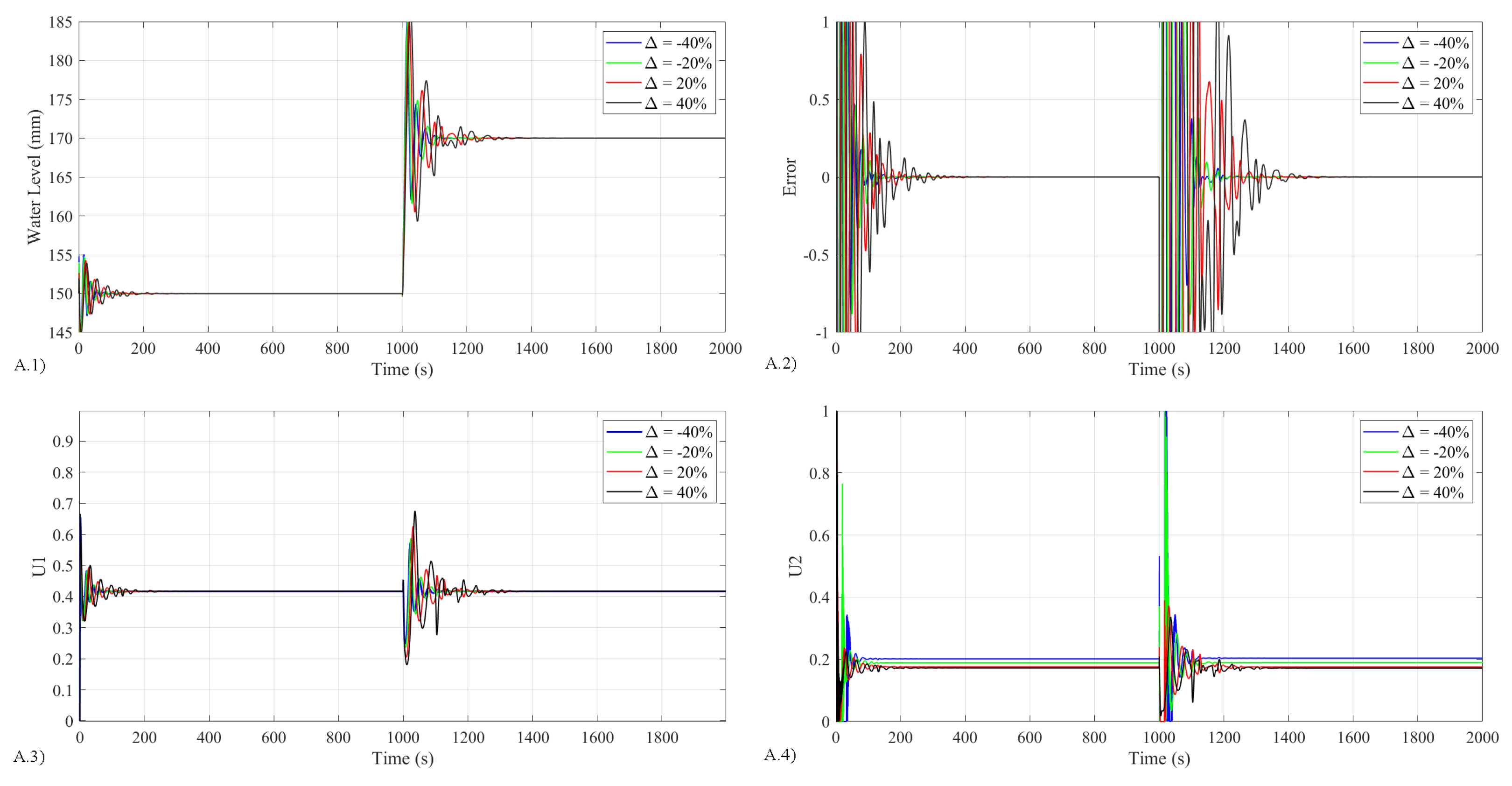
The purpose of this section is to assess the robustness of the proposed controller under both conditions of unknown disturbances and system parametric uncertainties. Simulation results of the closed-loop system response are illustrated in Figure 8 and Figure 9. In the hydrocyclone deoiling system, some parameters are susceptible to change due to changes in water level and PDR, as well as due to unknown dynamics of the system. The system (1) with parameter uncertainties is described as follows:

$$\dot{x}\left(t\right)=\tilde{A}x\left(t\right)+\tilde{B}u\left(t\right)+B_d{d}_j\left(t\right)$$

(57)

where $\tilde{A}=A+\Delta A$, and $\tilde{B}=B+\Delta B$ are system input matrices with bounded parameter uncertainties as well as unknown disturbances $d_j\left(t\right)$, respectively. Here, the deviation from the nominal value is considered within $\pm 20$ and $\pm 40$ percentages, respectively.

Figure 8 shows the system’s response with respect to parameter uncertainties and unknown disturbances when step changes occur in the reference model at 1000 s for S1-C1. The results presented by this figure include water level output, error signal, and control effort signals. As can be seen, the proposed robust MV-MRAC achieves the desired control objectives, including asymptotic output tracking and convergence of error signals to zero across various scenarios of parameter uncertainty and disturbance. Moreover, both control effort signals, shown in A.3 and A.4, are in a desirable range. It is established that the proposed MV-MRAC exhibits robustness even in the presence of varying parametric uncertainties and unknown disturbances.

A summary of the results for controlling the PDR signal related to S1-C2 can be found in Figure 9. As shown in the figure, the effectiveness of the proposed controller has been confirmed and the control objectives have been met for PDR control as well. In addition,

Table 1. MAE index obtained from the Optimized-PI and MV-MRAC for scenario 1.

	S1-C1		S1-C2
	Optimized-PI	MV-MRAC	Optimized-PI	MV-MRAC
$\Delta =-0.4$	1.1930	0.3159	1.0293	0.1301
$\Delta =-0.2$	1.1726	0.3470	0.9734	0.1321
$\Delta =+0.2$	1.1514	0.4653	0.8117	0.1478
$\Delta =+0.4$	1.1899	0.5906	0.7031	0.1622

and

Table 2. MAE index obtained from the Optimized-PI and MV-MRAC for scenario 2.

	S2-C1		S2-C2
	Optimized-PI	MV-MRAC	Optimized-PI	MV-MRAC
$\Delta =-0.4$	1.0353	0.3250	1.0293	0.3128
$\Delta =-0.2$	0.9803	0.2003	0.9734	0.2874
$\Delta =+0.2$	0.8222	0.2843	0.8117	0.2714
$\Delta =+0.4$	0.7184	0.3049	0.7031	0.2904

provide detailed information regarding the MAE index obtained from optimized PI and MV-MRAC for different uncertainty levels. As can be seen from this table, the proposed MV-MRAC performs better than the optimized PI under different system parametric uncertainties in all scenarios and cases.

A statistical analysis has been conducted to evaluate the reliability and precision of the closed-loop system. For this purpose, a series of 20 different simulations have been executed for each scenario and each case, incorporating the variability and uncertainty inherent in the system parameters. The mean value of the MAE index, the standard deviation, the standard error of the mean, and the 95% confidence interval obtained by this analysis are presented in

Table 3. Statistical analysis of reliability and precision for scenario 1.

	S1-C1		S1-C2
	Optimized-PI	MV-MRAC	Optimized-PI	MV-MRAC
Mean	1.167	0.431	0.876	0.137
Standard Deviation	0.040	0.052	0.070	0.016
Standard Error of the Mean	0.009	0.012	0.016	0.004
95% Confidence Interval	(1.14, 1.18)	(0.40, 0.45)	(0.84, 0.91)	(0.13, 0.14)

and

Table 4. Statistical analysis of reliability and precision for scenario 2.

	S2-C1		S2-C2
	Optimized-PI	MV-MRAC	Optimized-PI	MV-MRAC
Mean	0.879	0.278	0.880	0.291
Standard Deviation	0.070	0.025	0.073	0.015
Standard Error of the Mean	0.016	0.006	0.016	0.003
95% Confidence Interval	(0.84, 0.91)	(0.26, 0.29)	(0.84, 0.91)	(0.28, 0.29)

.

5.4.3. Results of the Adaptation Rate optimization

The results regarding the proposed optimization problem are presented and evaluated in this section. As mentioned before, given that the proposed problem is defined as an NLP optimization problem, the TLBO algorithm is carried out to solve it. Because of the uncertain behavior of a metaheuristic algorithm, it should be run multiple times with the aim of achieving the best result. After executing the problem in different epochs and finding the optimal solution for each epoch, the best solution $\mathrm{X}{1}_{MV-MRAC}^{*}$ has been considered for the proposed controller, and the second optimal solution among the obtained results is also considered and denoted by $\mathrm{X}{2}_{MV-MRAC}^{*}$. Respectively, $\mathrm{X}{1}_{PI}^{*}$ and $\mathrm{X}{2}_{PI}^{*}$ demonstrate the first and second optimal solutions for the optimized PI controller system. The results obtained for the closed-loop system regarding tracking the water level for the nominal system are pictured in Figure 10.

6. Conclusions

In this paper, a robust MV-MRAC solution based on output feedback is proposed and tested on a water treatment system, with the goal of improving output tracking goals in the presence of uncertain disturbances and system parameter uncertainty. The proposed control scheme is developed by using LDS decomposition to relax the conditions on the high-frequency gain. Moreover, the estimation error is employed to improve the controller’s tracking performance by applying the low-pass filters to the system’s input and output signals. To evaluate the proposed closed-loop system, two different scenarios are assumed by considering two different cases for each of them in the simulation section. The robustness of the proposed MV-MRAC controller is evaluated with respect to unknown disturbances and compared to the performance of the optimized PI controller. Simulation outcomes show that the proposed robust MV-MRAC method outperforms the optimized PI controller in terms of asymptotically tracking the reference. Moreover, a statistical analysis is employed for the reliability and precision of the closed-loop system through 20 simulations per scenario, accounting for parameter variability and uncertainty. The simulation results show that the proposed method perfectly rejects the uncertain disturbances and guarantees global stability through real-time control parameter adaptation. In S1-C1 and S2-C1, the proposed method reduces the mean value of MAE by 63% and 68%, respectively, compared to the Optimized-PI controller.

References

- Durdevic, P.; Yang, Z. Application of H∞ Robust Control on a Scaled Offshore Oil and Gas De-Oiling Facility. Energies 2018, 11, 287. [Google Scholar] [CrossRef]
- Skogestad, S.; Postlethwaite, I. Multivariable Feedback Control: Analysis and Design; John Wiley & Sons, Inc.: Hoboken, NJ, USA, 2005. [Google Scholar]
- Hansen, L.; Durdevic, P.; Jepsen, K.L.; Yang, Z. Plant-wide Optimal Control of an Offshore De-oiling Process Using MPC Technique. IFAC-PapersOnLine 2018, 51, 144–150. [Google Scholar] [CrossRef]
- KG, M.V.; Holden, C.; Skogestad, S. A First-Principles Approach for Control-Oriented Modeling of De-oiling Hydrocyclones. Ind. Eng. Chem. Res. 2020, 59, 18937–18950. [Google Scholar] [CrossRef]
- Jespersen, S.; Yang, Z. Performance Evaluation of a De-oiling Process Controlled by PID, H∞ and MPC. In Proceedings of the IECON 2021—47th Annual Conference of the IEEE Industrial Electronics Society, Toronto, ON, Canada, 10 November 2021; pp. 1–6. [Google Scholar] [CrossRef]
- Tao, G. Adaptive Control Design and Analysis; John Wiley & Sons, Ltd.: Hoboken, NJ, USA, 2003. [Google Scholar] [CrossRef]
- Pedersen, S. Plant-Wide Anti-Slug Control for Offshore Oil and Gas Processes. Ph.D. Thesis, Aalborg University, Aalborg, Denmark, 2016. [Google Scholar] [CrossRef]
- Jahanshahi, E.; Skogestad, S. Nonlinear control solutions to prevent slugging flow in offshore oil production. J. Process Control 2017, 54, 138–151. [Google Scholar] [CrossRef]
- Li, S.; Durdevic, P.; Yang, Z. Model-free H∞ tracking control for de-oiling hydrocyclone systems via off-policy reinforcement learning. Automatica 2021, 133, 109862. [Google Scholar] [CrossRef]
- Vallabhan KG, M.; Holden, C.; Skogestad, S. Deoiling Hydrocyclones: An Experimental Study of Novel Control Schemes. SPE Prod. Oper. 2022, 37, 462–474. [Google Scholar] [CrossRef]
- Diehl, F.C.; Almeida, C.S.; Anzai, T.K.; Gerevini, G.; Neto, S.S.; Von Meien, O.F.; Campos, M.C.; Farenzena, M.; Trierweiler, J.O. Oil production increase in unstable gas lift systems through nonlinear model predictive control. J. Process Control 2018, 69, 58–69. [Google Scholar] [CrossRef]
- Kashani, M.; Jespersen, S.; Yang, Z. Robust Multivariable Model Reference Adaptive State Feedback Output Tracking Control: An Offshore Produced Water Treatment Case Study. In Proceedings of the 2023 9th International Conference on Control, Decision and Information Technologies (CoDIT), Rome, Italy, 24 October 2023; pp. 2317–2324. [Google Scholar] [CrossRef]
- Song, G. A New Framework of Model Reference Adaptive Control Partial-State Feedback Designs and Applications. Ph.D. Thesis, University of Virginia, Charlottesville, VA, USA, 2019. [Google Scholar]
- Song, G.; Tao, G. Partial-state feedback multivariable MRAC and reduced-order designs. Automatica 2021, 129, 109622. [Google Scholar] [CrossRef]
- Wen, L.; Tao, G.; Liu, Y. Multivariable adaptive output rejection of unmatched input disturbances. Int. J. Adapt. Control Signal Process. 2016, 30, 1203–1227. [Google Scholar] [CrossRef]
- Selfridge, J.M.; Tao, G. Multivariable output feedback MRAC for a quadrotor UAV. In Proceedings of the 2016 American Control Conference (ACC), Boston, MA, USA, 1 August 2016; pp. 492–499. [Google Scholar] [CrossRef]
- Bagherpoor, H.; Salmasi, F.R. Robust model reference adaptive output feedback tracking for uncertain linear systems with actuator fault based on reinforced dead-zone modification. ISA Trans. 2015, 57, 51–56. [Google Scholar] [CrossRef] [PubMed]
- Hua, C.C.; Leng, J.; Guan, X.P. Decentralized MRAC for large-scale interconnected systems with time-varying delays and applications to chemical reactor systems. J. Process Control 2012, 22, 1985–1996. [Google Scholar] [CrossRef]
- Narendra, K.S.; Annaswamy, A.M. Stable Adaptive Systems; Dover Publications: Mineola, NY, USA, 2012; Available online: https://books.google.co.uk/books?id=CRJhmsAHCUcC (accessed on 22 February 2024).
- Guo, J.; Liu, Y.; Tao, G. A multivariable MRAC design using state feedback for linearized aircraft models with damage. In Proceedings of the 2010 American Control Conference, Baltimore, MD, USA, 30 June–2 July 2010; pp. 2095–2100. [Google Scholar] [CrossRef]
- Lan, W.; Chen, B.M.; Ding, Z. Adaptive estimation and rejection of unknown sinusoidal disturbances through measurement feedback for a class of non-minimum phase non-linear MIMO systems. Int. J. Adapt. Control Signal Process. 2006, 20, 77–97. [Google Scholar] [CrossRef]
- Wolovich, W.A.; Falb, P.L. Invariants and Canonical Forms under Dynamic Compensation. SIAM J. Control Optim. 1976, 14, 996–1008. [Google Scholar] [CrossRef]
- Wang, C.; Wen, C.; Zhang, X.; Huang, J. Output-feedback adaptive control for a class of MIMO nonlinear systems with actuator and sensor faults. J. Frankl. Inst. 2020, 357, 7962–7982. [Google Scholar] [CrossRef]
- Liu, Y.; Tao, G. An Adaptive Disturbance Rejection Algorithm for MIMO Systems with An Aircraft Flight Control Application. In AIAA Guidance, Navigation and Control Conference and Exhibit; American Institute of Aeronautics and Astronautics: Reston, VA, USA, 2007. [Google Scholar] [CrossRef]
- Rao, R.; Savsani, V.; Vakharia, D. Teaching—Learning-based optimization: A novel method for constrained mechanical design optimization problems. Comput.-Aided Des. 2011, 43, 303–315. [Google Scholar] [CrossRef]
- Yang, Z.; Juhl, M.; Løhndorf, B. On the innovation of level control of an offshore three-phase separator. In Proceedings of the 2010 IEEE International Conference on Mechatronics and Automation, Xi’an, China, 7 October 2010; pp. 1348–1353. [Google Scholar] [CrossRef]
Figure 1.
Simplified P&IDof the deoiling system under consideration consisting of a TPGS, a hydrocyclone, and their relevant control loops.
Figure 2.
Proposed robust MRAC structure and parameterization.
Figure 3.
Schematic view of the simulation scenario categorization.
Figure 4.
Results obtained for S1-C1 and with system disturbance; (A.1) PDR output, (A.2) Adaptation parameters, (A.3) The first control effort, (A.4) The second control effort.
Figure 5.
Results obtained for S1-C2 and with system disturbance; (A.1) PDR output, (A.2) Adaptation parameters, (A.3) The first control effort, (A.4) The second control effort.
Figure 6.
Results obtained for S2-C1 and with system disturbance; (A.1) Water level output, (A.2) Adaptation parameters, (A.3) The first control effort, (A.4) The second control effort.
Figure 7.
Results obtained for S2-C2 and with system disturbance; (A.1) PDR output, (A.2) Adaptation parameters, (A.3) The first control effort, (A.4) The second control effort.
Figure 8.
Results obtained for S1-C1 and with system disturbance and parametric uncertainty; (A.1) Water level output, (A.2) Error signals, (A.3) The first control effort, (A.4) The second control effort.
Figure 9.
Results obtained for S1-C2 and with system disturbance and parametric uncertainty; (A.1) PDR output, (A.2) Error signals, (A.3) The first control effort, (A.4) The second control effort.
Figure 10.
Results of water level obtained for optimized controller for nominal system.