Article

Research on the Influence of Lateral Force and Pressure Fluctuation on the Stability of a Rotary Energy Recovery Device in the Desalination System

1
Ocean College, Zhejiang University, Zhoushan 316021, China
2
Yangjiang Offshore Wind Energy Laboratory, Yangjiang 529500, China
*
Author to whom correspondence should be addressed.
Water 2024, 16(6), 823; https://doi.org/10.3390/w16060823
Submission received: 14 February 2024 / Revised: 8 March 2024 / Accepted: 9 March 2024 / Published: 12 March 2024
(This article belongs to the Special Issue CFD in Fluid Machinery Design and Optimization)

Abstract

:
The rotary energy recovery device (RERD) plays an important role in reverse osmosis (RO) desalination; however, few investigations on the formation and influence of lateral force on the RERD rotor have been published. The transient characteristics of lateral force and its relationship with pressure distribution and fluctuation in the clearance were analyzed via computational fluid dynamics (CFD) simulation. The clearance pressure distribution and lateral force were quantified under different working conditions. The eccentricity of the rotor, resistance torque and decrease in the rotary speed due to the lateral force were simulated and they were found to change with flow rate and pressure of high-pressure outlet (PHO). A new rotary speed prediction method including the effect of PHO was developed. With the increasing flow rate or PHO, the stability of RERD declined. A design optimization direction was proposed. The variation trends of rotary speed, pressure in the clearance and its fluctuation were verified through experiment. This research provides an explanation why in practice the rotary speed decreases with increasing pressure. The conclusions obtained herein can be of great significance for future research on improving the stability and lifespan and reducing the maintenance consumption of RERD.

Graphical Abstract

1. Introduction

Water shortage has become a worldwide problem [1]. Global water use has been growing at an annual rate of 1% over the past 40 years and will continue to grow until 2050. Ten percent of the global population is living in countries with high or severe water scarcity [2]. The shortage of fresh water is causing the world water security great challenges [3]. Climate change, population growth, pollution and increase in industrial water use are all causes of this problem, while uneven distribution of water resources makes the problem worse in some regions [4,5,6,7]. To alleviate this crisis, seawater desalination technology, which is considered to be one of the most economical fresh water preparation methods due to abundant seawater resources, has become the focus of research [8,9]. Reverse osmosis (RO), with low energy consumption and health risks, is the most widely used seawater desalination technology [10,11]. Reparation processes and performance improvement of membrane, design and computational fluid dynamics (CFD) analysis of energy recovery devices (ERDs) have been the research focuses of the RO desalination field [12,13] in recent years.
The ERD (with the ability to recover energy from brine for pressurizing seawater to reduce the consumption of desalination) has become the key equipment of the RO system; it is also widely used in other water treatment fields such as underground brine and water distribution [14]. ERDs can be classified into turbine ERD and isobaric ERD. When the isobaric ERD is working, the energy of brine directly transforms to the seawater without any intermediate steps of energy conversion (called the positive displacement principle). Therefore, the isobaric ERD consumes less energy than the turbine ERD, with an intermediate energy conversion turbine step. Moreover, isobaric ERDs can be classified into a piston-type ERD (also called valve-type ERD) and a rotary energy recovery device (RERD). The inflow and outflow of brine and seawater are controlled by valves in the piston-type ERD, while a rotor controls the liquids flowing in and out of the RERD. The RERD (with its small size and low maintenance) performs well in large-scale reverse osmosis plants [15,16,17,18]. The RERD used in the RO system is shown in Figure 1.
The RERD contains two end covers, an outer sleeve and a rotor with several channels (as shown in Figure 2). The device uses high-pressure brine rejected by the RO membrane to pressurize seawater through contacting each other directly in the rotor channels to save the power of the high-pressure pump. The high-pressure brine transforms pressure energy to the low-pressure seawater in the channels of the RERD and then the seawater becomes high pressure and flows out of the RERD to the membrane. The inflow and outflow of brine and seawater are controlled by the rotation of the rotor. Meanwhile, the rotor is driven by the inflow fluids impinging on the channel wall, without an external motor to save electric energy. There is a clearance (as shown in Figure 3) between the rotor and sleeve, where liquid film is formed to support and lubricate the rotor [19]. Because of these structures, RERDs can be affected by various factors, including the driving torque and resistance torque, respectively, acting on the inner walls of the channels and the outer walls of the rotor, mixing in the channels between brine and seawater, and the lateral force on the rotor caused by the even pressure distribution of the liquid in the circular clearance.
The performance parameters of RERD have been studied extensively in past years. Xu et al. [20] carried out numerical simulation and experimental research on the static pressure support of the adjustable liquid film to the rotor. Wu et al. [21] added grooves to the end-cover structure to reduce the resistance torque of the rotor and improve the energy recovery efficiency. Jiao et al. [22] researched the hydrodynamics of RERD and analyzed the influence of working conditions on the rotor torques through simulation and experiment. Xu et al. [23] studied the rotary speed of the hydraulic self-driven rotor and its influencing factors, while Huang et al. [24] established the method of speed prediction by flow rate. Mixing occurs in the channels because there is no physical barrier between brine and seawater [25]. Zhou et al. [26] explored the factors affecting the formation of the mixing zone in the rotor channels. Liu et al. [27] observed the flow field and mixing phenomenon in the channels through the PIV visualization method. Li et al. [28] used a kind of inclined channel to reduce the mixing rate of RERD. Xu et al. [29] researched the working conditions influencing the mixing rate of the servomotor-driven RERD via CFD simulation, while Ye et al. [30] investigated that of a hydraulic self-driven RERD and the effect of angles in end covers. Ye et al. [31] and Sun et al. [32] designed a rotary vane RERD and a new swash plate-plunger RERD, respectively. These studies focused on energy recovery efficiency, rotary speed and mixing of RERD. The studies mentioned above can be classified according to Table 1.
Few reports were found regarding the radial force (called lateral force in this paper) acting on the rotor of RERD. Lateral force and its effects on the stability of the RERD and the desalination process were found through problems occurring in the actual operation. According to previous studies, the rotary speed of RERD depended on the flow rate. However, it was found in practice that, when the pressure at the high-pressure end cover (PHO) increased, the rotary speed began to decrease. It was also found in the Liuheng desalination plant in Zhoushan, China that the more unstable devices with larger fluctuations in rotary speed affected by lateral force required more frequent maintenance. In simulation, it was discovered that the unbalanced lateral force acting on the outer wall of the rotor through the liquid in the circular clearance in the direction perpendicular to the rotation axis was too large. According to the experience of the pump and fluid-excited vibration research, this force might affect rotary speed via changing the resistance torque of the rotor; meanwhile, its fluctuation can influence the stability of the rotor [33,34]. Therefore, the investigation of lateral force, pressure fluctuation and their effects on the stability of RERD in practice is of great significance to improve the stability of the RO desalination process through finding the method to make the rotary speed more stable, less affected by operating pressure and with less fluctuation. This method can be used for reducing the maintenance frequency and consumption of the rotor and cost of the plant. From the above review, it can be found that these important questions that should be taken seriously in the RERD field were ignored in past research. Herein, we discuss the details of lateral force, pressure distribution, fluctuation and stability.

2. Theoretical and Simulation Methodologies

2.1. Formation and Influence of Lateral Force

The outer wall of the rotor is subjected to the pressure of the liquid in the circular clearance. As the device is divided into two zones of high- and low-pressure areas, the pressure distribution on the two ends of the rotor becomes uneven. Therefore, after the liquid in the end-cover clearance leaks into the circular clearance, the pressure distribution around the outer wall of the rotor is not uniform, which makes an asymmetry on the liquid force on the bilateral wall surfaces of rotor central shaft, and the direction of resultant force is perpendicular to the central axis and points to the horizontal direction. The force is called lateral force in this paper. Due to the influence of rotor rotation, the pressure of each point in circular clearance will fluctuate with time, and this pressure fluctuation will result in the fluctuation of the lateral force. It can be inferred that there is a direct connection between lateral force magnitude and the pressure distribution around the rotor outer wall (the circumference of circular clearance) according to the generating mechanism of lateral force. Meanwhile, the transient change characteristics of lateral force should be of great relevance with the fluctuation of pressure in this clearance.
The definition of lateral force direction is shown in Figure 4. A rectangular coordinate system is established on the rotor section (the rotor rotates clockwise). The right side of the Y-axis is the zone connected to the high-pressure side of the end cover, called the high-pressure area, and the left side is the low-pressure area.
The rotor produces an eccentric motion by lateral force, and the variation of clearance thickness changes the resistance torque of the rotor formed by the liquid film. The thickness of clearance is very small, usually 0.02 mm, and the flow rate inside it is no bigger than 20 m/s. Therefore, the Reynolds number is usually no higher than 2000, and the laminar flow is the main flow. According to Newton’s theory of inner friction, end-cover and circular clearance can be unfolded, while the liquid film can be, respectively, regarded as the flow between two circular/rectangular parallel plates. The wall surface of the rotor will move at a corresponding linear speed while the sleeve wall surface is fixed, and velocity gradient will occur between the parallel plates. Taking each place in the clearance as two infinitesimal parallel plates, the shearing stress is calculated on each small infinitesimal wall surface, and the theoretical formula of resistance torque suffered by the rotor after using surface integral is obtained [23,24]:
M R = π 2 μ N ( Lr 3 15 c 1 + r 4 r 4 30 c 2 )
where N is the rotary speed of rotor (rpm); μ is the hydrodynamic viscosity (N·s/m2); L is the length of rotor (m), r and r’ are the outer wall radius of rotor and the center hole radius of rotor (m), respectively; c1 and c2 are the thickness of circular clearance and the end-cover clearance, respectively (m). The part before the plus sign in parentheses is the circular clearance resistance term, while that after the plus sign is end-cover clearance resistance. When the thickness of circular or end-cover clearance decreases, the flowing velocity gradient in the clearance becomes steeper and the liquid resistance acting on the lateral outer wall or the end face of the rotor will increase, which reduces the rotary speed. The resistance torque also decreases with the rotary speed, forming a negative feedback balance. The formula is suitable for the ideal case where the rotor is not eccentric. However, in the study of lateral force, hereafter, it is found that the rotor will move eccentrically under the impact of lateral force, and the thickness of a single side of liquid film will change to increase the resistance torque, which leads the annular resistance in the formula to increase to reduce the rotary speed. Therefore, the experimental speed is a little lower than the theoretical speed during previous experiments operated by researchers.

2.2. Computational Fluid Dynamics Model and Control Equation

In this paper, STARCCM+ was used to numerically solve the model, and the unsteady and incompressible three-dimensional Reynolds mean Navier–Stokes equation (RANS) was solved. The heat transfer during the process of operation was ignored because there was no heat transfer in the operation of the device. The continuity equation and momentum equation can be described as [35]:
u x + v y + w z = 0
( ρ u i ) t + ( ρ u i u j ) x j = p x i + τ ij x j + ρ g i ρ u i ¯ u j ¯ x j
where ρ is fluid density (kg/m3), ρgi is the volume force in the i direction (N/m3), τ is the viscous stress tensor (N/m2), and ρ u i ¯ u j ¯ is Reynolds stress (N/m2). The Reynolds stress term makes the system of equations no longer closed and cannot be solved directly. In order to solve this problem, various turbulence calculation models are introduced, which can be divided into a Reynolds stress model (RSM) and a vorticity viscosity model according to different assumptions of Reynolds stress terms. The eddy viscosity model is often used in engineering, which introduces turbulent viscosity to calculate Reynolds stress [35].
ρ u i u j = μ τ ( u i x j + u j x i ) 2 3 ρ k δ i j
k = 1 2 u i u j
where μτ denotes turbulent viscosity and k means turbulent kinetic energy.
According to the number of differential equations determining μτ, the eddy viscosity model can be divided into a zero-equation model, a one-equation model and a two-equation model. In engineering practice, two-equation models are widely used, including the standard k-ε model, RNG k-ε model and realizable k-ε model. According to the research results of Liu, the numerical simulation results using the realizable k-ε turbulence model are in nice agreement with the PIV experimental data of a rotary energy recovery device, which can be used to analyze the detailed information of flow characteristics in the rotor channels of the RERD. The flow in the clearance is mainly laminar flow. According to the conclusions of Sparrow et al. [36], for the flow simulation that contains independent laminar flow with turbulence flow in other areas, in the independent laminar flow area, due to the geometric factor of the device, when Re < 370, the standard k-ε model has a large error in calculating laminar viscosity by turbulent viscosity. When Re is higher than this value for other models, this error is small and acceptable. Therefore, for the fluid domain studied in this paper, where the laminar flow only exists in the clearance with the Re larger than 500 and in the other parts there is turbulence flow, the realizable k-ε turbulence model can be used to calculate the simulation. Therefore, the realizable k-ε turbulence model was adopted in this paper.

2.3. Simulation Scheme

The flow domain model of RERD was drawn in NX UG (ver. 10.0) (shown as Figure 5). It contains 4 end covers, 24 rotor channels and 2 clearance parts. The length of the channel is 190 mm and the thickness of clearance is 0.02 mm (the same as the device in the experiment). There are 36 sampling points arranged uniformly around the circular clearance wall, forming a sampling point circumference. Three such circumferences are evenly distributed in the rotor axis direction. Circumference N-1 is at the middle height of the rotor, while N-3 is on the end face and N-2 is on the middle line between N-1 and N-3 (N here represents the circular number of the sampling point, not the rotary speed).
The mesh model was created in Ansys ICEM CFD (ver. 17.2), as shown as Figure 6. The structural grid was used for the rotor channels and clearance parts with 6 boundary layers, while the unstructured grid was used for the irregular part of the end-cover structure. All the meshes were combined in the simulation software STARCCM+ (ver. 16.02.009-R8). The total number of meshes was over 2,600,000, and the minimum orthogonal quality of the whole mass was 0.4.
The end-cover outlets were set as pressure outlets, while the inlets were velocity inlets to make the calculation easy to converge. Inflow velocity was calculated by the flow rate and inlet area. Herein, the flow in the clearance was mainly focused and the mixing problem in the rotor channels was not considered; therefore, the fluid was set as water without considering the component transport model. The contact surfaces between the end-cover down face and between the end-cover clearance, the end-cover clearance and the end face of the rotor channels were set as interfaces to connect the entire fluid domain according to the actual flow situation, and the other surfaces were set as the wall surface. The sliding mesh method was adopted for the transient calculation of the rotor rotation. The fluid domain of the rotor channels was set as the rotating region, and the inner surface of the clearance liquid film connecting with the rotor was set as the rotating wall with the same speed as the rotor to comply with Newton’s internal friction theory. The other walls and areas were set as static surfaces and regions, and wall enhance treatment was used. The first-order upwind scheme was used to discretely calculate the turbulent kinetic energy and turbulent dissipation rate. The second-order upwind scheme was used to calculate the momentum equation. To reduce the residuals, the maximum number of internal iteration steps was set to 20. The results of the transient calculation negligibly changed when the time step was lower than the time when the rotor rotated 1°, therefore the time step was set as that. The residual standard of convergence was set to 1 × 10⁻⁴ and, when the residual values were reached, the simulation results were considered to be stable. Then, the data during at least one rotation cycle of the rotor were taken for monitoring. The monitors were set to record resistance torque, lateral force in each direction and the pressure of 108 sampling points on the inner wall of the circular clearance. The power spectral density curves of lateral force and pressure fluctuation in frequency domain were generated by fast Fourier transform (FFT) (via Hann window function) in the software STARCCM+ mentioned above. The reliability of the computation mesh was verified by a mesh number independence check (Table 2).

3. Simulation Results and Discussion

3.1. Lateral Force, Pressure Distribution and Fluctuation When Rotor Was Non-Eccentric

First, the initial position of the rotor without eccentricity was calculated. The working condition was set with a flow rate of 70 m3/h and a pressure of 6 MPa, while the estimated rotary speed of the rotor applied in this paper was 700 rpm (according to Huang’s [24] speed prediction method). The lateral force (the lateral outer wall of the rotor was the only component that the lateral force acted on) in the X and Y directions on the rotor at this speed was monitored, and the sampling duration was within one rotating cycle of the rotor, as shown in Figure 7.
As shown in the figure, the lateral force in the X direction pointed at the negative direction of the X-axis, and the magnitude fluctuated between −140 kN and −130 kN. The direction and magnitude of the lateral force in the Y direction fluctuated between the positive and negative direction of the Y-axis around zero, and the fluctuation range was bigger than in the X direction. No matter the lateral force in the X or Y direction, they all had similar periodical laws of fluctuation, which meant there were 16 peak values and 16 valley values in the curve of lateral force within 1 rotating cycle. The lateral force fluctuated 16 times when the rotor rotated 1 cycle, and there were 8 higher peaks and 8 lower valleys, which were arranged in order. The valley values were the same, and the higher and lower peak-valley values of the lateral force in the X and Y directions almost emerged at the same moment. This fluctuation cycle of the lateral force coincided with the number of rotor channels. In the device applied in this paper, 16 outer channels and 8 inner channels existed in 1 rotor, and 2 outer channels and 1 inner channel formed a channel group (total 8 groups). Therefore, it can be inferred that the transient fluctuation characteristics of the lateral force had a certain relation with the position of the rotor channel. To research the relations between them, the relative position diagram of the rotor channels and the inflow end cover was shown when four peak and valley values emerged within a smaller fluctuation cycle of the lateral force (in Section A, Figure 7, there are two pairs of peak and valley values (higher peak a and lower peak c, lower valley b and higher valley d)).
At position a in Figure 8, one group of rotor channel Ⅰ plunged into the high-pressure end cover area. At that moment, one side of the inner channel ⅰ and outer channel i-i of this group was tangent to the arc edge of the end cover, corresponding to the higher peak emerging in Figure 7. Meanwhile, this group of channels changed from no liquid flowing in or out to high-pressure seawater flowing into two channels at the same time. At position b, part of the inner channel ⅰ had already passed inside the inflow area, most of the outer channel i-i had passed inside the inflow area and the lower valley b of the lateral force emerged. At position c, part of the inner channel ⅰ was still out of the inflow area, meanwhile one side of the outer channel i-ⅱ was tangent to the arc edge of the end cover and starting to go into the inflow area. At this moment, the sub-peak c of the lateral force emerged and one channel of this group changed from no liquid flowing in or out to seawater beginning to flow in. At the last position d, both other sides of inner channel i and outer channel i-ii were tangent to the arc of the end cover, had fully passed into the inflow area and the sub-lower valley d of the lateral force emerged. Then, the next channel group rotated until reaching position a of channel group I, the magnitude of the lateral force came to the next higher peak and the cycles repeated. As there were 8 groups per channel, such a cycle would repeat 8 times within 1 turn of rotation, which meant the magnitude of the lateral force had 16 pairs of peaks and valleys. The position of the channel group on the opposite side of the center of the circle relative to the low-pressure inflow area behaved the same as above because the rotor had a central symmetry structure. It can be seen from the above analysis that, when one inner channel and one outer channel of one channel group plunged into the outflow area at the same time (the moment when the edges of two channels started to cut the inflowing fluid), the lateral force reached the highest peak value. And when the edge of only one channel started to cut the inflowing fluid, the lateral force reached the sub-highest peak value. Moreover, the valley values of the two lateral forces corresponded to the time that the channels were completely in the outflow area and the edges no longer cut the inflowing fluid. It was believed that the abrupt change of the inflow speed at the beginning of the “cut” caused the pressure to reach the peak, and then also caused the lateral force to reach the peak. The number of channels on the rotor was the number of peaks of the lateral force and pressure within one turn of rotation, therefore forming the periodical pressure fluctuation, which caused the periodical fluctuation of the lateral force.
Figure 9 shows the power spectral density (PSD) curves in the frequency domain of the X and Y direction; their main frequency was 185 Hz, 16 times the rotation frequency (about 11.7 Hz, as the rotary speed was 700 rpm) of the rotor, while the secondary frequency was 95 Hz, 8 times the rotation frequency of the rotor. It accorded with the fluctuation curve of the amplitude of the lateral force in the time domain, and also accorded with the numbers of rotor channels mentioned above. In addition, the amplitude of the power spectral density at the main frequency (PSDM) of the lateral force in the Y direction was much higher than in the X direction. It was confirmed that the lateral force in the Y direction had a larger fluctuation amplitude than in the X direction. The reason for this phenomenon could be that the lateral force in the X direction was much greater than in the Y direction and the influence of pressure fluctuation was less obvious, while the lateral force in the Y direction was small, so it was more affected by the pressure fluctuation. The PSDM of the lateral force in the X and Y directions were 4.5 × 10⁵ and 1.1 × 10⁷ N2/Hz, respectively.
In order to define the resultant force of the lateral force and its fluctuation range more conveniently, the lateral force could be regarded as the superposition of a constant force and a changing pulse force. The constant force was represented by the mean value of the lateral force, and the standard deviation of the lateral force was used to show the fluctuation amplitude of the pulse force (called “excitation force” in this paper); the formula is as follows:
F 0 = i = 1 n F i / n
f = 1 n i = 1 n ( F i F 0 ) 2
where F0 is the mean value of the reluctant force of the lateral force, Fi is the reluctant force magnitude of the lateral force every time, n is the sampling times and f is the fluctuation amplitude of the lateral force measured by standard deviation (excitation force) with the same unit as the lateral force. According to the above formulas, the constant force and the excitation force of the resultant lateral force under this working condition were 139 kN and 1.97 kN, respectively.
Since the lateral force was generated by the uneven distribution of clearance pressure, the fluctuation of the pressure of the sampling points in the time domain should also have been consistent with the lateral force. The lateral force in the X direction was mostly related to the pressure of points 10-1 and 28-1, symmetrical distributing with the Y-axis on both sides, while the symmetrical distributing of points 1-3 and 19-3 with the X-axis and their pressure were related to the lateral force in the Y-direction. The pressure of the points are drawn in Figure 10.
It can be seen from the figures that the lateral forces in each direction fluctuated as the pressure of the points related to them. The time when the peak and valley values of the pressure fluctuation at each point and the reason were similar to those of the lateral force were caused by the different positions of the rotor channels (Figure 8). When the pressure difference between two symmetric points increased, the absolute value of the lateral force became larger. Moreover, the pressure of the points fluctuated with a frequency similar to the lateral force. Their main frequency was 185 Hz, 16 times the rotation frequency, while the secondary frequency was 95 Hz, 8 times the rotation frequency of the rotor. These points were taken as examples and the other sampling points exhibited similar fluctuation.
For the 36 pressure sampling points on the same circumference, the distribution angle was defined as Angle θ (Figure 4) between the line from the sampling point to the center of the circle and the +Y-axis. The curve between pressure and θ was drawn by the pressure from 36 sampling points, as shown in Figure 11. It can be seen that the curve showed an obvious sine form. Through fitting in origin, the fitting parameters of the sinusoidal curve obtained are shown in Figure 11, and the correlation reached 99.9%. According to the fitting parameters, the circular direction pressure distribution at the N-2 circumference was also close to the sinusoidal type, and the correlation coefficient reached 99.7%. Although the circular direction pressure distribution at the N-3 circumference also performed the same trend and periodicity, and the circular position of the maximum pressure value point was also the same, the fitting correlation coefficient was only 96.7%, and the curve form was between sine and square wave.
The main frequency of pressure fluctuation reflected the time of fluctuations of each point in one rotation cycle. The main frequencies of pressure at most of the sampling points were 185 Hz, 16 times the rotation frequency, and the reason was the same as the fluctuation of the lateral force. The amplitude of PSD reflected the intensity of pressure fluctuation at each point. Since the amplitudes of the PSDM of most points were much higher than that at other frequencies, the amplitude of PSDM was used to measure the fluctuation amplitude of a certain point in this period in order to reasonably simplify the operation.
In the vibration field, the root mean square (RMS) value of vibration was used to represent the average effective energy of a vibration signal, and the pressure fluctuation was seen as the result of fluid excitation. The RMS value was taken from the pressure at certain points in this period, and it had a similar function as PSDM. Figure 12 shows that the pressure RMS of each point from point 1-1 to point 36-1 was almost the same as the distribution trend of PSDM, so it was proven that the method of reflecting the amplitude of pressure fluctuation by PSDM at frequency domain was reliable.
Figure 13 displays the distribution of PSDM at each point of circumference N-1, N-2 and N-3. It can be seen that in the high- and low-pressure areas between point 5~15 and point 23~33, the pressure fluctuation amplitude of each point was low. The closer to the end face in the axial direction, the smaller the fluctuation amplitude was, of which the pressure fluctuation in the high pressure area was more intense. In the pressure transition area between the high- and low-pressure area, especially near point 3 and point 20, the pressure fluctuation amplitude increased greatly, and, the closer to the end face in the axial direction, the larger the pulsation amplitude was. PSDM at the end face was much higher than in the middle, meaning the pressure fluctuation of liquid in clearance was very intense around the pressure transition area and was gentle inside the high- and low-pressure area. The closer to the end face in the axial direction, the more obvious the phenomenon was. No obvious distribution fitting function was in the circular direction of the curve in Figure 13.

3.2. Lateral Force, Pressure Distribution and Fluctuation on Eccentric Rotor

The simulation results in this section were based on the actual lateral force and produced eccentric motion to which the rotor was subjected. To facilitate the monitoring of data of each sampling point and lateral force and to compare with the data under the non-eccentric condition, the center O’ of the eccentric rotor was taken as the coordinate origin (Figure 14), while the point O in the figure was the center of the rotor under non-eccentric condition (also the center of circle of the shaft section of the outer wall in the clearance). So, under the working conditions set like this, the origin parameters remained unchanged, such as the coordinates of each sampling point, the acted surface and direction of the force and torque, the surface of rotation (the outer wall of the rotor/the inner wall of the liquid film) and its speed, then the mesh was drawn with the same deformation in the opposite direction of the liquid film offset to the rotor. The simulation was calculated by this method, and the parameters and model selection were the same as before. The polar coordinate method was also adopted to represent the eccentricity by the displacement distance in the X and Y directions, as shown in Figure 14. The eccentric distance γ was the distance between O’ and O, and the deviation angle φ was the dip angle between the two-point line and the X-axis, and the eccentric of the rotor in horizontal direction was represented by these two parameters.
The stable position of the eccentric rotor under the flow rate of 70 m3/h and pressure of 6 MPa should be found. The stable position was determined as follows: (1) The position where forces on the rotor was almost balanced. It was hard to totally eliminate the lateral force, and it would change within a certain range and reduce to a very low level. It could be regarded as stable when reducing to the same order of magnitudes as the excitation force. (2) Torque was balanced on the rotor, meaning the driving torque was equal to the resistance torque. The rotary speed would reduce to a certain extent because the resistance torque increased after eccentricity. At the stable position under the working conditions mentioned above, the eccentric distance was 0.0135 mm and the deflection angle was 87°. Meanwhile, the lateral force in the X and Y direction at this time was 1980 N and 2010 N, and the reluctant lateral force was lower than 3 kN. The rotary speed reduced to 650 rpm and the actual central position of the rotor and the rotary speed fluctuated around these values.
Figure 15 showed the pressure cloud image in the clearance at this time. As φ approached 90°, the high-pressure and low-pressure concentration areas appeared above the X-axis and on the left and right sides of the Y-axis, respectively. Point 34-1 and point 3-1 were respectively their centers, offsetting the pressure differential of the low-pressure area on the left side and the high-pressure area on the right side, which caused the lateral force in the X direction to greatly decrease. The pressure of the sampling points on the outer wall of the rotor was taken to draw the pressure distribution curve (Figure 16) for each circular direction.
When the rotor was eccentric, the pressure in the original high- and low-pressure areas and pressure transition area changed greatly due to the influence of high- and low-pressure concentration areas caused by the narrowing of one side of the liquid film, especially on circumference N-1, where two centers of pressure concentration area (point 4-1, point 34-1) formed. The pressure that was originally in the transition area close to the high- and low-pressure area changed greatly, forming an extremely low pressure (0.56 MPa) and an extremely high pressure (6.69 MPa). The two pressure concentration areas appeared symmetrically on both sides of the narrowest part of the liquid film and were close to the narrowest part. If the rotation direction of the rotor was called the front, the high-pressure concentration area appeared behind the narrowest point of the liquid film, while the low-pressure concentration area was in front of the narrowest point of the liquid film. At this time, the narrowest point of the liquid film was almost on the +Y axis and the X coordinate was negative and very small so that the two pressure concentration areas were generated at the two positions that centered at points 4-1 and 34-1. The original high- and low-pressure points moved in the direction of the thickening liquid film, from point 10-1 and point 28-1 to point 14-1 and point 24-1, respectively. Because the centers of the pressure concentration areas were located on circumference N-1, the farther the distance in the axis direction was from the center and closer to the end face, the less influence on the pressure it had. For example, neither the extreme high pressure nor low pressure on circumference N-2 reached that of circumference N-1; the central positions and pressures of the original high- and low-pressure areas also changed little. The influence on circumference N-3 was minimal and it could be seen that the pressure distribution still maintained the original trend of first increasing, then decreasing and finally increasing again, but the overall dispersion degree of pressure was reduced. The mean values of the pressure of each point in one rotation cycle were taken and the standard deviations of such mean values of 36 points on the same circumference were calculated. The changes are shown in Table 3.
According to the pressure dispersion degree of the three circumferences, only the pressure distribution nonuniformity close to circumference N-1 had a small amplitude increase, and those on the other circumferences were reduced. Therefore, the pressure distribution nonuniformity in the clearance was greatly reduced as a whole and the lateral force was reduced from about 140 kN to the same level as the excitation force of 3 kN. The pressure distribution of circumference N-1 in the figure was very similar to the real pressure distribution of the centrifugal pump clearance [37], which also showed the reliability of the simulation in this paper.
Next, the frequency domain data of pressure fluctuation were analyzed. In the 108 sampling points, the main frequencies of the pressure fluctuation at most points were still 16 times (185 Hz) the rotation frequency (about 11.7 Hz, as the rotary speed was 700 rpm), and there were a few points with different main frequencies that were 8 times (95 Hz) or 32 times (370 Hz) the rotation frequency (Figure 17).
It can be seen from the pressure curve that points 29-3, 30-3 and 31-3 were the three points with the lowest pressure at the end face circumference, and these pressure values themselves were relatively low, more obviously affected by the inflow and outflow of the interface of end-cover clearance and circular clearance. The main frequency of the fluctuation was 370 Hz, twice the number of most of the sampling points.
Several points in the yellow circle were affected by the eccentric movement of the rotor, resulting in a high-pressure concentration area. Because the pressure became higher, the influence on pressure fluctuation by the rotor channel cutting the inflow liquid was reduced, as mentioned above. The fluctuation amplitude produced by a single channel cutting inflow liquid was much smaller than that of an inner channel and an outer channel cutting at the same time. Therefore, the main frequency was eight times the rotation frequency.
The distribution of PSDM on each circle is shown in Figure 18. The variation trend of the main frequency amplitude of pressure fluctuation in the circular direction was not much different from when the rotor was not eccentric. Meanwhile, the PSD amplitude of most positions decreased, and only the PSDM in the low-pressure concentration area increased, reaching a maximum of 7.5 × 10¹⁰ Pa2/Hz, which was more than double the maximum amplitude when the rotor was not eccentric.

3.3. The Factors Affecting the Rotor Eccentric Position and Stability

In this section, the rotor was simulated under different flow rates and PHO when the rotor was at the initial position without eccentricity. The pressure distribution curves and lateral forces were compared. Then, the rotor was simulated under the eccentric rotation influenced by the lateral force by changing the working condition parameters such as flow rate and PHO. The eccentric stable positions under each working condition were found and the formula corrections of the resistance torque and rotary speed influenced by the lateral force were obtained.
Firstly, the non-eccentric situations were simulated. The pressure distribution curves under different flow rates when PHO was set as 6 MPa and under different PHO when flow rate was set as 70 m3/h are displayed in Figure 19. The rotary speed related to the flow rate was set as Huang’s old model without eccentricity. When the flow rate changed, the dispersion of the curve became very slightly lower as the flow rate increased, while it decreased significantly when PHO decreased.
The lateral forces under the different working conditions mentioned above are drawn in Figure 20. It was found that the lateral force increased nearly linearly when PHO increased and decreased as the flow rate increased, but its decreasing trend was slight compared with its size. The lateral force exhibited a quadratic function relation with the flow rate. The fitting degree was good, with adjusted R2 over 0.99. It could be told from above that the rotor would be more eccentric when the flow rate decreased and PHO increased, similar to the change in lateral force.
Then, the simulation was calculated when the eccentric rotor was at the stable position and, herein, the lateral force was considered at a very low level near 0. The PHO was controlled constant and the flow rate was changed. The position and rotary speed of the eccentric rotor were adjusted for each working condition, so that the rotor reached a stable state. The stable position of the rotor was very close to the +Y-axis, and the deviation angle varied between 87° and 90°; meanwhile, the lateral force change caused by the deviation angle in this range was very small through the simulation test. The most influential factor was the eccentricity. Therefore, adjusting the eccentric distance γ was the main method of adjusting the position of the rotor. When the eccentric rotor was stable under different flow rates, the rotary speed and eccentric distance are shown in Table 4. It was found that the rotary speed decreased and the eccentric distance increased as the flow rate decreased.
The pressure distribution curve of each circle varied with the flow rate, as shown in Figure 21. The dispersion of the pressure distribution curve of circumference N-1 decreased as the flow rate increased. The pressure distribution of circumference N-2 was similar to that of N-1, and the pressure dispersion was lower than that of N-1. The pressure distribution trend of the N-3 circumference was not significantly affected by the flow rate and rotary speed, which was similar to when the rotor was not eccentric. It could be considered that the change of eccentric distance had little influence on the pressure distribution at the end-face circumference.
Then, the inflow rate was controlled constant and PHO was changed. The simulation was conducted under the working conditions when the rotor reached eccentric stabilization. It can be seen in Table 5 that the eccentric distance reduced as PHO decreased and the reducing speed gradually increased. The rotary speed increased, whereas the increasing speed gradually reduced until the rotary speed finally approached its predicted speed.
Figure 22 shows the circular pressure distribution curve in the clearance on eccentric stabilization with different PHO. When PHO decreased, the pressure in the clearance was reduced as a whole, the dispersion of pressure was also reduced and the non-uniform pressure distribution was reduced. When PHO decreased to 1 MPa, the pressure distribution curve flattened out, and the influence of the pressure concentration area was minimal.
The PSDM of the lateral force and the excitation force curve are shown in Figure 23, and it can be obtained from the figure that the PSDM of the lateral force in the Y direction and the excitation force of the resultant force both increased (the lateral force value in the X direction was small and fluctuated around 0; the lateral force in the Y direction greatly fluctuated). As the flow rate and PHO increased, the stability of the device reduced as the magnitude of the pressure fluctuation in the clearance increased.
It was found from the simulation results above that the eccentric distance and flow rate exhibited a clear relationship with PHO. The second-order fitted curved surface was obtained through their relations, as shown in Figure 24, and the adjusted R2 of the fitted surface was over 0.98. The fitted formula of the eccentric distance γ was (8). The calculation results of the efficiency factor (β) of Alford force under different working conditions are drawn in Figure S1. It increased as the flow rate increased and the PHO decreased.
γ = 3.79 0.16 Q + 6.14 P H O 0.024 Q P H O + 0.0011 Q 2 0.32 P H O 2
where Q is the inlet flow rate (m3/h).
When the rotor was eccentric, the liquid film on one side became thinner and the resistance torque increased, which was not considered in the past theoretical formula of resistance torque. Herein, the resistance torque under the above eccentric working conditions was counted, and the relationship between the resistance torque, rotary speed and eccentricity were fitted with a second-order surface (Figure 25). The formula correction of the resistance torque influenced by the lateral force and eccentricity was obtained (9).
M R = 0.65 + 0.0041 N 0.16 γ + 1.3 × 10 4 N γ + 7.6 × 10 7 N 2 + 0.0096 γ 2
The quadratic coefficient of rotary speed in the formula was very small because the order of magnitude of the rotary speed was greatly larger than the resistance torque. According to Formula (1), the relation between the rotary speed and the resistance torque was linear, so the related quadratic term was small.
The increase in resistance torque and the decrease in rotary speed caused by the lateral force and rotor eccentricity were not taken into account by the existing theoretical calculation formula and speed prediction model related to rotary speed and flow rate. The experimental rotary speed was slightly lower than the theoretical speed in these studies. Herein, the rotary speed and flow rate influenced by the lateral force and PHO were considered for second-order surface fitting (Figure 26), with the adjusted R2 over 0.99. The prediction formula correction of rotary speed related to the lateral force and eccentricity is listed below:
N = 133 + 12.3 Q 21.2 P H O + 0.31 Q P H O 0.00423 Q 2 1.66 P H O 2
The quantities in the formula were the same as the preceding ones. Among them, the secondary term of flow rate was small, which was consistent with the previous speed prediction formula. The influence term of PHO was added in this formula, and the coefficients were negative. Equations (8)–(10) fit the model of the RERD with 190 mm rotor length, 190 mm rotor diameter, 32° end-cover inclined angle and 0.02 mm clearance thickness. When the eccentricity caused by the lateral force was considered, the increase in pressure at the high-pressure side led to the decrease in speed. Therefore, to improve the stability of the RERD, the operating pressure should not be too high. Due to the pressure demand on seawater, multiple-stages of RERD may be an improvement option to reduce the pressure difference of a single device and increase the stability. Moreover, the flow rate should not be too large to prevent excessive excitation force, nor should it be too small, otherwise the eccentricity will be too large, which causes low rotary speed, low efficiency and high mixing rate.

3.4. Four-Districts RERD: A Direction in Design Optimization

We found that eccentric and lateral forces were major reasons for the decreasing stability of the device through the above analysis. And the lateral force was caused by the uneven pressure distribution in the clearance due to the asymmetrical high- and low- pressure inlet end covers. If improvements were to be made in this direction, the problems of lateral force and eccentricity might be solved. Herein, a new design called four-districts RERD was proposed. As shown in Figure 27, it contained two pairs of high-pressure end covers and low-pressure end covers with a more symmetrical distribution. The other structures such as rotor and clearance were the same as in the old RERD.
CFD simulation of the four-districts RERD was calculated under the same rated condition as the old RERD (70 m3/h and 6 MPa). The pressure distribution curves in its circumferences are shown in Figure 28. The positions of circumferences N-1, N-2 and N-3 were the same as in the simulation of the old RERD. The fitting curves of all circumferences were sinusoidal, with good fitting degree. There were four end covers, twice as many as the old RERD, so the wave period of the curve was twice as much as the old one.
It was found by simulation that the lateral force of this structure was very low, lower than the level of its excitation force. According to the analysis above, the eccentricity of the rotor could be almost negligible and its stable position was nearly at the initial position (the same as the excitation force). Table 6 lists the comparison of lateral forces at initial position and excitation forces at stable position between the two RERDs. It shows that both lateral force and excitation force decreased greatly in the four-districts RERD. It can be inferred that this was due to higher stability than the old structure. This new structure may be a suitable design optimization direction and may have research prospects.

4. Experiment Validation

RERD will rotate eccentrically under the influence of lateral force in actual operation, so some simulation conclusions of rotor eccentricity in this paper could be verified by experiments. Unlike pumps and other rotary liquid machines, the rotor rotated without a shaft and the eccentricity position could not be measured through the movement of the shaft. Due to the tiny clearance, it was difficult to install strain gauges or other instruments on the inner wall of the sleeve. The amount that could be measured through the experiment was limited. The sensor for measuring pressure fluctuation was inserted into the small hole on the side wall of the sleeve for measurement, acting as a sealing plug. Through the signal of the pressure sensor, the pressure change of the extreme high-pressure position (point 34-1) in the time domain and frequency domain under eccentric condition was verified and compared with the simulation data. The vibration acceleration on the cylinder wall exhibited a similar variation trend to the lateral force on the rotor, and the RMS of the vibration acceleration could be calculated by using the method of calculating the excitation force to represent the average effective energy of the vibration signal. The RMS had the same trend as the excitation force in the simulation, which could reflect the amplitude of fluid excitation vibration, thus reflecting the stability of rotation [38].
R M S = 1 k i = 1 k X i 2
where Xi represents the measured value of vibration acceleration (m/s2), k is the total number of samples and the unit of RMS is the same as Xi (m/s2). In addition, a laser probe was used to measure the rotary speed. A hole was opened in the wall of the cylinder, and the laser emitted by the probe illuminated the reflective band on the wall of the rotor, then it reflected back to form the speed signal. Due to the sealing and pressure performance of the sensor and the opening hole on the side of the cylinder wall, the cylinder wall could not be subjected to too high pressure in this experiment, therefore the measurement only could be conducted under working conditions below 3 MPa (0.5–2.5 MPa). In the experiment, the flow rate to be tested (40–80 m3/h) was selected and fixed, while PHO was gradually pressurized from 0.5 MPa to 2.5 Mpa. The pressure, vibration acceleration at point 34-1 and rotary speed during this process were recorded. The test site and RERD components are shown in Figure 29, and the sensors for measuring the rotary speed, pressure and vibration acceleration are shown in Figure 30.
When the flow rate was 70 m3/h and PHO was 2.5 Mpa, the pressure signal at point 34-1 was taken to plot the time domain signal of pressure fluctuation within about 0.86 s of one rotor cycle (Figure 31), and the PSD curve in the frequency domain was drawn by FFT transformation (Figure 32). It was seen that the pressure at this point exhibited eight obvious periodic fluctuations during one rotation cycle and in each cycle there were two relatively less obvious small fluctuation cycles (as shown in the enlarged figure in Figure 31), which was the same as the simulation results. The 8 fluctuation cycles corresponded to 8 groups of channels, and 16 small cycles corresponded to 16 outer channels. Due to the high pressure, this position was less affected by a single outer channel than the “one inside and one outside” channel group. The main frequency of pressure fluctuation at this time was 88 Hz, which was eight times the frequency of rotation. The PSD value at 16 times rotation frequency was slightly lower, and the PSD value at 8 times rotation frequency was close to the simulation result (2.12 × 10⁸), with a difference of about 7%. In addition, there was a large fluctuation in the periodic position that was not found in the simulation, which showed a significant fluctuation in the frequency domain with a frequency of about 11 Hz (the same as the rotation frequency). This fluctuation could have been caused by a pressure fluctuation when the sensor probe was inserted into the cylinder wall on one side to make the rotor reach this position within one cycle; therefore, its frequency was the same as the rotation frequency.
Under a flow rate of 70 m3/h and a pressure range of 0.5–2.5 MPa, the experimental data of the mean pressure in one cycle at point 34-1 were compared with the simulation results. The comparison of results in the range of pressure 2 MPa and flow rate 40–80 m3/h is also listed (Figure 33). The pressure change trend in the experiment and simulation was the same and the pressure error of most working conditions was within 5–7% (no more than 10%). The experimental pressure was basically lower than the simulation, only the experimental pressure under 0.5 MPa was higher than the simulation result, and the error was less than 20%. The error between the experimental data and the simulation results was within the acceptable range. It could be considered that the pressure value in the simulation for the rotor being eccentric by the lateral force was reliable.
In the experiment, the relation between the pressure of point 34-1 and PHO and flow rate was plotted. The pressure of the extreme high-pressure point when the rotor was eccentric increased with the decrease in flow rate and the increase in PHO, which was the same trend as in the simulation.
The relation between the pressure at point 34-1 and PHO and flow rate in the experiment was plotted (Figure 34). When the rotor was eccentric, the pressure of the extreme point of high pressure increased with the decrease in flow rate and the increase in PHO, which was the same trend as in the simulation.
The relation between the RMS of vibration acceleration of cylinder wall at point 34-1 and PHO and flow rate under different flow rates in the experiment was plotted (Figure 35). The results showed that the vibration amplitude at this point was positively correlated with the flow rate and PHO, which was the same as the trend of excitation force in the simulation (Figure 23). The conclusion could be verified that, as the flow rate increased and PHO increased in the simulation, the excitation amplitude of fluid in the clearance increased and the stability reduced.
The experimental rotary speed under the same working conditions, the rotary speed predicted by Huang’s old model and the speed predicted by the model proposed herein including the influence of the lateral force and eccentricity (so called “new model”) in this paper are compared in Figure 36.
When PHO was constant, the rotary speed was positively correlated with the flow rate and the coefficient of the quadratic term was low. The result was close to the primary type, so the two prediction models were close to the experimental results (the difference was not more than 5%). However, when the flow rate was constant and PHO was changed, the rotary speed of the old model remained unchanged and the difference between the experimental rotary speed and the PHO increased gradually (no more than 10%), while the speed of the new model and the experimental speed both decreased with the increase in pressure. The trend was close to the quadratic type, and the error between them was not more than 5%. It showed that the rotary speed prediction model considering the lateral force and eccentricity was closer to the actual situation.
Figure 37 lists the relation between the rotary speed and PHO under different flow rates in the experiment, as well as the relation between the rotary speed and flow rate under different PHO. It could be seen that the rotary speed was positively correlated with the influence of flow rate and negatively correlated with the influence of PHO to a certain extent. They were influenced mainly by the flow rate, and previous research conclusions and the old model were still reliable. Herein, the rotary speed affected by pressure was supplemented, so that the understanding of the influencing factors of the rotary speed was more comprehensive.

5. Conclusions

Regarding the problems of lateral unbalance force and operation instability encountered by RERD in actual operation, this paper discussed the causes of the lateral force and its transient characteristics through 3D modeling, CFD simulation analysis and experimental verification. The non-uniformity of pressure distribution in the clearance and the stability of the rotor with the pressure fluctuating in the clearance were studied.
The lateral force fluctuates 16 times as an inlet end cover passes 16 channels in a rotation cycle. Under ideal conditions, the rotor rotates without eccentricity at the initial position, and the pressure distribution in the circular direction of the clearance presents a periodic law close to sinusoidal. The amplitude of the pressure fluctuation in the clearance can be measured by PSD in the frequency domain after transformation by FFT. When the flow rate decreases or PHO increases, lateral force and the dispersion of pressure distribution in the clearance increases.
In practice, the rotor rotates eccentrically under the action of the lateral force, and the pressure distribution in the clearance changes, resulting in a pressure concentration area. In this case, the rotor eccentricity, resistance torque and the rotary speed are related to the flow rate and PHO, and the second-order surface is well-fitted. The new rotary speed prediction model of the lateral force is consistent with the experimental results. The stability of RERD will decrease as the flow rate or PHO increases.
The conclusions obtained in this paper can explain the phenomenon of the rotary speed reduction and rotor instability in the actual operation of RERD, and they can provide important references for improving the stability of RERD through working conditions and structures. For example, flow rate should not be too large or too small to avoid excessive excitation force or eccentricity, while the pressure difference of a one-stage device is supposed to be as small as possible to improve the stability. The lateral force is caused by the ununiformed distribution of the clearance pressure; based on this reason, the improvement of the device structure can focus on reducing the clearance pressure distribution dispersion, such as a symmetrical arrangement of high- and low-pressure areas like four-districts RERD. This design optimization is a direction to reduce the influence by lateral force and improve the operation stability of the device. The rational use of the advice obtained in this paper will play an important role in improving the lifespan of RERD and reducing maintenance costs.

Supplementary Materials

The following supporting information can be downloaded at: https://www.mdpi.com/article/10.3390/w16060823/s1, Figure S1. Calculation results of the efficiency factor (β) of Alford force under different working conditions.

Author Contributions

Conceptualization, T.Y. and L.J.; Methodology, T.Y.; Software, T.Y. and X.H.; Validation, K.W., Y.Q. and J.L.; Formal Analysis, T.Y.; Investigation, T.Y. and K.W.; Resources, L.J.; Data Curation, X.H. and R.Y.; Writing—Original Draft Preparation, T.Y.; Writing—Review and Editing, Y.Q., J.L. and L.J.; Visualization, T.Y. and R.Y.; Supervision, L.J.; Project Administration, L.J.; Funding Acquisition, L.J. All authors have read and agreed to the published version of the manuscript.

Funding

This work is supported in part by the Plan of National Key Research and Development (No. 2017YFC0403802).

Data Availability Statement

All data are available from the corresponding authors.

Conflicts of Interest

The authors declare no conflicts of interest.

Nomenclature

CFDcomputational fluid dynamics
FFTfast Fourier transform
PSDpower spectral density
PSDMpower spectral density at the main frequency
RERDrotary energy recover device
ROreverse osmosis
RMSroot mean square
c1thickness of the circular clearance
c2thickness of the end-cover clearance
F0mean value of the reluctant lateral force
fexcitation force
Llength of the rotor
MRresistance torque
Nrotary speed
PHOpressure of the liquid at the high-pressure seawater outlet
Qflow rate (of the inflow liquid)
rradius of the outer wall of the rotor
r’radius of the center hole of the rotor
γeccentric distance of the rotor
θdistribution angle of sampling point
μhydrodynamic viscosity
φeccentric angle of the rotor center

References

  1. Shawish, A.A.; Nabhan, T.; Almadidy, A. Potable Water in UAE: An Overview of Water Characteristics and Sources of Contamination. J. Environ. Toxicol. Stud. 2019, 3, 1–4. [Google Scholar] [CrossRef]
  2. The United Nations World Water Development Report 2023; United Nations Educational, Scientific and Cultural Organization: London, UK, 2023.
  3. Mishra, B.; Kumar, P.; Saraswat, C.; Chakraborty, S.; Gautam, A. Water Security in a Changing Environment: Concept, Challenges and Solutions. Water 2021, 13, 490. [Google Scholar] [CrossRef]
  4. Schewe, J.; Heinke, J.; Gerten, D.; Haddeland, I.; Arnell, N.W.; Clark, D.B.; Dankers, R.; Eisner, S.; Fekete, B.M.; Colón-González, F.J.; et al. Multimodel assessment of water scarcity under climate change. Proc. Natl. Acad. Sci. USA 2013, 111, 3245–3250. [Google Scholar] [CrossRef] [PubMed]
  5. Dou, J.; Zhu, Z. Current status of reclaimed water in China: An overview. J. Water Reuse Desalination 2018, 8, 293–307. [Google Scholar] [CrossRef]
  6. Ma, T.; Sun, S.; Fu, G.; Hall, J.W.; Ni, Y.; He, L.; Yi, J.; Zhao, N.; Du, Y.; Pei, T.; et al. Pollution exacerbates China’s water scarcity and its regional inequality. Nat. Commun. 2020, 11, 650. [Google Scholar] [CrossRef] [PubMed]
  7. Ríos-Arriola, J.; Velázquez, N.; Aguilar-Jiménez, J.A.; Dévora-Isiordia, G.E.; Cásares-de la Torre, C.A.; Corona-Sánchez, J.A.; Islas, S. State of the Art of Desalination in Mexico. Energies 2022, 15, 8434. [Google Scholar] [CrossRef]
  8. Kaldellis, J.K.; Kondili, E.M. The water shortage problem in the Aegean archipelago islands: Cost-effective desalination prospects. Desalination 2007, 216, 123–138. [Google Scholar] [CrossRef]
  9. Jones, E.; Qadir, M.; van Vliet, M.T.H.; Smakhtin, V.; Kang, S.-M. The state of desalination and brine production: A global outlook. Sci. Total Environ. 2019, 657, 1343–1356. [Google Scholar] [CrossRef]
  10. Eke, J.; Yusuf, A.; Giwa, A.; Sodiq, A. The global status of desalination: An assessment of current desalination technologies, plants and capacity. Desalination 2020, 495, 114633. [Google Scholar] [CrossRef]
  11. Zhang, Y.; Xiao, Y.; Xian, X.; Wan, K.; Yu, X.; Ye, C. Genotoxicity and Health Risk of Seawater Desalination Based on Reverse Osmosis: A Case Study of Two Seawater Desalination Plants in Zhoushan, China. Water 2023, 15, 2470. [Google Scholar] [CrossRef]
  12. Lin, S.; Zhao, H.; Zhu, L.; He, T.; Chen, S.; Gao, C.; Zhang, L. Seawater desalination technology and engineering in China: A review. Desalination 2021, 498, 114728. [Google Scholar] [CrossRef]
  13. Feria-Díaz, J.J.; Correa-Mahecha, F.; López-Méndez, M.C.; Rodríguez-Miranda, J.P.; Barrera-Rojas, J. Recent Desalination Technologies by Hybridization and Integration with Reverse Osmosis: A Review. Water 2021, 13, 1369. [Google Scholar] [CrossRef]
  14. Qiu, T.; Davies, P.A. Comparison of Configurations for High-Recovery Inland Desalination Systems. Water 2012, 4, 690–706. [Google Scholar] [CrossRef]
  15. Greenlee, L.F.; Lawler, D.F.; Freeman, B.D.; Marrot, B.; Moulin, P. Reverse osmosis desalination: Water sources, technology, and today’s challenges. Water Res. 2009, 43, 2317–2348. [Google Scholar] [CrossRef] [PubMed]
  16. Stover, R.L. Retrofits to improve desalination plants. Desalination Water Treat. 2012, 13, 33–41. [Google Scholar] [CrossRef]
  17. Stover, R.L.; Andrews, B. Isobaric Energy-Recovery Devices: Past, Present, and Future. IDA J. Desalination Water Reuse 2013, 4, 38–43. [Google Scholar] [CrossRef]
  18. Arenas Urrea, S.; Díaz Reyes, F.; Peñate Suárez, B.; de la Fuente Bencomo, J.A. Technical review, evaluation and efficiency of energy recovery devices installed in the Canary Islands desalination plants. Desalination 2019, 450, 54–63. [Google Scholar] [CrossRef]
  19. Stover, R.L. Seawater reverse osmosis with isobaric energy recovery devices. Desalination 2007, 203, 168–175. [Google Scholar] [CrossRef]
  20. Xu, E.; Wang, Y.; Wu, J.; Xu, S.; Wang, Y.; Wang, S. Investigations on the applicability of hydrostatic bearing technology in a rotary energy recovery device through CFD simulation and validating experiment. Desalination 2016, 383, 60–67. [Google Scholar] [CrossRef]
  21. Wu, L.; Wang, Y.; Xu, E.; Wu, J.; Xu, S. Employing groove-textured surface to improve operational performance of rotary energy recovery device in membrane desalination system. Desalination 2015, 369, 91–96. [Google Scholar] [CrossRef]
  22. Jiao, L.; Lin, H.T.; Shi, Y.; Liu, Z.C.; Feng, Z.M.; Li, G.S. Numerical research on hydrodynamic characteristics of end cover of pressure exchanger. In Proceedings of the 7th International Conference on Pumps and Fans (ICPF2015), Hangzhou, China, 18–21 October 2015; Volume 129, p. 1757. [Google Scholar] [CrossRef]
  23. Xu, E.; Wang, Y.; Zhou, J.; Xu, S.; Wang, S. Theoretical investigations on rotor speed of the self-driven rotary energy recovery device through CFD simulation. Desalination 2016, 398, 189–197. [Google Scholar] [CrossRef]
  24. Huang, D.K.; Qian, Z.H.; Yu, X.W.; Ye, T.Z.; Hou, Q.F.; Jiao, L.; Wang, Z.; Leng, J.X. Research on Rotational Driving Torque of Rotary Energy Recovery Device in Seawater Reverse Osmosis System. In Proceedings of the OCEANS—Marseille Conference, Marseille, France, 17–20 June 2019; IEEE: New York, NY, USA, 2019. [Google Scholar] [CrossRef]
  25. Stover, R.L. Development of a fourth generation energy recovery device. A ‘CTO’s notebook’. Desalination 2004, 165, 313–321. [Google Scholar] [CrossRef]
  26. Zhou, Y.H.; Ding, X.W.; Ju, M.W.; Chang, Y.Q. Numerical simulation on a dynamic mixing process in ducts of a rotary pressure exchanger for SWRO. Desalination Water Treat. 2012, 1, 107–113. [Google Scholar] [CrossRef]
  27. Liu, K.; Deng, J.; Ye, F. Visualization of flow structures in a rotary type energy recovery device by PIV experiments. Desalination 2019, 433, 33–40. [Google Scholar] [CrossRef]
  28. Li, W.; Wang, Y.; Zhou, J.; Qiao, X.; Xu, S. Adopting inclined channel to decline the salinity mixing for rotary energy recovery device: Simulation and optimization. Chin. J. Chem. Eng. 2021, 32, 100–107. [Google Scholar] [CrossRef]
  29. Xu, E.; Wang, Y.; Wu, L.; Xu, S.; Wang, Y.; Wang, S. Computational Fluid Dynamics Simulation of Brine–Seawater Mixing in a Rotary Energy Recovery Device. Ind. Eng. Chem. Res. 2014, 53, 18304–18310. [Google Scholar] [CrossRef]
  30. Ye, T.; Lu, J.; Qu, Y.; Meng, L.; Li, J.; Yang, X.; Jiao, L. Investigation of the Mixing Rate and Channel Volume Efficiency of a Self-Driven Rotary Energy Recovery Device in the Reverse Osmosis System. Ind. Eng. Chem. Res. 2023, 62, 12407–12417. [Google Scholar] [CrossRef]
  31. Ye, F.; Bianchi, G.; Rane, S.; Tassou, S.A.; Deng, J. Numerical methodology and CFD simulations of a rotary vane energy recovery device for seawater reverse osmosis desalination systems. Appl. Therm. Eng. 2021, 190, 116788. [Google Scholar] [CrossRef]
  32. Sun, Z.; Wang, Y.; Zhang, H.; Li, J.; Xu, S. Parameter optimization and performance simulation evaluation of new swash plate-plunger energy recovery device. Desalination 2022, 528, 115598. [Google Scholar] [CrossRef]
  33. Spence, R.; Amaral-Teixeira, J. A CFD parametric study of geometrical variations on the pressure pulsations and performance characteristics of a centrifugal pump. Comput. Fluids 2009, 38, 1243–1257. [Google Scholar] [CrossRef]
  34. Zhu, Y.; Jiao, H.; Wang, S.; Zhu, W.; Wang, M.; Chen, S. Analysis of Pressure Pulsation and Structural Characteristics of Vertical Shaft Cross-Flow Pumps. Water 2024, 16, 324. [Google Scholar] [CrossRef]
  35. Versteeg, H.K.; Malalasekera, W. An Introduction to Computational Fluid Dynamics: The Finite Volume Method, 2nd ed.; Pearson/Prentice Hall: Harlow, UK, 2007. [Google Scholar]
  36. Sparrow, E.M.; Tong, J.C.K.; Abraham, J.P. Fluid Flow in a System with Separate Laminar and Turbulent Zones. Numer. Heat Transf. Part A Appl. 2008, 53, 341–353. [Google Scholar] [CrossRef]
  37. Zhou, W.; Wei, X.; Wu, G.; Liu, W.; Wang, L. Numerical research on dynamic lateral vibration of a pump-turbine’s shaft system. J. Eng. Res. 2015, 3, 127–148. [Google Scholar] [CrossRef]
  38. Karunasingha, D.S.K. Root mean square error or mean absolute error? Use their ratio as well. Inf. Sci. 2022, 585, 609–629. [Google Scholar] [CrossRef]
Figure 1. 
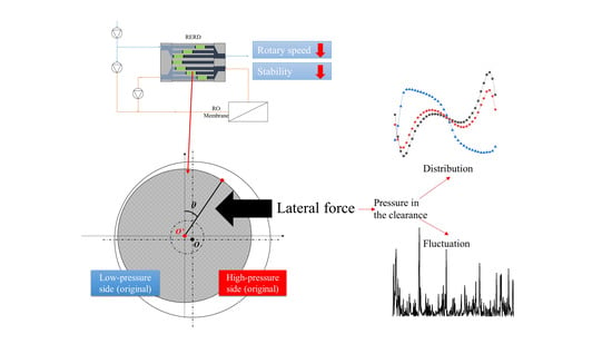
RERD in RO system(blue part is high-pressure and red part is low-pressure).
Water 16 00823 g001
Figure 2. Structure and working process of RERD. (a) Structure; (b) working process.
Water 16 00823 g002
Figure 3. Clearance between rotor and sleeve and the liquid film filling it.
Water 16 00823 g003
Figure 4. Axis section view of rotor and clearance and diagram of lateral force direction.
Water 16 00823 g004
Figure 5. Flow domain model of RERD and distribution of the sampling points. (a) End covers and rotor channels; (b) model with clearance and sampling points; (c) 3 sampling point circumferences; (d) number of circumferential sampling points.
Water 16 00823 g005
Figure 6. Mesh model (clearance part is not shown in the left side).
Water 16 00823 g006
Figure 7. Lateral force magnitude within one rotating cycle.
Water 16 00823 g007
Figure 8. Rotor channel position diagram corresponding to two pairs of peak and valley values of lateral force (the pink parts are rotor channels).
Water 16 00823 g008
Figure 9. Power spectral density curve of lateral force.
Water 16 00823 g009
Figure 10. Lateral forces in each direction and corresponding points’ pressure transient change curve. (a) Transient curve of lateral force in X direction and pressure of points at two sides of Y-axis; (b) transient curve of lateral force in X direction and pressure of points at two sides of Y-axis.
Water 16 00823 g010
Figure 11. Circular direction pressure distribution curve at circumference N-1, N-2, N-3 (red lines are fitting curves). (a) N-1; (b) N-2; (c) N-3.
Water 16 00823 g011
Figure 12. PSDM of pressure fluctuation and pressure standard deviation at each sampling point.
Water 16 00823 g012
Figure 13. PSDM at each sampling point.
Water 16 00823 g013
Figure 14. Diagram of rotor eccentricity.
Water 16 00823 g014
Figure 15. Diagram of the clearance pressure at the eccentric stable position.
Water 16 00823 g015
Figure 16. Pressure distribution curve in circular direction at eccentric stable position.
Water 16 00823 g016
Figure 17. Diagram of the range of pressure fluctuation with 32 times and 8 times rotation frequency.
Water 16 00823 g017
Figure 18. PSDM of each sampling point in the eccentric state.
Water 16 00823 g018
Figure 19. Pressure distribution curves of circumference N-1 under different flow rates and PHO. (a) Under different flow rates; (b) under different PHO.
Water 16 00823 g019
Figure 20. Change in lateral force under different working conditions (Red lines are fitting curves). (a) Under different flow rates; (b) under different PHO.
Water 16 00823 g020
Figure 21. Pressure distribution curves of the circumferences at the rotary speed of eccentric stabilization with different flow rates. (a) N-1; (b) N-2; (c) N-3.
Water 16 00823 g021
Figure 22. Circular pressure distribution curves at the rotary speed of eccentric stabilization with different PHO. (a) N-1; (b) N-2; (c) N-3.
Water 16 00823 g022
Figure 23. PSDM of the lateral force and excitation force under different working conditions. (a) Different flow rate; (b) different PHO.
Water 16 00823 g023
Figure 24. Fitted surface among the eccentric distance, flow rate and PHO.
Water 16 00823 g024
Figure 25. Fitted surface among the resistance torque, rotary speed and eccentric distance.
Water 16 00823 g025
Figure 26. Fitted surface of the rotary speed, flow rate and PHO on eccentric stabilization.
Water 16 00823 g026
Figure 27. Structure of four-districts RERD.
Water 16 00823 g027
Figure 28. Circumference pressure distribution fitting curves of four-districts RERD.
Water 16 00823 g028
Figure 29. Photos of test site and RERD components. (a) Experimental site; (b) parts of RERD.
Water 16 00823 g029
Figure 30. Sensors for rotary speed, pressure and vibration acceleration. (a) Rotary speed sensor; (b) pressure and vibration sensor.
Water 16 00823 g030
Figure 31. Time domain diagram of pressure fluctuation at point 34-1 in a rotation cycle (①–⑧ are 8 small cycle of fluctuation).
Water 16 00823 g031
Figure 32. PSD diagram of pressure fluctuation in frequency domain at point 34-1 in a rotation cycle.
Water 16 00823 g032
Figure 33. Comparison between simulation and experimental data of pressure mean value at point 34-1. (a) Different PHO; (b) different flow rate.
Water 16 00823 g033
Figure 34. Relation between the mean pressure at point 34-1 and PHO and flow rate in the experiment. (a) Different PHO; (b) different flow rate.
Water 16 00823 g034
Figure 35. Relation between the vibration RMS of the cylinder wall at point 34-1 and PHO and flow rate in the experiment. (a) Different PHO; (b) different flow rate.
Water 16 00823 g035
Figure 36. Rotary speed of rotor: comparison between the old model, new model and experimental data. (a) Different PHO; (b) different flow rate.
Water 16 00823 g036
Figure 37. Relation between the rotary speed of rotor and flow rate and PHO in the experiment. (a) Different PHO; (b) different flow rate.
Water 16 00823 g037
Table 1. Directions and characteristics of past research on RERD.
Research DirectionHighlightsWhat Can Be Improved
Static pressure supportThe lubrication, support and leakage mechanism of channel liquid film were revealed.The pressure distribution and lateral force was not researched.
Driving and resistance torqueThe hydraulic self-driving performance of RERD and rotary speed model were found.The eccentricity of the rotor was ignored.
Mixing behaviorThe mixing model was established and the mixing problem was improved a lot.Lack of comprehensive prediction formula of mixing rate.
Innovative structural designThe new structures exhibited higher energy recovery efficiency or lower energy cost.Few improvements were made to the stability of existing devices.
Table 2. Mesh number independence check.
Mesh Number (×106)Resultant Lateral Force (kN)Resistance Torque (N·m)
2.60138.38−3.680
3.07137.70−3.681
4.07138.67−3.676
Table 3. Change in the standard deviation of the mean values of pressure on each point on the circumference.
CircumferenceNon-EccentricEccentric
N-11.47 MPa1.49 MPa
N-2 1.69 MPa1.02 MPa
Table 4. Rotary speed and eccentric distance of the rotor under eccentric stabilization with different flow rates.
PHO (MPa)Flow Rate (m3/h)Rotary Speed (rpm)Eccentric Distance (μm)
69092011
68076012.5
67065013.5
66052014.5
65038016.5
Table 5. Rotary speed and eccentric distance of the rotor on eccentric stabilization under different PHO.
Flow Rate (m3/h)PHO (MPa)Rotary Speed (rpm)Eccentric Distance (μm)
70665013.5
705.567512.5
70568012
704.568511.3
70468810.5
703.56929.5
7036948.5
702.56967
7026985.5
701.56994.5
7017003
Table 6. Comparison between four-districts and the old two-districts RERDs.
Type of RERDLateral Force at Initial PositionExcitation Force at Stable Position
Old (two-districts)139 KN3.05 KN
Four-districts<2 kN1.70 KN
Disclaimer/Publisher’s Note: The statements, opinions and data contained in all publications are solely those of the individual author(s) and contributor(s) and not of MDPI and/or the editor(s). MDPI and/or the editor(s) disclaim responsibility for any injury to people or property resulting from any ideas, methods, instructions or products referred to in the content.

