
A Hybrid Coupled Model for Groundwater-Level Simulation and Prediction: A Case Study of Yancheng City in Eastern China

1
Key Laboratory of Virtual Geographic Environment (Nanjing Normal University), Ministry of Education, Nanjing 210023, China
2
State Key Laboratory Cultivation Base of Geographical Environment Evolution (Jiangsu Province), Nanjing 210023, China
3
School of Geographic Information and Tourism, Chuzhou University, Chuzhou 239000, China
4
School of Environmental Science, Nanjing Xiaozhuang University, Nanjing 211171, China
*
Authors to whom correspondence should be addressed.
Water 2023, 15(6), 1085; https://doi.org/10.3390/w15061085
Submission received: 31 January 2023
/
Revised: 23 February 2023
/
Accepted: 9 March 2023
/
Published: 12 March 2023
(This article belongs to the Special Issue Geohazards Monitoring Assessment: Earth-Observation Techniques)
Abstract
:The over-exploitation of groundwater has led to a significant drop in groundwater levels, which may lead to a series of geological disasters and ecological environmental problems such as ground subsidence and ground cracks. Therefore, through studying the dynamic change characteristics of groundwater, we can grasp the dynamic changes in groundwater level over time and invert the hydrogeological parameters, which provides an important basis for the management of groundwater resources. In this study, the confined aquifer III groundwater between 2005 and 2014 in Yancheng City was selected as the research object, and the Back Propagation (BP) neural network, Spatial-temporal Auto Regressive and Moving Average (STARMA) model, and BP-STARMA model were used to predict the spatial and temporal evolution trends of groundwater. In order to compare the prediction effectiveness of the BP-STARMA model, the fitting and prediction accuracies of the three models were measured from the perspectives of time and space. The results of the Relative Squared Error (RSE), Normal Mean Squared Error (NMSE), Root-Mean-Squared Error (RMSE), and Mean Absolute Error (MAE) were used to assess the robustness of the BP-STARMA model. The results showed that the fitting of the RMSE of BP-STARMA model was reduced by 39.92%, 38.35%, 30.25%, 31.55%, and 13.57% compared with the STARMA model, and by 22.2%, 8.7%, 15.9%, 28.5%, and 4.42% compared with the BP neural network model, respectively. Collectively, this shows that the BP-STARMA model has a better spatiotemporal prediction of groundwater level than the STARMA and BP neural network models, is more applicable to spatially continuous time-discrete spatiotemporal sequences, and is more applicable to spatiotemporal sequences that respond to natural geographic phenomena.
1. Introduction
Water is an indispensable resource for human beings, of which groundwater is one of the most important freshwater resources in geological structures [1,2,3]. With the rapid development and increase in the urban population and economy in eastern coastal areas of China, the demand for water resources is also increasing, and the intensity of groundwater mining is also strengthening gradually. However, excessive exploitation of groundwater will not only lead to the decrease in groundwater level, but also lead to water pollution [4], land subsidence [5,6], seawater intrusion [7,8,9], and other environmental hazards. In the eastern coastal areas of China, groundwater extraction reached its peak in the early 1990s, resulting in the continuous decline in groundwater level in these areas and the continuous development of geological disasters such as land subsidence and ground cracks. According to official groundwater monitoring reports, by the end of 2014, the cumulative land subsidence of coastal areas of Jiangsu Province is more than 200 mm, and the area of funnel formation is nearly 14,000 km2. The largest settlement center is located at Dafeng Haifeng Farm in Yancheng City, and the cumulative land subsidence is more than 700 mm.
Compared with surface water systems, the internal mechanisms of groundwater systems are more complex. As the change in water quantity and the migration laws of groundwater cannot be directly observed, and the geological harm caused by groundwater over-extraction is slow, once accumulated to a certain extent, it will cause irreversible damage. Therefore, relying on the monitoring data of groundwater dynamics, timely and accurate prediction of the dynamic change process of groundwater level and analysis of the dynamic change characteristics of groundwater are of great significance for groundwater exploitation and effective and sustainable management of water resources [10,11,12,13].
According to a review of the literature, dynamic prediction of groundwater levels is usually performed using either deterministic or stochastic models [14,15,16,17,18,19]. Deterministic models are solved by numerical model equations for known data, but deterministic models often require high data requirements and high costs, and realistic data inaccuracies and limited hydrogeological parameters make classical numerical models more uncertain [20]. The uncertainty of classical numerical models is compounded by the reality of inaccurate data and limited hydrogeological parameters. At the same time, changes in groundwater level are nonlinear and affected by multiple factors, such as precipitation, geological conditions, surface recharge, and human activities, which makes the prediction of groundwater very complicated. Therefore, it is necessary to establish a model reflecting the dynamic change law of groundwater levels by combining statistical theories [21,22]. As a natural phenomenon, the variations in groundwater tables are spatially continuous [23,24,25,26]. Therefore, the prediction of groundwater level changes should take into account both spatial and temporal factors [27].
With the rapid development of artificial intelligence computing, data-driven methods such as the artificial neural network (ANN) [28], support vector regression (SVR) [29], wavelet transform model [30,31], and extreme learning machine (ELM) [32,33] have been widely used in groundwater level prediction, and also provide a new method for modeling spatiotemporal series to solve complex nonlinear problems. Daliakopoulos investigated the performance of different neural networks in groundwater prediction and determined the optimal neural network structure to simulate the decreasing trend of groundwater level and predict the groundwater level over the next 18 months [34]. Lallahem proposed an artificial-neural-network-based approach using minimum lag and the number of hidden nodes to simulate the effective parameters and data in the groundwater level to generate the best performing simulation model [35]. Taormina and Mohammadi trained artificial neural network (ANN) simulations based on limited groundwater data to simulate and predict groundwater levels [36,37]. On the basis of principal component analysis, Sun combined the phase space reconstructed by chaos theory with a Back Propagation (BP) neural network, established the BP neural network model based on chaos theory, and predicted the groundwater level of Heihu Spring in Jinan [38]. Raj used artificial neural networks to predict rainfall and groundwater table depth [39]. Crespo [40] used the spatiotemporal autoregressive and moving average (STARMA) model for the short-term prediction of compressed sequence images, and the results showed that the STARMA model has good short-term prediction capability. Stroud [41] proposed a state-space framework for non-stationary spatiotemporal data and used tropical rainfall to demonstrate that the state-space model can handle non-stationary spatial processes and spatiotemporal correlations. Building on these premises, the current study set out to investigate space–time prediction using BP and STARMA models. In various studies, the STARMA model has been applied to rainfall forecasting [42,43], ecological management [44], temperature forecasting [45,46], and groundwater forecasting [47,48].
The groundwater levels are affected by a variety of factors, such as precipitation, hydrological conditions, surface recharge, and human activities, so it is difficult to predict dynamic groundwater levels [49,50]. The groundwater level monitoring data are typical spatiotemporal series with discrete time and continuous space [51]. The spatial distribution of aquifers is often continuous, and the spatial structure of time series changes slowly with the evolution of the environment, which belongs to the non-stationary spatial series, so the difference method is not applicable. For such spatiotemporal sequences, some methods that have been used to simulate and model non-stationary spatiotemporal data include Bayesian models [52], state-space models [53], and Kalman filtering methods [54], but most of these models are only applicable to specific areas. Therefore, it is necessary to seek a more general and applicable spatiotemporal modeling method for the nature of spatiotemporal sequences. The STARMA model has good applicability to smooth spatial and temporal series that are discrete in both time and space, but in fact, most spatial and temporal series are non-smooth. Martin proposed to use the difference method to transform non-smooth series into smooth ones and then apply the STARMA model to model them, but the difference method can only deal with temporal non-smoothness but not spatial non-smoothness. The BP neural network model can provide solutions for the realization and training of multi-layer neural networks, and is good at solving nonlinear problems. In addition, the groundwater level is affected by many factors such as climate and human activities, and its change law is nonlinear. The BP neural network model can effectively predict the nonlinear groundwater level. However, the prediction of the groundwater table should consider not only the temporal distribution but also the spatial heterogeneity. The STARMA model belongs to spatiotemporal modeling, which can consider the distribution of groundwater level data in time and space, and better cater to the spatiotemporal variation trend of groundwater level. This study focuses on the spatiotemporal series analysis of groundwater monitoring data and the interaction between the three models. The BP neural network model and STARMA model are combined effectively to simulate and predict the dynamic groundwater level, which can effectively improve the prediction accuracy of groundwater level.
2. Study Area and Methods
2.1. Overview of the Study Area
The study area of this paper was Yancheng City, Jiangsu Province, located in the east-central part of Jiangsu Province, China, with geographical coordinates of 33°15′~34°12′ N and 119°34′~120°41′ E. The total land area is about 6177.11 km2. The geographical location is shown in Figure 1. The study area is densely networked with water and meanders, and belongs to the coastal water network plain landform type. The topography of the study area is flat, with a general trend of high elevation in the southeast and low elevation in the northwest. The topography of the area is flat and slopes slowly from southeast to northwest.
The study area has deposited about 200.0~1600.0 m thick loose deposits since the Cenozoic, constituting a set of large thick underground water-bearing systems. The confined aquifers in the study area are mainly stored in the voids of loose sedimentary rock layers, with the burial depth range of 7.0~300.0 m, as shown in the hydrogeological profile in Figure 2. The lithology of the aquifers is mostly powdered sand, fine sand, and medium-fine sand, with abundant and stable water content. According to its stratigraphic conditions and hydrogeological characteristics, the area contains five aquifer groups: shallow groundwater and confined aquifers I, II, and III. The pore phreatic water and the confined aquifer I mainly receive infiltration recharge from atmospheric precipitation, surface water, and agricultural irrigation water, and the discharge mainly occurs through evaporation and exploitation, with poor water quality and little use value. The main exploitation is of the confined aquifers II and III, whose burial depth is determined by the basement structure, with a general trend of deep in the southeast and shallow in the northwest. The depth range of confined aquifer III is −126.0~−276.0 m, and the thickness is 5.0~70.0 m. It has good water richness and good water quality, so it is suitable for use as the main mining layer. Therefore, this paper selected confined aquifer III as the research object for the prediction of dynamic changes in groundwater.
The raw water level data for this experiment were taken from the database of groundwater level monitoring values for the area under the jurisdiction of the Yancheng Water Resources Bureau from 2005 to 2014. There are 133 monitoring wells in the city where the study area is located, of which 73 monitoring wells are distributed in the study area and 27 are confined aquifer III monitoring wells. The water level change values are monitored twice a month for each aquifer monitoring well and recorded in the database. The data from the monitoring wells selected in this paper were the water level monitoring data of the confined aquifer III monitoring wells from 2005 to 2014.
2.2. Data Analysis and Modeling Process
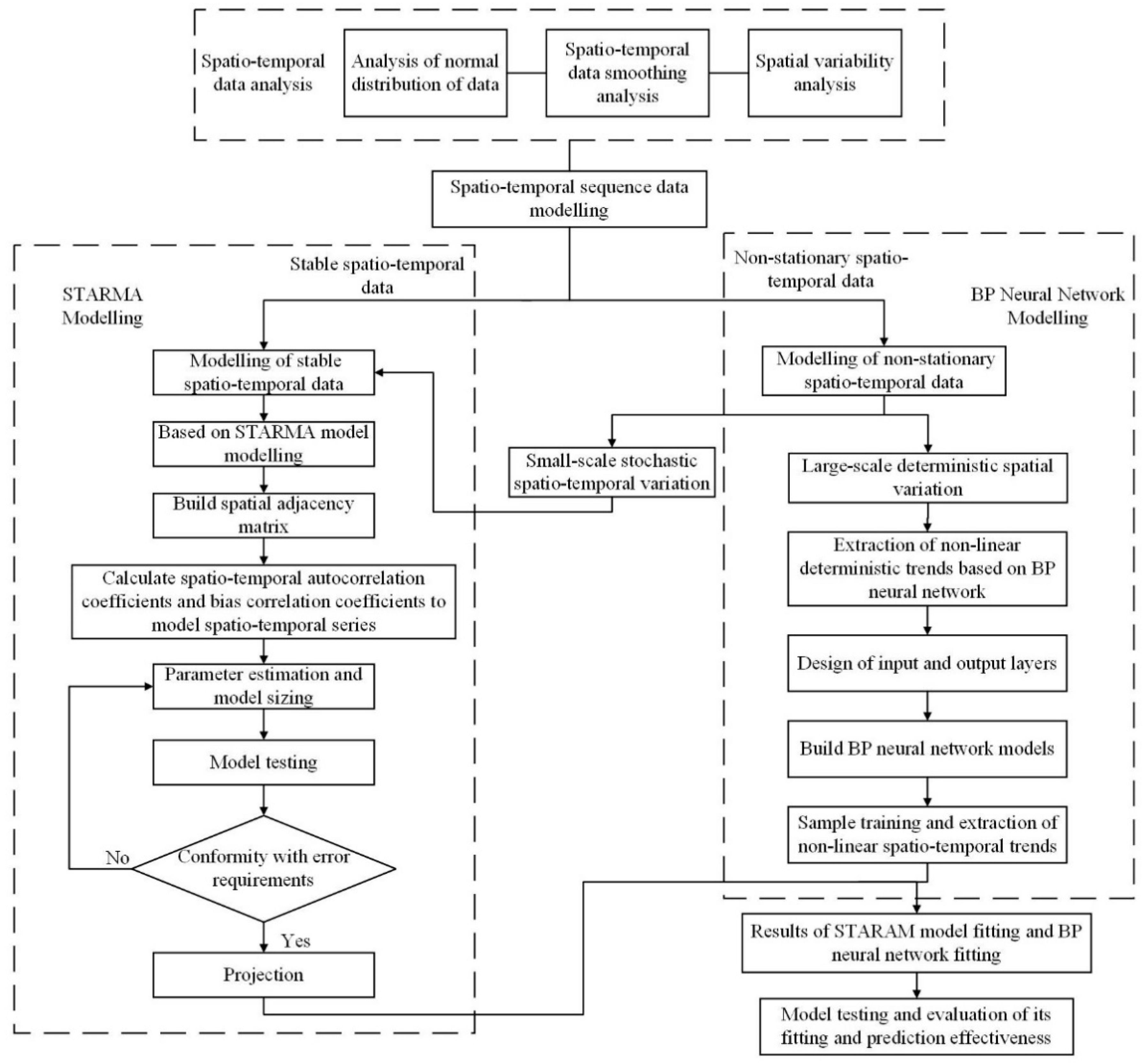
Figure 3 shows the construction process of the BP-STARMA model for the groundwater-level simulation, which consists of four parts, including the analysis of the spatiotemporal series of groundwater monitoring data, the establishment of the STARMA model, the establishment of the BP neural network model, and the establishment of the BP-STARMA model.
2.2.1. Spatiotemporal Data Analysis
Spatiotemporal sequence modeling is the modeling of spatiotemporal data by fitting properties to unobserved spatiotemporal locations. The modeling of spatiotemporal series data must take into account possible spatiotemporal dependencies in order to better represent spatiotemporal patterns and spatiotemporal relationships. Spatiotemporal autocorrelation is a measure of temporal and spatial correlation [56]. In this paper, the experimental data were analyzed and examined using exploratory spatiotemporal data analysis (ESTDA). ESTDA refers to the comprehensive application of the statistical method, exploratory spatial analysis method, and time series analysis method to test spatiotemporal data, which mainly include the following: the application of the calculation method to test the normal distribution of data; the spatial and temporal stationarity of data being tested by using spatial trend surface and time series graphs; the semi-variogram and Kriging interpolation being used to test the spatial correlation and spatial heterogeneity of the data.
- (1)
- Skewness coefficients, kurtosis coefficients, and non-parametric tests were used to determine whether the data were normally distributed. Analysis was performed using SPSS software(Version 21.0), and when the sample content n ≤ 2000, the results were based on the Shapiro–Wilk (W-test); when the sample content n > 2000, the results were based on the Kolmogorov–Smirnov (D-test). For unweighted or integer weights, the Shapiro–Wilk statistic was calculated when the weighted sample size was between 3 and 5000, while for single samples, the Kolmogorov–Smirnov test can be used to test whether the variables are normally distributed.
- (2)
- Time stationarity test [57]. This paper used the spatial trend analysis tool in ArcGIS to analyze the groundwater dynamic monitoring data in the study area as a trend surface to test the spatial smoothness; the test of temporal smoothness is mainly achieved through time series analysis. Time series analysis means that the time series is regarded as a random process that does not vary with time [58]. For a time series , the expression for the mean is
In Equation (1), the denotes the mean value of the spatiotemporal series; still denotes the spatial location i at the time t of observations; N denotes the number of spatial cells; T denotes the number of data periods.
- (3)
- Spatial variability analysis uses semi-variance functions to analyze spatial data. The semi-variance function , also known as the semi-variance function, is expressed as half of the variable between at points i and i + h and with the expression
In this paper, the kriging interpolation in ArcGIS was used to analyze the spatial variability of the object data.
2.2.2. STARMA Modeling
A spatiotemporal series analysis model involves the analysis, modeling and prediction of spatiotemporal series data, which can be viewed as a collection of spatially correlated time series [59,60,61,62]. The Spatiotemporal Auto Regressive and Moving Average (STARMA) model, which is essentially based on the Autoregressive and Moving Average (ARMA) model, considers the effect that spatial proximity has on it by using a time delay operator and a spatial delay operator to express how spatiotemporal variables are simultaneously affected by both time and space [56,63,64,65,66]. The STARMA model is more suitable for modeling geospatial and temporal sequence data as it fully takes into account the characteristics of geospatial and temporal autocorrelation [67].
According to the literature [68], STARMA modeling has three iterative steps: model identification, parameter estimation, and model testing.
- (1)
- The identification of the model is based on the truncated or trailing nature of its space–time autocorrelation function (STACF) and space–time partial autocorrelation function (STPACF). In this paper, based on the autocorrelation and bias correlation coefficients on the spatiotemporal data, the model chosen was identified as the spatiotemporal autocorrelation model STAR (2), with the specific expression
- (2)
- Estimation of the parameters in the model is carried out using the least-squares and greatest likelihood methods. That is, in order to make the model output value as close as possible to the actual monitoring value, the sum of squares of the error between the model output value and the actual monitoring value are used to measure, and the parameter value with the smallest sum of squares is the parameter value of the model.
- (3)
- Model validation. The residual sequence of the model is tested to determine whether it is a random error. If the residual of the model is random error—that is, the mean and auto-covariance of the model residual are 0, and the variance is σ2—then the model is reasonable; otherwise, the selected model is unreasonable, which means that there is a certain pattern in the residual sequence—that is, there is a certain correlation or variability in space–time. If the selected model is unreasonable, it means that there is still some important information in the original space–time sequence that has not been extracted, and then the model and parameter estimation need to be re-selected.
2.2.3. BP Neural Network Model Building
In this study, the MATLAB neural network toolbox was used to build the BP neural network topology. Spatiotemporal trends were extracted from the constructed BP neural network topology with the model functions of
In Equation (3), denotes the spatial location; n denotes the number of neurons in the hidden layer; denotes the trend value of the BP neural network at position i and time t; denotes the connection matrix weights of the hidden layer; denotes the threshold value; denotes the transfer function of the implicit layer; denotes the transfer function of the output layer.
In MATLAB, the premnmx function was used to normalize the input and output data of the network to between [−1, 1]; the Sigmoid transformation function was used to enable a BP network with an implicit layer to approximate any rational function with arbitrary accuracy; the Log-sigmoid function was used as the implicit layer transfer function and the purelin function as the output layer transfer function. Following this, the BP neural network was trained to fit the groundwater nonlinear variation trend values as a way to compare the effectiveness of the BP neural network fitting.
2.2.4. BP-STARMA Model Building
To address the spatial and temporal variability of the pore-bearing groundwater level monitoring data in nature, the BP neural network was first used to extract the spatial and temporal trend values of groundwater with its strong nonlinear fitting ability, and the sample residuals with the spatial and temporal trend values removed were fitted with the STARMA model.
As a typical spatiotemporal series, the dynamic monitoring sequence of the pore groundwater level can be described as:
In Equation (5), i denotes the spatial location of the spatiotemporal variables; t denotes the predicted time of the spatiotemporal variable; denotes the spatiotemporal variable in time t and spatial location i of the water level monitoring value; denotes the global deterministic spatiotemporal trend as a nonlinear variation function of ; denotes local stochastic spatiotemporal variability and is a spatiotemporal correlated error with a mean of zero.
In the BP-STARMA model, the BP neural network is first used to extract the trend of nonlinear dynamic changes in the spatiotemporal training dataset and then carry out the spatial correlation test for after removing the trend; if the spatial correlation condition is satisfied, then STARMA is applied to model the sample residuals after removing the spatiotemporal trend values; otherwise, the convergence accuracy of the neural network is appropriately reduced, and then the adjusted BP neural network is re-applied here to extract the trend values in the spatiotemporal series. In this paper, the BP network was used to extract the global deterministic spatiotemporal trend values in the spatiotemporal groundwater level series, and the STARMA model was applied to explain the residual series after the spatiotemporal trend values were removed; for the convenience of the latter, the above two models are jointly referred to as the BP-STARMA model.
3. Results and Discussion
3.1. Data Processing and Analysis
3.1.1. Monitoring Data Processing
The depth of the water level of confined aquifer III in the study area is higher in the east and lower in the west. The confined aquifer III in the eastern coastal area is buried at a depth of about 8.0 m. With the gradual extension of the aquifer to the west, the water level of confined aquifer III is also decreasing gradually. The buried depth of the groundwater level in the western region is mostly deeper than 20.0 m, and the buried depth of the groundwater level reaches about 32.0 m in Fuyang County and Yancheng urban area, which indicates that the groundwater in the study area has strong spatial heterogeneity. From the scope of the study area and the scope of a single monitoring well, the water level monitoring data of the confined aquifer III monitoring well from 2005 to 2014 in the study area were drawn, respectively, as the ‘water level–time’ variation curve, as shown in Figure 4, to analyze the dynamic variation characteristics of the groundwater level. In Figure 4, the average water level of each quarter in the horizontal coordinate is accumulated quarter by quarter since the first quarter of 2005. Figure 4a represents the change in the average lower water level of the whole study area over time, and Figure 4b represents the change in the water level of a single monitoring well over time. According to the analysis in Figure 4a, it can be seen that the groundwater level in the whole study area presents a downward trend. The blue in the Figure 4a represents the trend line of water level change; that is, there is a definite downward trend of water level in the entire study area. It can be seen from Figure 4b that the water level change curves of different water level monitoring wells show a certain randomness in different periods; that is, the water level change within the range of a single monitoring well shows a certain randomness. A comprehensive analysis shows that the characteristics of water level variation in the study area shows a certain decline trend in the global area and a certain random variation in the local area.
Groundwater level monitoring data of confined aquifer III in the study area were selected from the original database, and their spatial distribution is shown in Figure 1c. Most monitoring wells are distributed in the western part of the study area, while monitoring wells in the eastern coastal zone are less distributed. For individual monitoring wells with missing water level values in certain years, the ArcGIS spatial difference module or data statistics were used to obtain the results.
3.1.2. Data Analysis
Normal distribution test: This study used skewness and kurtosis coefficients and non-parametric methods to test the spatiotemporal data. The data from all monitoring wells were examined, and it was found that the monitoring wells numbered 51073006#, 51073509#, 51073512#, and 51074507# have a skewness or kurtosis greater than 1, as shown in Table 1, and their skewness u is greater than U0.05 = 1.96, which is tentatively considered not to conform to a normal distribution.
These four groups of data were re-run using SPSS for non-parametric tests, and the results are shown in Table 2. It was found that their P-test values (Sig2-tailed) are all less than 0.05; therefore, they do not conform to a normal distribution. In order not to affect the modeling accuracy, these 4 groups of monitoring data were removed from the dataset, and the remaining 23 monitoring wells’ monitoring data were selected as the experimental data.
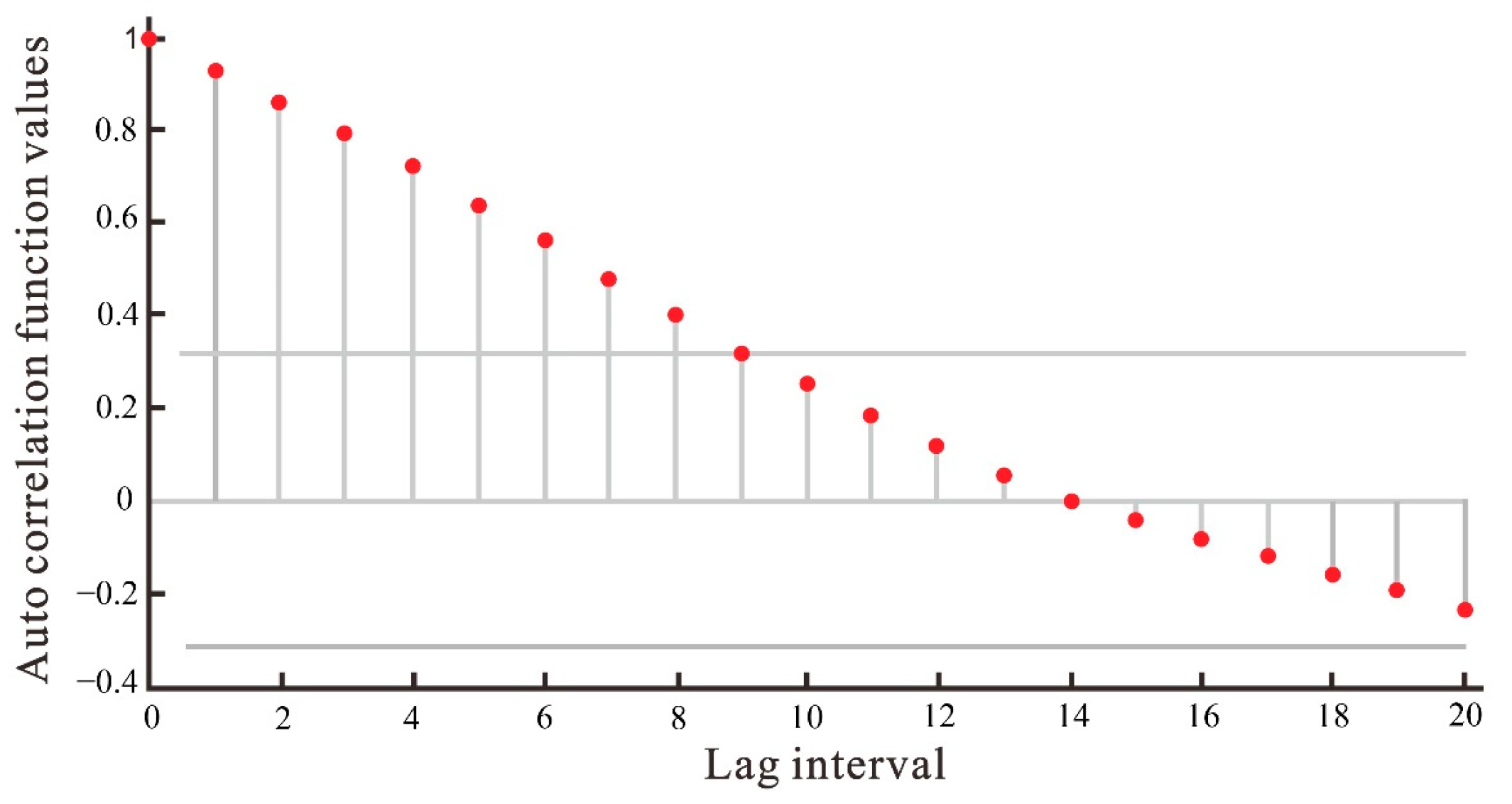
Test of time smoothness: The test of time smoothness is mainly achieved through time series analysis. The average groundwater level of confined aquifer III in the study area from 2005 to 2014 was calculated as shown in Table 3. In turn, a trend analysis of the time series water level monitoring data in Table 3 was made, as shown in Figure 4a, from which it can be seen that the average water level in the study area for 40 periods shows a decreasing trend. From Figure 5, it can be seen that the series only converges to zero after the delay interval of period 9 for the time autocorrelation function value (the area between the two grey bars in the graph), indicating that there is a degree of temporal correlation in the series and that the series is non-stationary in time.
Spatial variability analysis: The Kriging spatial interpolation method was used to obtain the elevation maps of the groundwater levels in the study area for the 10th, 20th, and 30th phases of the sample data and the 35th and 40th phases of the verification data. In the Figure 6b(elevation maps of the groundwater levels for 10th, 20th and 30th ), it can be seen that: first, there is a clear trend of decreasing water levels with the increase in years; secondly, there is a trend of decreasing minimum water level values year by year, while the maximum water level also decreases year by year; thirdly, the area of water levels in each class in the study area is also gradually increasing; fourthly, the water levels in the western part of the study area are clearly lower than those in the eastern part. The above combination indicates that the mean water levels in the study area have spatially heterogeneous characteristics for each period.
3.2. BP-STARMA Model Building
3.2.1. BP Neural Network to Extract Nonlinear Spatiotemporal Trends
After the spatiotemporal smoothness test described above, it was concluded that the spatiotemporal monitoring series of pore groundwater in the study area was a spatiotemporal non-smooth series and showed a decreasing trend throughout the study area, showing some randomness in the range of individual monitoring wells. Therefore, the BP neural network was used to extract the definite spatiotemporal trend values present in the groundwater of the study area.
In order to analyze the trend of groundwater level with seasonality, each quarterly data sample of water level monitoring was taken as one period and the data were the average of water level in each quarter; therefore, there were 40 periods (quarters) of data for each monitoring well in the study area for the 10 years from 2005 to 2014. In the BP neural network, the learning training data accounted for 70–80% of the total sample data and the validation data accounted for 20–30% of the total sample data, so the first 32 periods of all monitoring data of groundwater level in the study area were used as network learning training data and the last 8 periods were used as network validation data.
The trained BP neural network was used to fit the nonlinear trend value of the confined aquifer III in the study area, and the average groundwater level fitting value of the 10th, 20th, and 30th stages was obtained as shown in Figure 6. In the figure, green represents areas where water levels are deeply buried, while white represents areas where water levels are shallower.
3.2.2. STARMA Modeling
For the underground hydrogeological conditions in the study area, the spatial autocorrelation of the sample residuals used the semi-variance function (Equation (2)) to determine whether there was a spatial correlation distance between the sample residuals after removing the temporal trend values. The spatial variation in the study area was isotropic; that is, from west to east, and the semi-variance function analysis was carried out by selecting the appropriate number of periods of groundwater level values from the sample residuals to obtain the analysis results shown in Table 4. From the table, it can be seen that there is a spatial correlation distance in the residual series, which indicates that the sample residuals after removing the trend values are spatially correlated. In other words, the STARMA was used to model the residual series. The analysis results show that the residual series has relatively large bias abutment values and relatively small block gold values, indicating that the residual series has a strong spatial correlation.
The least-squares method was used to estimate the parameters of Formula 3 above, and the parameters and test values were obtained as shown in Table 5:
The prob in the table represents the significance levels of the t-statistic and are all less than 0.05, indicating that the coefficients are correlated with the dependent variable.
After the STARMA modeling of the residuals is completed, the residuals need to be tested. If the mean of the spatiotemporal autocorrelation coefficient values of the residuals is close to 0 and the variance is close to [N(T − S)]−1 (N = 23 indicates the number of spatial cells, T = 32 indicates the number of groundwater level monitoring periods, and s = 2 indicates the time delay), this indicates that the spatiotemporal autocorrelation function values are close to random errors. The values of the spatiotemporal autocorrelation coefficients calculated for the residuals of the model are shown in the Table 6 below.
As can be seen from the table, the spatially delayed autocorrelation coefficients of order 0 and order 1 are around 0, with mean values of 0.002 and −0.015, respectively, and variance values of 0.00112 and 0.00138, respectively, which are less than 1/[2332 − 2] = 0.00145, indicating that the model residuals are not significantly auto-correlated in time and space and the residual series are close to random errors, which explains how the STARMA model can better explain the spatiotemporal data of groundwater dynamic monitoring after removing the spatiotemporal trend values.
3.3. Comparison of Model Prediction Accuracy
According to Equation (5), the fitting result of the trend value extracted based on the BP neural network was added to the fitting value of the STARMA model to obtain the average fitting results of groundwater in the 10th, 20th, and 30th periods. The non-stationary spatiotemporal series was transformed into stationary series by Difference Methods (DMs), and the groundwater level was modeled by the STARMA model and BP neural network model. By comparing the three fitting results with the actual monitoring values, it can be seen that the BP-STARMA model can better fit the spatiotemporal evolution of groundwater. In order to further test the BP-STARMA, STARMA, and BP neural network models, the Root-Mean-Squared Error (RMSE) was used as an evaluation index to evaluate the fitting of the three models in different periods, and the evaluation results are shown in Table 7. The table shows that the standard deviation of fitting of BP-STARMA is smaller than those of the STARMA model and BP neural network model. Compared with the STARMA model and BP neural network model, the fitting accuracy of BP-STARMA is improved by 3.1% and 25.8%, and 19.5% and 7.5%, respectively.
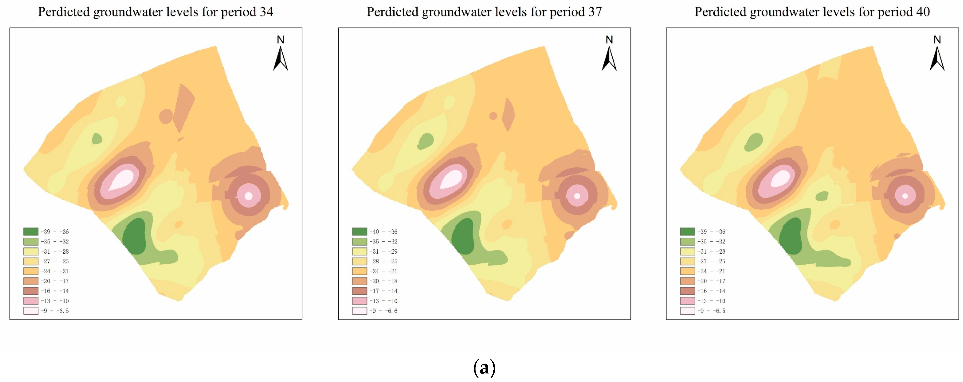
From the analysis of the BP-STARMA fitting effect, the model better fit the spatial and temporal variation pattern of groundwater in confined aquifer Ⅲ in the study area and the fitting result is better than the BP model and the STARMA model. However, the prediction results need to be verified to prove the good performance of the BP-STARMA model. Therefore, the above three models were used to validate the dynamic groundwater level monitoring data of the 33rd to 40th periods in the study area. Figure 7 shows the prediction results of the BP-STARMA model, STARMA model, and BP neural network model for the 34th, 37th, and 40th periods. At the same time, RMSE was also used to evaluate the fitting values of the three models at different periods, and the evaluation results are shown in the table.
The 34th BP-STARMA model, the STARMA model, and the BP neural network can all predict groundwater level values better, but as time increases, the STARMA model shows deviations between the predicted and actual monitored values, and the BP neural network model is less well fitted in local areas. The BP-STARMA model is better than the STARMA model and the BP network model in terms of prediction.
3.4. Evaluation and Comparison of Comprehensive Model Performance
In order to comprehensively compare the modeling effects of BP-STARMA, STARMA, and BP neural network models, we used four evaluation indexes to evaluate and compare the three models. They were the residual standard error (RSE), normalized mean squared error (NMSE), root-mean-squared error (RMSE), and mean absolute error (MAE). The values of the three models after evaluation are shown in Table 8.
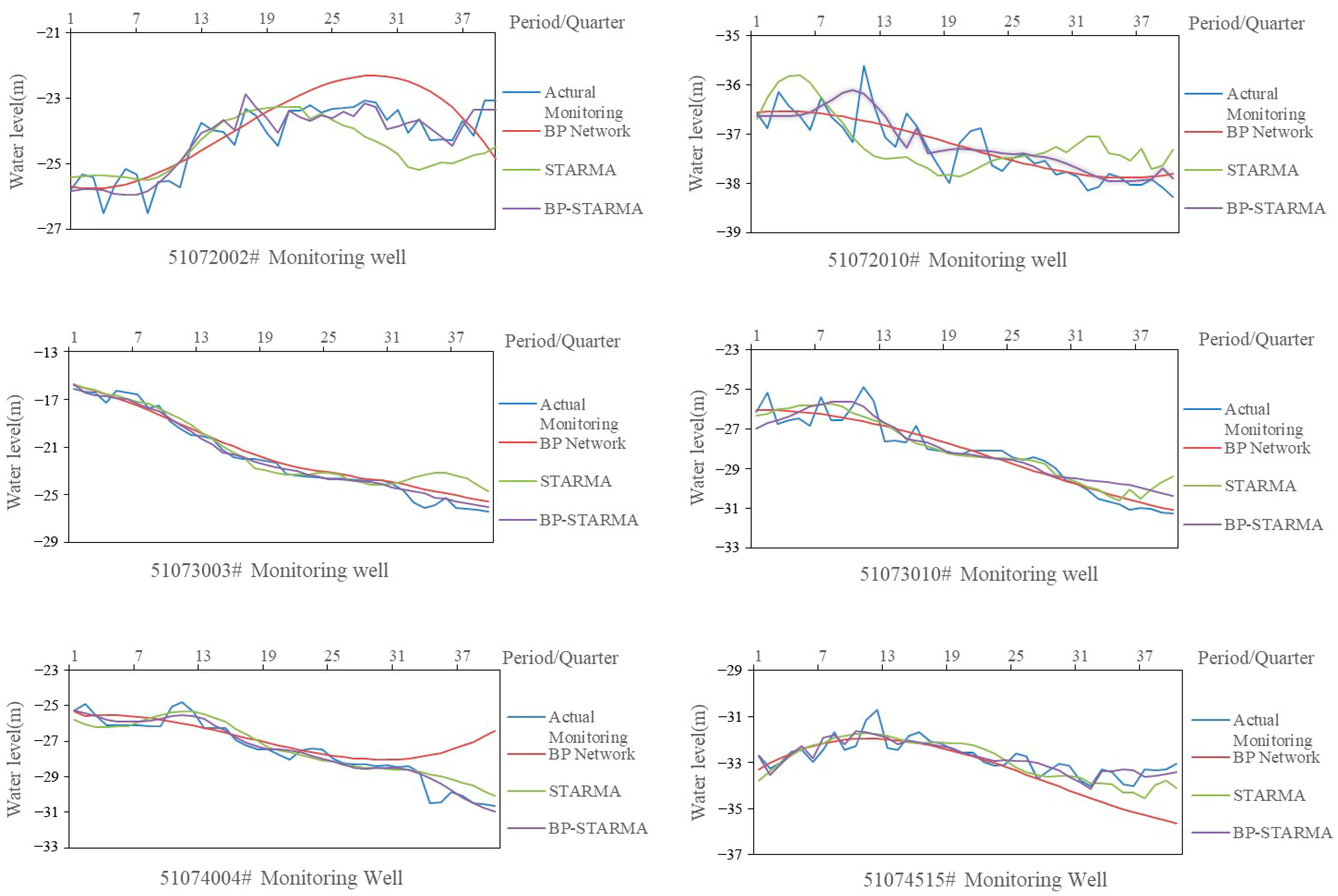
It can be seen from Table 9 that the evaluation indexes of BP-STARMA of the above six monitoring wells are lower than those of STARMA and BP, apart from the BP-STARMA evaluation indexes of the 51073010# monitoring well, which are higher than those of the STARMA model, which shows that the prediction effect of groundwater level based on the BP-STARMA model is better than that of the STARMA model and BP neural network model. That is, it has a good modeling effect for spatiotemporal data of continuous time discrete in space.
In order to more intuitively display the difference between the actual monitored values and the values of the three simulation models, we used a graph to describe the water level change curves of the above six monitoring wells, as shown in Figure 8.
In order to compare the fitting and prediction effects of the models separately, the fitting accuracy and prediction accuracy of BP-STARMA, STARMA, and BP neural network models were calculated separately using the RMSE evaluation index.Except for monitoring well 51073010#, the fitted root-mean-square error of the BP-STARMA model is reduced by 39.92%, 38.35%, 30.25%, 31.55%, and 13.57% compared to the STARMA model, and by 22.2%, 8.7%, 15.9%, 28.5%, and 4.42%, respectively, compared to the BP neural network model, indicating that the BP neural network has a better fit than STARMA. As for the prediction accuracy, the prediction accuracy of BP-STARMA is improved by 69.34%, 63.61%, 32.81%, and 47.28%, respectively, compared to the STARMA model, and 84.4%, 85.8%, 14.3%, 44.9%, 58.9%, and 55.4% compared to the BP neural network, which indicates that the STARMA model has a better prediction accuracy than the BP neural network model. It can be seen that the spatial and temporal fitting and prediction of groundwater level in the study area based on the BP-STARMA model are better than those of the STARMA model and the BP neural network model.
4. Conclusions
In this paper, three models, BP, STARMA, and BP-STARMA, were used to simulate and predict groundwater level changes for the spatiotemporal variation process of groundwater level. In the modeling using STARMA, the spatial variables tended to be isotropic in order to construct the spatial weight matrix, and the areas where the aquifers are continuous were selected; thus, the constructed models are suitable for areas with spatial continuity, but for phenomena where sharp extinction exists, a suitable model is not yet known. Based on the spatiotemporal variation characteristics of the groundwater level monitoring sequence, i.e., a global deterministic nonlinear variation trend value and a local stochastic spatial variation value, we constructed a BP neural network containing three input parameters to extract the global deterministic spatiotemporal trend value; a STARMA model was constructed for the residual values of the samples after removing the trend value, and finally, the BP model and the STARMA model were fitted to obtain the results. This showed that the BP-STARMA model was very effective in predicting the groundwater level in the study area. The results show that the BP-STARMA model is more applicable to the spatiotemporal series of continuous groundwater levels.
Author Contributions
Conceptualization, M.H. and S.C.; methodology, M.H. and L.H.; resources, S.C. and Z.H.; data analyses and software, M.H., X.C., and Z.H.; writing—original draft preparation, M.H. and X.C.; writing—review and editing, revising, L.H., M.H., and S.C. All authors have read and agreed to the published version of the manuscript.
Funding
This research was substantially supported by the Key Project of Natural Science Research in Universities of Jiangsu Province (No. 10KJA170028).
Data Availability Statement
The data presented in this study are available on request from the corresponding author. The data are not publicly available, due to privacy.
Conflicts of Interest
The data of this paper are original, and no part of this manuscript has been published or submitted for publication elsewhere. The authors declare no competing financial interest.
References
- Nourani, V.; Mousavi, S. Spatiotemporal groundwater level modeling using hybrid artificial intelligence-meshless method. J. Hydrol. 2016, 536, 10–25. [Google Scholar] [CrossRef]
- Sattari, M.T.; Mirabbasi, R.; Sushab, R.S.; Abraham, J. Prediction of Groundwater Level in Ardebil Plain Using Support Vector Regression and M5 Tree Model. Ground Water 2018, 56, 636–646. [Google Scholar] [CrossRef]
- Chen, W.; Li, H.; Hou, E.K.; Wang, S.; Wang, G.; Panahi, M.; Li, T.; Peng, T.; Guo, C.; Niu, C.; et al. GIS-based groundwater potential analysis using novel ensemble weights-of-evidence with logistic regression and functional tree models. Sci. Total Environ. 2018, 634, 853–867. [Google Scholar] [CrossRef] [Green Version]
- Yoon, H.; Kim, Y.; Lee, S.H.; Ha, K. Influence of the range of data on the performance of ANN- and SVM-based time series models for reproducing groundwater level observations. Acque Sotter. Ital. J. Groundw. 2019, 8, 17–21. [Google Scholar] [CrossRef]
- Rahmati, O.; Falah, F.; Naghibi, S.A.; Biggs, T.; Soltani, M.; Deo, R.C.; Cerdà, A.; Mohammadi, F.; Bui, D.T. Land subsidence modelling using tree-based machine learning algorithms. Sci. Total Environ. 2019, 672, 239–252. [Google Scholar] [CrossRef]
- Rahmati, O.; Golkarian, A.; Biggs, T.; Keesstra, S.; Mohammadi, F.; Daliakopoulos, I. Land subsidence hazard modeling: Machine learning to identify predictors and the role of human activities. J. Environ. Manag. 2019, 236, 466–480. [Google Scholar] [CrossRef] [PubMed]
- Conway, B.D. Land subsidence and earth fissures in south-central and southern Arizona, USA. Hydrogeol. J. 2016, 24, 649–655. [Google Scholar] [CrossRef]
- Gao, M.S.; Luo, Y.M. Change of groundwater resource and prevention and control of seawater intrusion in coastal zone. Bull. Chin. Acad. Sci. 2016, 31, 1197–1203. (In Chinese) [Google Scholar]
- Chen, S.M.; Liu, H.W.; Liu, F.T.; Miao, J.J.; Guo, X.; Zhang, Z.; Jiang, W.J. Using time series analysis to assess tidal effect on coastal groundwater level in Southern Laizhou Bay, China. J. Groundw. Sci. Eng. 2022, 10, 292–301. [Google Scholar]
- Mohanty, S.; Jha, M.K.; Kumar, A.; Sudheer, K.P. Artificial Neural Network Modeling for Groundwater Level Forecasting in a River Island of Eastern India. Water Resour. Manag. 2010, 24, 1845–1865. [Google Scholar] [CrossRef]
- Zou, J.; Xie, Z.; Zhan, C.; Qin, P.; Sun, Q.; Jia, B.; Xia, J. Effects of anthropogenic groundwater exploitation on land surface processes: A case study of the Haihe River Basin, northern China. J. Hydrol. 2015, 524, 625–641. [Google Scholar] [CrossRef]
- Abdollahi, S.; Pourghasemi, H.R.; Ghanbarian, G.A.; Safaeian, R. Prioritization of effective factors in the occurrence of land subsidence and its susceptibility mapping using an SVM model and their different kernel functions. Bull. Eng. Geol. Environ. 2019, 78, 4017–4034. [Google Scholar] [CrossRef]
- Natarajan, N.; Sudheer, C. Groundwater level forecasting using soft computing techniques. Neural Comput. Appl. 2020, 32, 7691–7708. [Google Scholar] [CrossRef]
- Liu, Y.J. The establishment and application of dynamic prediction model of groundwater level based on intelligent algorithm. Hydrogeol. Eng. Geol. 2004, 31, 55–56. [Google Scholar]
- Zhang, W.G.; Huang, Q.; Tong, C.S. Dynamic Prediction of Groundwater Level based on Chaos Optimization and Support Vector Machine. Resour. Sci. 2007, 29, 105–109. (In Chinese) [Google Scholar]
- Xu, J.; Chen, Y.; Li, W. Using GM (1,1) models to predict groundwater level in the lower reaches of Tarim River: A demonstration at Yingsu section. In Proceedings of the 2008 Fifth International Conference on Fuzzy Systems and Knowledge Discovery, Jinan, China, 18–20 October 2008; pp. 668–672. [Google Scholar]
- Fu, Z.; Liu, J.; Li, L.; Kong, M. Application of Artificial Neural Network in Dynamic Prediction of Groundwater Level in Weibei Irrigation Area. Bull. Soil Water Conserv. 2008, 4, 144–146. (In Chinese) [Google Scholar]
- Mohammad, R.; Ebadi, T.; Maknoun, R. Development of a smart model for groundwater level prediction based on aquifer dynamic condictions. Water Wastewater Winter 2011, 21, 70–80. [Google Scholar]
- Zhang, H.F. Overview on Groundwater Dynamic Prediction Model. Ground Water 2016, 1, 68–70. (In Chinese) [Google Scholar]
- Mohanty, S.; Jha, M.K.; Raul, S.K.; Panda, R.K.; Sudheer, K.P. Using Artificial Neural Network Approach for Simultaneous Forecasting of Weekly Groundwater Levels at Multiple Sites. Water Resour. Manag. 2015, 29, 5521–5532. [Google Scholar] [CrossRef]
- Lee, S.; Lee, K.K.; Yoon, H. Using artificial neural network models for groundwater level forecasting and assessment of the relative impacts of influencing factors. Hydrogeol. J. 2018, 27, 567–579. [Google Scholar] [CrossRef]
- Jeong, J.; Park, E. Comparative Applications of Data-Driven Models Representing Water Table Fluctuations. J. Hydrol. 2019, 572, 261–273. [Google Scholar] [CrossRef]
- Eriksson, E. Groundwater Time Series. Hydrol. Res. 1970, 1, 181–205. [Google Scholar] [CrossRef]
- Upton, K.A.; Jackson, C.R. Simulation of the spatio-temporal extent of groundwater flooding using statistical methods of hydrograph classification and lumped parameter models. Hydrol. Process. 2011, 25, 1949–1963. [Google Scholar] [CrossRef] [Green Version]
- Jha, M.K.; Sahoo, S. Efficacy of neural network and genetic algorithm techniques in simulating spatio-temporal fluctuations of groundwater. Hydrol. Process. 2015, 29, 671–691. [Google Scholar] [CrossRef]
- Ebrahimi, H.; Rajaee, T. Simulation of groundwater level variations using wavelet combined with neural network, linear regression and support vector machine. Glob. Planet. Chang. 2017, 148, 181–191. [Google Scholar] [CrossRef]
- Nourani, V.; Ejlali, R.G.; Alami, M.T.; Aalami, M.T. Spatiotemporal Groundwater Level Forecasting in Coastal Aquifers by Hybrid Artificial Neural Network-Geostatistics Model: A Case Study. Environ. Eng. Sci. 2011, 28, 217–228. [Google Scholar] [CrossRef]
- Rakhshandehroo, G.R.; Vaghefi, M.; Aghbolaghi, M.A. Forecasting groundwater level in Shiraz Plain Using Artificial Neural Networks. Arab. J. Sci. Eng. 2012, 37, 1187–1883. [Google Scholar] [CrossRef]
- Zhou, T.; Wang, F.; Yang, Z. Comparative analysis of ANN and SVM models combined with wavelet preprocess for groundwater depth prediction. Water 2017, 9, 781. [Google Scholar] [CrossRef] [Green Version]
- Behnia, N.; Rezaeian, F. Coupling wavelet transform with time series models to estimate groundwater level. Arab. J. Geosci. 2015, 8, 8441–8447. [Google Scholar] [CrossRef]
- Afkhamifar, S.; Sarraf, A. Comparative study of groundwater level forecasts using hybrid neural network models. Proc. Inst. Civ. Eng.-Water Manag. 2021, 174, 267–277. [Google Scholar] [CrossRef]
- Hussein, E.A.; Thron, C.; Ghaziasgar, M.; Bagula, A.; Vaccari, M. Groundwater prediction using machine-learning tools. Algorithms 2020, 13, 300. [Google Scholar] [CrossRef]
- Seidu, J.; Ewusi, A.; Kuma, J.S.Y.; Ziggah, Y.Y.; Voigt, H.J. A hybrid groundwater level prediction model using signal decomposition and optimized extreme learning maching. Model. Earth Syst. Environ. 2022, 8, 3607–3624. [Google Scholar] [CrossRef]
- Daliakopoulos, I.N.; Coulibaly, P.; Tsanis, I.K. Groundwater Level Forecasting Using Artificial Neural Networks. J. Hydrol. 2005, 309, 229–240. [Google Scholar] [CrossRef]
- Lallahem, S.; Mania, J.; Hani, A.; Najjar, Y. On the use of neural networks to evaluate groundwater levels in fractured media. J. Hydrol. 2005, 307, 92–111. [Google Scholar] [CrossRef]
- Mohammadi, K. Groundwater Table Estimation Using MODFLOW and Artificial Neural Networks. Pract. Hydroinformatics 2009, 68, 127–138. [Google Scholar]
- Taormina, R.; Chau, K.W.; Sethi, R. Artificial neural network simulation of hourly groundwater levels in a coastal aquifer system of the Venice lagoon. Eng. Appl. Artif. Intell. 2012, 25, 1670–1676. [Google Scholar] [CrossRef] [Green Version]
- Sun, X.L.; Xu, X.C.; Tan, Y.M. BP Neural Network Model Based on Chaos Theory and Application in Ground Water Level Forecasting. In Proceedings of the 2008 2th International Symposium on Intelligent Information Technology Application, Shanghai, China, 21-22 December 2008; pp. 445–448. [Google Scholar]
- Raj, A.S.; Oliver, D.H.; Srinivas, Y.; Viswanath, J. Wavelet based analysis on rainfall and water table depth forecasting using Neural Networks in Kanyakumari district, Tamil Nadu, India. Groundw. Sustain. Dev. 2017, 5, 178–186. [Google Scholar]
- Crespo, J.L.; Zorrilla, M.; Bernardos, P.; Mora, E. A new image prediction model based on spatio-temporal techniques. Vis. Comput. Int. J. Comput. Graph. 2007, 23, 419–431. [Google Scholar] [CrossRef]
- Stroud, J.R.; Müller, P.; Sansó, B. Dynamic models for spatiotemporal data. J. R. Stat. Soc. Ser. B (Stat. Methodol.) 2001, 63, 673. [Google Scholar] [CrossRef]
- Li, Z.H.; Miao, Z.H. A new precipitable water vapor STARMA model based on Newton’s method. Adv. Intell. Syst. Comput. 2016, 367, 275–287. [Google Scholar]
- Saha, A.; Singh, K.N.; Ray, M.; Rathod, S. A hybrid spatio-temporal modelling: An application to space-time rainfall forcasting. Theor. Appl. Climatol. 2020, 142, 1271–1282. [Google Scholar] [CrossRef]
- Rathod, S.; Saha, A.; Patil, R.; Ondrasek, G.; Gireesh, C.; Anantha, M.S.; Rao, D.V.K.N.; Bandumula, N.; Senguttuvel, P.; Swarnaraj, A.K.; et al. Two-stage spatiotemporal time series modelling approach for rice yield prediction & advanced agroecosystem management. Agronomy 2021, 11, 12. [Google Scholar]
- Saha, A.; Singh, K.N.; Ray, M.; Rathod, S.; Dhyani, M. Fuzzy rule-based weighted space-time autoregressive moving average models for temperature forecasting. Theor. Appl. Clim. 2022, 150, 1321–1335. [Google Scholar] [CrossRef]
- Kumar, R.R.; Sarkar, K.A.; Dhakre, D.S.; Bhattacharya, D. A hybrid space-time modelling approach for forecasting monthly temperature. Environ. Model. Assess. 2022, 1–14. [Google Scholar] [CrossRef]
- Ahmadi, R.; Shahrabi, J.; Aminshahidy, B. Forecasting multiple-well flow rates using a novel space-time modeling approach. J. Pet. Sci. Eng. 2020, 191, 107027. [Google Scholar] [CrossRef]
- He, L.; Hou, M.Q.; Chen, S.Z.; Zhang, J.; Chen, J.; Qi, H. Construction of a spatio-temporal coupling model for groundwater level prediction: A case study of Changwu area, Yangtze River Delta region of China. Water Supply 2021, 21, 3790–3809. [Google Scholar] [CrossRef]
- Sivajogi, D.; Koppula. Forecasting Groundwater Levels: A Stochastic Procedure. Transp. Res. Rec. 1984, 965, 16–21. [Google Scholar]
- Pourtaghi, Z.S.; Pourghasemi, H.R. GIS-based groundwater spring potential assessment and mapping in the Birjand Township, southern Khorasan Province, Iran. Hydrogeol. J. 2014, 22, 643–662. [Google Scholar] [CrossRef]
- Demel, S.S.; Du, J. Spatio-temporal models for some data sets in continuous space and discrete time. Stat. Sin. 2015, 25, 81–98. [Google Scholar]
- Mclaughlin, D.B. Hanford Groundwater Modeling: A Numerical Comparison of Bayesian and Fisher Parameter Estimation Techniques; Resource Management Associates: Lafayette, CA, USA, 1980. [Google Scholar]
- Hamilton, J.D. State-space models. Handb. Econom. 1986, 4, 39–50. [Google Scholar]
- Zadrozny, P.A.; Mittnik, S. Kalman-filtering methods for computing information matrices for time-invariant, periodic, and generally time-varying VARMA models and samples. Comput. Math. Appl. 1994, 28, 107–119. [Google Scholar] [CrossRef] [Green Version]
- He, L.; Chen, L.; Chen, S.Z. Visualization method for porous groundwater seepage flow field based on particle flow: Case of Yancheng city in the East coast of China. Geofluids 2022, 2022, 4850968. [Google Scholar] [CrossRef]
- Martin, R.L.; Oeppen, J.E. The Identification of Regional Forecasting Models Using Space: Time Correlation Functions. Trans. Inst. Br. Geogr. 1975, 66, 95–118. [Google Scholar] [CrossRef]
- George, E.P.B.; Gwilym, M.J.; Gregory, C.R.; Greta, M.L. Time Series Analysis; Wiley: Hoboken, NJ, USA, 2008; pp. 47–91. [Google Scholar]
- Cao, Q.; Yue, D.; Gao, Y.; Wang, X. Contrast Study on Various Methods Extracting Trend Extraction Based on Non-stationary Time Series. J. Geod.Geody. (In Chinese). 2013, 33, 150–154. [Google Scholar]
- Wang, G.; Yang, P.; Daren, L. Method of Spatio-Temporal Series and Tests Analysis on Its Predictable Skill. Chin. J. Atmos. Sci. 2004, 28, 536–544. [Google Scholar]
- Patle, G.T.; Singh, D.K.; Sarangi, A.; Rai, A.; Khanna, M.; Sahoo, R.N. Time Series Analysis of Groundwater Levels and Projection of Future Trend. J. Geol. Soc. India 2015, 85, 232–242. [Google Scholar] [CrossRef]
- Barzegar, R.; Fijani, E.; Moghaddam, A.A.; Tziritis, E. Forecasting of Groundwater Level Fluctuations Using Ensemble Hybrid Multi-wavelet Neural Network-based Models. Sci. Total. Environ. 2017, 599, 20–31. [Google Scholar] [CrossRef] [PubMed]
- Al-Haija, Q.A. A machine learning based predictive model for time-series modelling and analysis. Int. J. Spatio-Temporal Data Sci. 2021, 1, 270–283. [Google Scholar] [CrossRef]
- Cliff, A.D.; Ord, J.K. Space-Time Modelling with an Application to Regional Forecasting. Trans. Inst. Br. Geogr. 1975, 64, 119–128. [Google Scholar] [CrossRef]
- Pfeifer, P.E.; Deutsch, S.J. Identification and Interpretation of First Order Space-Time ARMA Models. Technometrics 1980, 22, 397–408. [Google Scholar] [CrossRef]
- Pfeifer, P.E.; Deutsch, S.J. Independence and sphericity tests for the residuals of space-time arma models Independence and sphericity tests for the residuals. Commun. Stat.—Simul. Comput. 1980, 9, 533–549. [Google Scholar] [CrossRef]
- Tao, C.; Jiaqiu, W.; Xia, L. A Hybrid Framework for Space-Time Modeling of Environmental Data. Geogr. Anal. 2011, 43, 188–210. [Google Scholar]
- Zhou, M.; Buongriorno, J. Space-Time Modeling of Timber Prices. West. J. Agric. Econ. 2006, 31, 40–56. [Google Scholar]
- Pfeifer, P.E.; Deutsch, S.J. STARIMA (Space-Time Autoregressive Integrated Moving Average) Model-Building Procedure with Application to Description and Regional Forecasting; Bureau of Justice Statistics: Washington, DC, USA, 1979.
Figure 1.
Geographical location map of the study area. (a) Jiangsu Province, China; (b) Yancheng City; (c) spatial location of boreholes in the study area.
Figure 1.
Geographical location map of the study area. (a) Jiangsu Province, China; (b) Yancheng City; (c) spatial location of boreholes in the study area.

Figure 2.
Hydrogeological profile of the study area [55].
Figure 2.
Hydrogeological profile of the study area [55].

Figure 3.
Flow chart of groundwater level prediction based on the coupled BP-STARMA model.

Figure 4.
(a) Diagram of the average water level variation of confined aquifer III; (b) diagram of water level variation of different monitoring wells of confined aquifer III.
Figure 4.
(a) Diagram of the average water level variation of confined aquifer III; (b) diagram of water level variation of different monitoring wells of confined aquifer III.

Figure 5.
Autocorrelation function of mean groundwater table. Red dots represent the time autocorrelation function value of the groundwater level.
Figure 5.
Autocorrelation function of mean groundwater table. Red dots represent the time autocorrelation function value of the groundwater level.

Figure 6.
(a) Spatiotemporal trend map extracted by BP neural network; (b) Average groundwater level of the 10th, 20th, and 30th periods.
Figure 6.
(a) Spatiotemporal trend map extracted by BP neural network; (b) Average groundwater level of the 10th, 20th, and 30th periods.

Figure 7.
Comparison of predicted values and actual verification data of different models in different monitoring periods. (a) Groundwater level elevation map fitted by BP-STARMA model; (b) groundwater level elevation map fitted by STARMA model; (c) groundwater level elevation map fitted by BP neural network model; (d) groundwater level elevation map fitted by actual monitoring values.


Figure 8.
Groundwater fitting and predicted change curves for different models at different monitoring wells.
Figure 8.
Groundwater fitting and predicted change curves for different models at different monitoring wells.


Table 1.
Results of skewness and kurtosis coefficient tests.
| Monitoring Well Number | Bias u | Peak State u |
|---|---|---|
| 51073006# | 3.075023 | 0.559089 |
| 51073509# | 3.136233 | 0.852506 |
| 51073512# | 2.765471 | 1.891852 |
| 51074507# | 2.712559 | 0.273745 |
Table 2.
Results of the non-parametric test.
| 51073006# | 51073509# | 51073512# | 51074507# | ||
|---|---|---|---|---|---|
| N | 40 | 40 | 40 | 40 | |
| Normal | Mean | −30.8653 | −19.5038 | −7.69125 | −36.1275 |
| Parameters a,b | Std. Deviation | 2.783878 | 2.366837 | 0.55931 | 3.325536 |
| Most Extreme Differences | Absolute | 0.320592 | 0.195934 | 0.159134 | 0.166015 |
| Positive | 0.320592 | 0.195934 | 0.159134 | 0.166015 | |
| Negative | −0.17658 | −0.10716 | −0.08156 | −0.15888 | |
| Test Statistic | 0.320592 | 0.195934 | 0.159134 | 0.166015 | |
| Asymp. Sig. (2-tailed) | 0.000 c | 0.000 c | 0.012 c | 0.007 c | |
Notes: a. Test distribution is normal. b. Calculated from data. c. Lilliefors significance correction.
Table 3.
Average water level data for the study area.
| Number of Issues | Water Level (m) | Number of Issues | Water Level (m) | Number of Issues | Water Level (m) | Number of Issues | Water Level (m) |
|---|---|---|---|---|---|---|---|
| 1 | −22.322 | 11 | −23.344 | 21 | −25.103 | 31 | −25.977 |
| 2 | −22.161 | 12 | −23.540 | 22 | −25.182 | 32 | −26.212 |
| 3 | −22.323 | 13 | −24.108 | 23 | −25.285 | 33 | −26.154 |
| 4 | −22.492 | 14 | −24.138 | 24 | −25.327 | 34 | −25.336 |
| 5 | −22.468 | 15 | −24.268 | 25 | −25.345 | 35 | −26.486 |
| 6 | −22.726 | 16 | −24.574 | 26 | −25.461 | 36 | −26.536 |
| 7 | −22.556 | 17 | −24.646 | 27 | −25.751 | 37 | −26.553 |
| 8 | −22.879 | 18 | −24.744 | 28 | −25.810 | 38 | −26.621 |
| 9 | −22.833 | 19 | −24.971 | 29 | −25.698 | 39 | −26.703 |
| 10 | −22.338 | 20 | −25.090 | 30 | −25.810 | 40 | −26.844 |
Table 4.
Residual semi-variance analysis results.
| Number of Issues | Variable Range (km) | Offset Abutment Value (C) | Nugget Value (C0) | Abutment Values (C0 + C) | C0/Sill (%) |
|---|---|---|---|---|---|
| 4 | 21.7 | 18.42 | 4.99 | 23.41 | 21.32 |
| 8 | 20.7 | 16.24 | 5.21 | 21.45 | 24.29 |
| 12 | 22.8 | 15.32 | 7.73 | 23.05 | 33.54 |
| 16 | 21.4 | 16.42 | 10.83 | 27.25 | 39.74 |
| 20 | 21.8 | 14.77 | 10.88 | 25.65 | 42.42 |
| 24 | 21.3 | 18.63 | 9.94 | 28.57 | 34.79 |
| 28 | 21.5 | 13.19 | 12.71 | 25.9 | 49.07 |
Table 5.
STARMA model parameter estimation results.
| Coefficient | Std. | t-Statistic | Prob | |
|---|---|---|---|---|
| 0.54276 | 0.06895 | 4.5148 | 0.0132 | |
| 0.15267 | 0.07429 | 6.8419 | 0.0051 | |
| −0.38156 | 0.06472 | 6.7513 | 0.0024 | |
| 0.24158 | 0.05719 | 3.4856 | 0.0084 |
Table 6.
Spatial and temporal autocorrelation coefficients of sample residuals.
| Space Delay (h) Time Delay (k) | 0 | 1 | Space Delay (h) Time Delay (k) | 0 | 1 |
|---|---|---|---|---|---|
| 1 | 0.038 | −0.073 | 9 | 0.064 | −0.042 |
| 2 | −0.012 | −0.028 | 10 | 0.013 | 0.026 |
| 3 | 0.048 | −0.035 | 11 | −0.016 | −0.092 |
| 4 | −0.04 | −0.023 | 12 | 0.068 | −0.0011 |
| 5 | −0.03 | 0.017 | 13 | −0.0093 | 0.0017 |
| 6 | −0.027 | −0.021 | 14 | −0.037 | 0.061 |
| 7 | −0.034 | 0.019 | 15 | 0.0061 | −0.0347 |
| 8 | 0.017 | −0.068 | 16 | −0.015 | 0.0015 |
Table 7.
RMSE values of three different models in different monitoring periods.
| Periods | Fitted Values | Periods | Predicted Values | ||||
|---|---|---|---|---|---|---|---|
| RMSE | RMSE | ||||||
| BP-STARMA | STARMA | BP | BP-STARMA | STARMA | BP | ||
| 10 | 0.662993 | 0.684267 | 0.630171 | 34 | 1.104 | 1.25 | 1.34 |
| 20 | 0.397683 | 0.536424 | 0.493816 | 37 | 1.38 | 1.1642 | 1.91 |
| 30 | 0.369923 | 0.361022 | 0.399997 | 40 | 2.20 | 2.718 | 2.69 |
Table 8.
Comprehensive evaluation results of different models.
| Indicators | Models | 51072002# | 51072010# | 51073003# | 51073010# | 51074004# | 51074515# |
|---|---|---|---|---|---|---|---|
| RSE | BP-STARMA | 0.150101 | 0.283151 | 0.016342 | 0.220120 | 0.053888 | 0.303071 |
| STARMA | 0.604417 | 0.904445 | 0.114733 | 0.049426 | 0.117395 | 0.53618 | |
| BP | 0.828549 | 0.427072 | 0.022214 | 0.449457 | 0.399316 | 0.394206 | |
| NMSE | BP-STARMA | 0.000254 | 0.000119 | 0.000381 | 0.000630 | 0.000205 | 0.000128 |
| STARMA | 0.001012 | 0.000278 | 0.001797 | 0.000105 | 0.000448 | 0.000226 | |
| BP | 0.00199 | 0.000247 | 0.000525 | 0.001161 | 0.000851 | 0.000239 | |
| RMSE | BP-STARMA | 0.385879 | 0.347153 | 0.425131 | 0.704296 | 0.393573 | 0.370956 |
| STARMA | 0.774334 | 0.620444 | 1.126466 | 0.333735 | 0.580906 | 0.493408 | |
| BP | 1.0878 | 0.587649 | 0.500338 | 0.957361 | 0.798729 | 0.507498 | |
| MAE | BP-STARMA | 0.315065 | 0.263823 | 0.339018 | 0.58108 | 0.27274 | 0.291155 |
| STARMA | 0.619108 | 0.493683 | 0.767228 | 0.244518 | 0.44759 | 0.408922 | |
| BP | 0.6692 | 0.449455 | 0.388958 | 0.627958 | 0.56586 | 0.377935 |
Table 9.
RMSE values of three different models in different monitoring periods.
| Monitoring Well Number | Fitted Values | Predicted Values | ||||
|---|---|---|---|---|---|---|
| RMSE | RMSE | |||||
| BP-STARMA | STARMA | BP | BP-STARMA | STARMA | BP | |
| 51072002# | 0.3955 | 0.6583 | 0.5089 | 0.3448 | 1.1245 | 2.2092 |
| 51072010# | 0.3814 | 0.6187 | 0.4180 | 0.1440 | 0.3957 | 1.0137 |
| 51073003# | 0.3177 | 0.4555 | 0.3779 | 0.7070 | 2.3483 | 0.8249 |
| 51073010# | 0.5780 | 0.2346 | 0.4510 | 1.0695 | 0.5803 | 1.9414 |
| 51074004# | 0.2968 | 0.4336 | 0.4152 | 0.6497 | 0.9670 | 1.5812 |
| 51074515# | 0.3648 | 0.4221 | 0.3817 | 0.3745 | 0.7104 | 0.8396 |
Disclaimer/Publisher’s Note: The statements, opinions and data contained in all publications are solely those of the individual author(s) and contributor(s) and not of MDPI and/or the editor(s). MDPI and/or the editor(s) disclaim responsibility for any injury to people or property resulting from any ideas, methods, instructions or products referred to in the content. |
© 2023 by the authors. Licensee MDPI, Basel, Switzerland. This article is an open access article distributed under the terms and conditions of the Creative Commons Attribution (CC BY) license (https://creativecommons.org/licenses/by/4.0/).
Share and Cite
MDPI and ACS Style
Hou, M.; Chen, S.; Chen, X.; He, L.; He, Z. A Hybrid Coupled Model for Groundwater-Level Simulation and Prediction: A Case Study of Yancheng City in Eastern China. Water 2023, 15, 1085. https://doi.org/10.3390/w15061085
AMA Style
Hou M, Chen S, Chen X, He L, He Z. A Hybrid Coupled Model for Groundwater-Level Simulation and Prediction: A Case Study of Yancheng City in Eastern China. Water. 2023; 15(6):1085. https://doi.org/10.3390/w15061085
Chicago/Turabian StyleHou, Manqing, Suozhong Chen, Xinru Chen, Liang He, and Zhichao He. 2023. "A Hybrid Coupled Model for Groundwater-Level Simulation and Prediction: A Case Study of Yancheng City in Eastern China" Water 15, no. 6: 1085. https://doi.org/10.3390/w15061085
Note that from the first issue of 2016, this journal uses article numbers instead of page numbers. See further details here.