Germany-Wide High-Resolution Water Balance Modelling to Characterise Runoff Components as Input Pathways for the Analysis of Nutrient Fluxes

Abstract

The input of nutrients into surface waters and groundwater is directly linked to runoff components. Due to the different physicochemical behaviour of nitrogen and phosphorus compounds, the individual runoff components have different significance as input pathways. Within the scope of the Germany-wide project AGRUM-DE, spatially differentiated runoff components were modelled with the water balance model mGROWA at a resolution of 100 m. The modelled distributed runoff components include total runoff, surface runoff, drainage runoff, natural interflow, direct runoff from urban areas, and groundwater recharge. Although the mGROWA model operates in daily time steps, modelled runoff components can be aggregated to mean long-term hydrologic reference periods—for this study, 1981–2010. We obtained good model agreement through the comparison of measured discharge from 298 river gauges against the spatial means of the modelled runoff components over their corresponding catchment areas. Therefore, the model results provide reliable input for input pathway-specific modelling of actual nutrient inputs as well as scenario analyses expected from the application of nutrient reduction initiatives. This ensures that any differences in the model results stem exclusively from differences in nutrient supply (fertilisation of the soils) and not from climatic effects, such as the influence of wet or dry years.

1. Introduction and Objective

The input of nutrients into surface waters and groundwater is directly linked to runoff components [1]. The simulation of the runoff components at a high spatial resolution is, therefore, a prerequisite for the accurate modelling of nitrogen (N) and phosphorous (P) inputs into receiving waters, differentiated according to the discharge pathways [2,3,4].

Total runoff in a catchment corresponds to the difference between the amount of precipitation and the amount of actual evapotranspiration. Total runoff can be separated into its runoff components (Figure 1), which discharge into the receiving waters either via the unsaturated zone or via aquifers [5,6]. Surface runoff is the portion of runoff that flows on the land surface into receiving water without having infiltrated into the soil [7]. A second runoff component that falls into this category is direct runoff from urban areas, i.e., runoff from sealed areas that is collected by urban systems without having infiltrated into the soil [8]. After a precipitation event, both surface runoff and runoff from urban systems generally reach the receiving water in a timeframe of several minutes to more than an hour [9,10].

Water infiltrating into the soil is referred to as percolation water or leachate [11]. Leachate either percolates through the entire unsaturated zone and infiltrates into the aquifer or accumulates in the unsaturated zone above a layer of low hydraulic conductivity. In the latter case, water in the unsaturated zone moves laterally downslope towards receiving water without reaching the aquifer. This runoff component is referred to as natural interflow [12,13]. Natural interflow is especially significant in humid, mountainous bedrock regions. The flow time of natural interflow is usually in the order of one to several days before it reaches a receiving water body [14].

In lowland areas of humid climate regions, water discharge from the root zone of groundwater-affected or waterlogged soils has often been accelerated through the installation of drainage systems such as pipe (tile) and trench (open ditch) drainage systems [15]. From a hydrological perspective, drainage systems represent rapid runoff pathways that are comparable in their effect on natural interflow.

All runoff components that reach a receiving water body only with a short time delay after a runoff-triggering precipitation event, i.e., drainage runoff, natural interflow, surface runoff, and direct runoff from settlement areas, are considered direct runoff according to German standards [16].

Groundwater recharge refers to the portion of the percolation water that actually infiltrates into an aquifer, thus replenishing groundwater resources [17]. Over periods of several years to decades, the quantity of groundwater recharge can often be considered to be equivalent to the exfiltration from the aquifer into the receiving water [18]. This exfiltration can be considered as the baseflow [19], which is often used for the validation of modelled groundwater recharge [20,21]. This is because during longer dry periods only the baseflow is measured at the gauges. In a catchment, this mean long-term baseflow generally corresponds to the mean long-term groundwater discharge to a surface water body. The latter corresponds to the mean long-term groundwater recharge in the catchment area concerned. Therefore, the baseflow can be considered a good proxy for the validation of modelled mean long-term groundwater recharge in a catchment [19].

Whereas point-source N and P discharges to surface waters via separate and combined sewer systems typically stem from urban direct runoff, diffuse N and P inputs to surface waters can be traced back to the runoff components (i.e., input pathways). As the physicochemical behaviour of N and P compounds vary from each other, the individual runoff components have different levels of importance as input pathways.

A fraction of the nitrate input into the soil is retained by microbiological net immobilisation in soils [22,23] or degraded by denitrification processes in soils [24,25,26]. Another part (fertilisation, atmospheric deposition) is taken up by plants. The residual nitrate is highly soluble in water and does not bind to soil particles. Thus, diffuse nitrate inputs into soils are translocated in dissolved form via runoff components. This occurs: (i) via natural interflow and drainage runoff, where nitrate reaches a receiving water body with only a short time lag after a runoff-triggering precipitation event [27,28]; and (ii) via groundwater-borne runoff, where nitrate reaches a receiving water body after a long time lag [29], under the condition that full denitrification does not first occur in the aquifer [30].

Unlike nitrate compounds, P compounds typically do not undergo degradation in either soils or groundwater. Instead, P can be adsorptively bound to soil particles. The most important diffuse input pathway for P in many regions is, therefore, water erosion [31], through which P bound to soil particles (particulate P) reaches receiving waters via surface runoff. Particulate P and to an extent dissolved P enter drainage systems in the soil and the connected receiving waters via macropores [32]. While particulate P inputs into surface waters via groundwater discharge can largely be excluded, dissolved P inputs into surface waters via groundwater discharge do occur. Some of these inputs are considered to be of anthropogenic origin [33]. As diffuse P input to surface waters occurs via groundwater-borne discharge, the modelled groundwater recharge is also important for simulating diffuse P input to surface waters.

A key requirement for modelling N and P inputs to receiving waters by input pathways is, therefore, the simulation of runoff components and nutrient displacement at high spatial resolution. Physically based hydrological models for this purpose, such as WaSIM-ETH [34] and MIKE SHE/MIKE 11 [35], are based on the physics of hydrological processes and are suitable for simulations at a regional scale, e.g., for individual mesoscale catchments [36,37,38]. Physically based reactive N and P transport models [39,40,41] belong to the same model type. In general, they have been coupled with physically based hydrologic models to simulate N and P displacement and retention in soils at a high temporal and spatial resolution. The application of such models on larger scales is possible, provided that suitable input data are available [42] and that computational time requirements are not a limiting factor [43].

Models used for nutrient management at the national scale are typically less complex and require less input data and less computational time [44]. For this purpose, integrated modelling approaches are usually used that combine coupled hydrological or nutrient transport models with agro-economic models [45]. Typical applications of such models are the determination of current N and P loads to groundwater and surface waters [46,47] and the prediction of the efficacy of nutrient reduction measures [48,49].

In Europe, the application of integrated nutrient flux models at the country level is often related to the requirements arising from the implementation of the EU Nitrate Directive [50], the EC Water Framework Directive [51], and the EU Marine Strategy Framework Directive [52]. In Germany, the AGRUM-DE-model network was developed as an integrated nationwide model to quantify N and P inputs into groundwater and surface waters [53,54]. The AGRUM-DE-model network consists of the regionalised agricultural and environmental information system (RAUMIS) of the Thünen Institute in Braunschweig [45,55], the hydrological/hydrogeological model system mGROWA-DENUZ-WEKU-MEPhos of Forschungszentrum Jülich [24,47,56,57], and the nutrient input model MONERIS of the Leibniz Institute for Freshwater Ecology and Inland Fisheries in Berlin [58,59,60].

This contribution focuses on the mGROWA model, which is a key component of the AGRUM-DE model for the German-wide identification of runoff components and nutrient input pathways. The article comprises:

• An introduction to the daily-scale water balance model mGROWA with a focus on the modules for the determination of input pathways for the assessment of nutrient fluxes;
• Germany-wide results for the individual runoff components as long-term mean averages for the time period 1981–2010 and elaboration of the corresponding regionally dominant input pathways;
• A statistical evaluation of mGROWA model results with respect to observed runoff records to assess the representativeness of the modelled nutrient input pathways;
• A discussion of the mGROWA modelling within the context of the overarching goals in the AGRUM-DE project.

2. Determination of Runoff Components

Within the Germany-wide AGRUM-DE project, we implemented the mGROWA model [61], which is a deterministic, distributed (grid-based) water balance model (Figure 2). The mGROWA model was selected for two reasons: (i) because of both the ability to model at the extremely high spatial resolution required to adequately capture heterogeneous site conditions while maintaining a feasible computation time; and (ii) due to the ability to disaggregate the complex multiple flow components that are relevant for nutrient modelling.

We defined the spatial resolution of the model grid based on the resolution of the available input data whilst ensuring that the computational time for the model was not excessive. In the context of the nationwide mGROWA application in Germany, a 100 m grid was chosen. The model has approximately 35.7 million individual grid cells, for which the runoff components were then simulated individually. For the model setup, we implemented seven soil layers, each 30 cm deep.

In the mGROWA model, actual evapotranspiration and total runoff are first calculated in daily time steps. Actual evapotranspiration is calculated based on potential evapotranspiration over grass [63,64], land use-specific k_c coefficients [65], a topographic correction function [66], and the Disse equation to account for the dependence of evapotranspiration on soil moisture [67]. To calculate soil moisture and percolation water dynamics for sites covered with vegetation, mGROWA contains the multilayer soil–water balance model BOWAB [68]. Depending on the water tension in the root zone, a capillary rise is calculated for sites with near-surface groundwater, meaning that at these sites, evapotranspiration from groundwater can occur. Additionally, mGROWA calculates the evaporation from impervious areas [57]. More details about the determination of actual evapotranspiration and runoff using the mGROWA model can be found in the corresponding literature [57,61,69,70].

Separation of the total runoff into the direct runoff components (surface runoff, direct runoff from urban areas, natural interflow, drainage runoff) and groundwater recharge follows a hierarchical approach (Figure 3), based on identified site conditions (Figure 2).

For each individual grid cell, the model checks whether there is any surface sealing. In this case, over the portion of the grid cell that has sealing, the generated runoff is subdivided into direct runoff from urban surfaces, i.e., the portion of runoff that is discharged via rainwater sewers, and the portion that infiltrates into the soil. Not all impervious areas have a connection to a sewer system; for example, runoff may seep away elsewhere, and not all surfaces are hydraulically dense enough so that no seepage water movement can take place beneath them. To consider this, a surface sealing percolation index (SSPI) splits the runoff generated over sealed surfaces into urban direct runoff and a subsurface runoff portion, depending on the degree of imperviousness. This subsurface runoff component, together with the runoff formed over the previous portion of a grid cell, is separated into groundwater recharge and other subsurface direct runoff components [69].

Over unsealed surfaces, surface runoff is the transport medium of nutrient inputs into surface waters via wash-off and erosion. However, only areas that have a hydraulic connection to surface water contribute to N and P inputs via these input pathways. Further site conditions include a slope greater than 2%, high clay content in the topsoil, agricultural use, and no artificial drainage [31,71,72]. Only when all of these conditions are met, the grid cell is identified as a “delivery area” for N and P inputs via surface runoff. For all other grid cells, all surface runoff is assumed to infiltrate into the soil after a short flow distance at the surface, meaning that potentially washed-off and eroded N and P loads do not reach receiving water. Therefore, the surface runoff is modelled exclusively for the grid cells that are connected to a recipient and that have relevance for nutrient input. For these specified grid cells, the method for quantifying mean long-term surface runoff varies according to hydrogeological conditions. For most areas, surface runoff is calculated based on mean long-term precipitation and gross total runoff [73], while for areas with unconsolidated rock, no near-surface groundwater, and no soil waterlogging (Figure 3), surface runoff is calculated using total runoff and slope.

As a next step, the presence of near-surface groundwater is checked. If no near-surface groundwater exists, a differentiation is made between unconsolidated rock and bedrock. For bedrock, baseflow indices (BFI) [74,75,76,77] are applied to quantify the separation of the groundwater recharge from natural interflow. The premise behind this concept is that over a long period, the groundwater recharge as a fraction of the total runoff can be regarded as constant over areas with comparable hydrogeological site characteristics. The BFI concept assumes that long-term groundwater discharge and groundwater recharge of a catchment are equal, provided that the total groundwater resources of the area remain unchanged. The BFIs can theoretically assume values between 0 and 1. A value of 0 means that an aquifer cannot store any infiltrating water, while a value of 1 means that the entire leachate infiltrates into the aquifer. BFI values have been determined for numerous site characteristics, predominantly according to aquifer typologies and/or hydraulic conductivities [66,74,78,79,80,81,82].

For grid cells with near-surface groundwater, the runoff separation follows a different concept. Initially, the model checks whether artificial drainage of agricultural land is expected. In this case, in unconsolidated rock areas, the installation depth of agricultural drainage systems [83] and the seasonally fluctuating groundwater tables in soil directly control the separation of the leachate into drainage runoff and groundwater recharge [82]. Drainage runoff is generated exclusively in the period when the groundwater table has risen above the installation depth of the drainage systems.

For grid cells showing near-surface groundwater and no artificial drainage, percolation water reaches the groundwater surface directly and, thus, becomes groundwater recharge by definition. Due to capillary rise from groundwater, depletion of groundwater resources can occur at these sites, especially in the summer months. To account for these interactions, mGROWA calculates the net groundwater recharge, which assumes negative values in the months in which capillary rise dominates.

For unconsolidated rocks without near-surface groundwater, the soil waterlogging characteristics and the topographical slope are considered. When waterlogging in the soil is associated with agricultural land use, it is assumed that drainage systems have been installed [84]. For such sites, BFI values are used that divide the total runoff into fixed portions of drainage runoff and groundwater recharge depending on the waterlogging class of the soil and land use. For other land uses, it is assumed that drainage systems have not been installed. In this case, waterlogging in the soil causes the generation of natural interflow. For grid cells that have neither groundwater influence nor waterlogging in the soil but do have a substantial slope, slope-dependent BFI values are implemented, separating the total runoff into groundwater recharge and either natural interflow for grid cells without connection to receiving surface waters or surface runoff for grid cells with water connection. For grid cells with neither waterlogging nor a substantial slope, the entire leachate is modelled as groundwater recharge.

3. Input Data

A prerequisite for the modelling is a digital geographic reference map of Germany for which the model grid is defined and to which all input datasets and model calculations are related to. For this purpose, the UTM 32N with ellipsoid GRS80 and datum ETRS89 was used. Based on the geometries of this digital map, all vector-based input data of the mGROWA model have been converted into raster data.

Some loss of information will always occur when transforming vector data into the raster format required for modelling. A study of conversions of vector soil map data to model grids of varying spatial resolutions demonstrated that model grids of 50 m or 100 m are sufficient to ensure adequate representativeness in the raster grid [85].

For hydrological modelling over large areas, grid-cell sizes of less than 100 m only marginally reduce the information loss of maps, but exponentially increase the computational effort [85]. Therefore, a 100 m grid was considered optimal for the Germany-wide model determination of runoff components and diffuse nutrient inputs in the AGRUM-DE project.

The mGROWA modelling in the AGRUM-DE-project was performed using nationwide datasets (

Table 1. Model input data.

Data Type	Data Source
Land use	Federal Agency for Cartography and Geodesy - Digital Land Cover Model for Germany (LBM-DE2015)
Imperviousness	Copernicus Land Monitoring Service - High-Resolution Layer Imperviousness (2012) 20 m
Digital elevation model	Federal Agency for Cartography and Geodesy (BKG) - Digital Terrain Model grid width 25 m (DGM25)
Soil map and database - Soil horizon parameters (thickness of horizons, (effective) field capacity, soil texture, bulk density, substance volume) - Soil profile parameters (waterlogging, groundwater influence)	Federal Institute for Geology and Natural Resources (BGR) - Soil map BUEK200 v0.6 1:200,000
Drained areas	Forschungszentrum Jülich, IBG-3
Climate data (1981–2010) - Precipitation - Potential evapotranspiration	Climate Data Center (CDC) of the German Weather Service (DWD)
Hydrogeological parameters - Baseflow index	Forschungszentrum Jülich, IBG-3
Discharge data	German Federal Institute of Hydrology (BfG) - Database with daily discharge measurements
Gauges as point coordinates with associated catchment sizes	German Hydrological Yearbook (DGJ)
Catchment areas of gauges	Forschungszentrum Jülich, IBG-3

) provided by water management authorities and the statistical offices of the federal and state governments. Only datasets that are available nationwide were considered.

Of the input datasets listed in Table 1, only precipitation data are visualised since this is the key input variable from which discharge and all runoff components relevant for nutrient export are derived.

Monthly precipitation sums are derived from raster files of 1 × 1 km spatial resolution, disaggregated to the 100 × 100 m model raster. The long-term mean annual precipitation for the modelling period of 1981–2010 is shown here (Figure 4, left).

Additionally, daily precipitation sums from station data are derived to specify the temporal distribution within each simulated month. Figure 4 (right) shows the spatial distribution of 4987 rain gauge stations with data available over the modelling period.

The weather-exposed ridges of the low mountain ranges (e.g., Harz Mountains, Black Forest, Rhenish Slate Mountains, Bavarian Forest) and the Alps strongly influence the distribution of precipitation in Germany. The Luv effect, i.e., the lifting of air masses due to the morphological conditions, is evident in these regions. As a result of the maritime winds predominantly from southwest to northwest, precipitation quantities of more than 1000 mm/a occur in these regions. In the Alps, this precipitation can increase to more than 2000 mm/a with a transition to the Alpine foothills, where precipitation between 1500 mm/a and 2000 mm/a occurs.

From west to east, precipitation decreases significantly and is below 600 mm/a in many parts of the northeast. In the western states, low precipitation occurs only in lowland areas located in the rain shadow of the low mountain ranges, such as the northern part of the Upper Rhine Valley, the southern part of the Lower Rhine Valley, and Franconia. In the other parts of the country, mean annual precipitation levels are relatively uniform between 600 and 850 mm/a, with a north–south gradient evident. With increasing distance from the North Sea and the Baltic Sea, precipitation decreases.

4. Modelled Runoff Components (Nutrient Input Pathways)

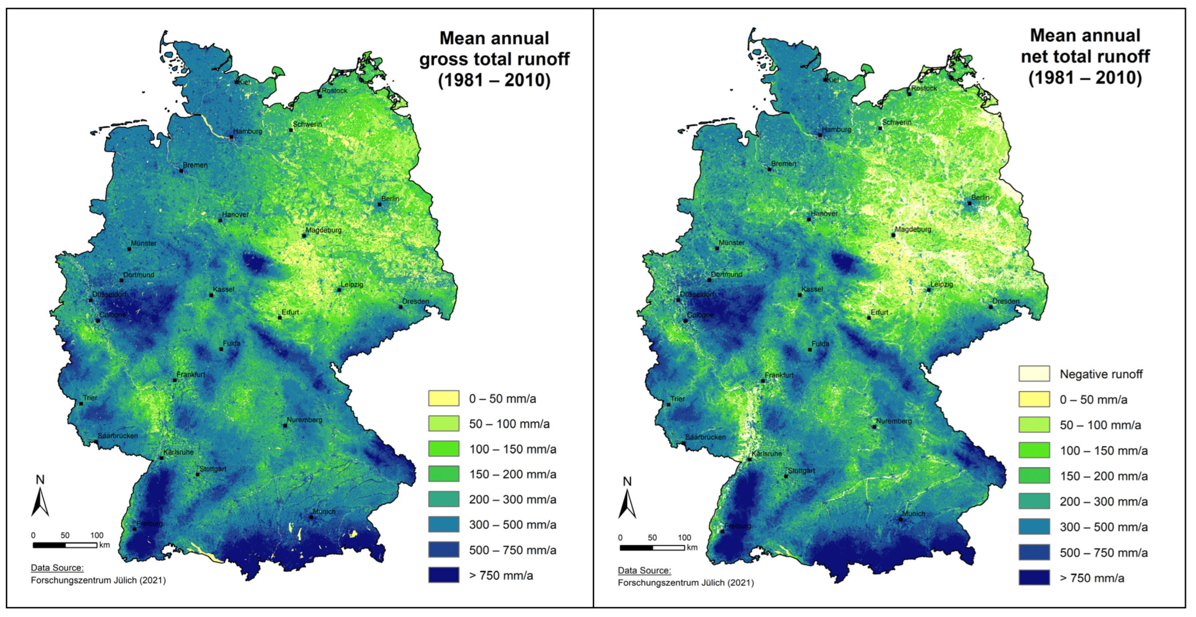
4.1. Total Runoff

The total runoff refers to the difference between precipitation and the actual evapotranspiration from the earth’s surface based on the general hydrological water balance equation.

There are two ways in which total runoff can be defined: net total runoff or gross total runoff. Net runoff represents the runoff generation minus capillary rise and direct evapotranspiration from groundwater, while gross runoff represents generation on a grid cell without consideration of capillary rise or direct evapotranspiration from groundwater. In grid cells that have near-surface groundwater, evapotranspiration is increased by a capillary rise from groundwater into the root zone of soils to such an extent that actual evapotranspiration may exceed the total runoff. This situation is most common in lowland regions where for some grid cells, long-term means show negative total runoff. The associated total runoff represents the net total runoff, which is suitable for comparison with measured mean long-term discharge values at gauges.

Because gross total runoff does not consider capillary rise or direct evapotranspiration from groundwater, the values for individual grid cells cannot be negative. Despite being possible that no total runoff is generated in years with low precipitation because all precipitation is “consumed” for the evapotranspiration process, gross total runoff over a long period of time is always positive. This means that runoff is generated and nutrients can be displaced. Therefore, gross total runoff is more suitable than net total runoff as a starting point for dividing total runoff into the individual runoff components and the determination of the input pathways for nutrients to surface waters and groundwater. Note that gross total runoff and net total runoff are identical in regions without capillary rise of groundwater.

Figure 5 (left) shows the spatial distribution of the mean annual gross total runoff for 1981–2010 and Figure 5 (right) shows the net total runoff. Gross total runoff of more than 500 mm/a occurs mainly in the high altitudes of the low mountain ranges (Rhenish Slate Mountains, Harz, Thuringian Forest, Black Forest, Bavarian Forest) and in the Alps. In the other low mountain regions (e.g., Palatinate Forest, Weser Uplands, South German stratified plain) as well as in the western part of the North German lowlands, the total runoff ranges between approximately 200 mm/a and 500 mm/a.

In some larger river valleys in the low mountain range (Danube, Main, Nahe, Lahn), as well as in the southern part of the Lower Rhine Embayment, the total runoff values range between 100 and 200 mm/a. In general, low precipitation of often less than 800 mm/a and high potential evapotranspiration have a limiting effect on the total runoff. Due to precipitation of less than 600 mm/a, total runoff of less than 100 mm/a occurs in the northeast and some parts of southwest Germany,

Net total runoff considers capillary rise and direct evapotranspiration from groundwater so it differs from gross total runoff in areas with near-surface groundwater and drainage systems. Negative runoff can be observed in lowland regions where evapotranspiration exceeds the total runoff in large parts of northeast Germany, e.g., Elbe Valley, but also in parts of southwest Germany, e.g., the Upper Rhine Valley.

4.2. Surface Runoff and Urban Direct Runoff

The surface runoff and urban direct runoff are the two runoff components that do not infiltrate into the ground before reaching surface water.

The surface runoff is generally low compared with other runoff components (Figure 6, left). Depending on the precipitation level, however, surface runoff of more than 50 mm/a can occur over non-forested areas in the low mountain ranges. In the Alps and Alpine foothills, surface runoff of more than 300 mm/a is sometimes simulated. In contrast, for large forest areas such as the ridges of the Bavarian Forest and the Black Forest, no significant surface runoff is modelled, despite high precipitation and a hydraulic connection to surface water. In areas with less than 800 mm annual precipitation and shallow slopes, surface runoff is negligible. This site condition applies to most of the North German lowlands but also to parts of the Rhine Valley plains. Accordingly, N and P inputs via wash-off and erosion can be excluded as main input pathways in such regions.

Figure 6 (right) shows the mean annual urban direct runoff for the fraction of runoff generation in urban areas that originates from sealed surfaces. This is used to calculate N and P inputs from point sources to surface waters via separate and combined sewer systems. Direct runoff from urban areas can exceed 300 mm/a in the central areas of larger settlements such as Berlin, the Ruhr area, and Hamburg.

4.3. Discharge via Natural Interflow and via Drainage Systems

The predominant direct runoff component in bedrock regions is natural interflow (Figure 7, left). With mean long-term natural runoff of more than 750 mm/a, the Alps and the Paleozoic bedrock regions (Rhenish Slate mountains, Harz mountains, Black Forest) stand out clearly. Substantially lower natural interflow (<300 mm/a) occurs in the area of the Mesozoic rock sequences, e.g., in the South German stratified plain and in the Weser Uplands, due to the high proportion of groundwater recharge designated by the corresponding BFI values.

In the parts of Germany situated in the lees of the low mountain ranges (e.g., Rhenish Hesse, Upper Rhine Valley, Lower Rhine Embayment, Thuringian Basin), as well as in regions where karstified carbonate rocks are present, the mean long-term natural interflow rarely exceeds 50 mm/a. The areas shown in grey in Figure 7 (left) have negligible natural interflow. Leachate either contributes exclusively to groundwater recharge or is separated into groundwater recharge and drainage runoff.

Figure 7 (right) shows the mean annual direct runoff via drainage systems. Drainage runoff is the dominant direct runoff component in unconsolidated lowland regions of northern Germany. Due to the high precipitation, drained areas in the foothills of the Alps (Allgäu) experience drainage runoff in the order of 300 to 500 mm/a. Drainage runoff in the same order of magnitude occurs in the northwestern parts of the North German lowlands. Due to the decreasing precipitation from west to east, drainage runoff declines and rarely exceeds 150 mm/a in the lowland areas of the Spree and Havel Rivers, and 100 mm/a in the Oderbruch region.

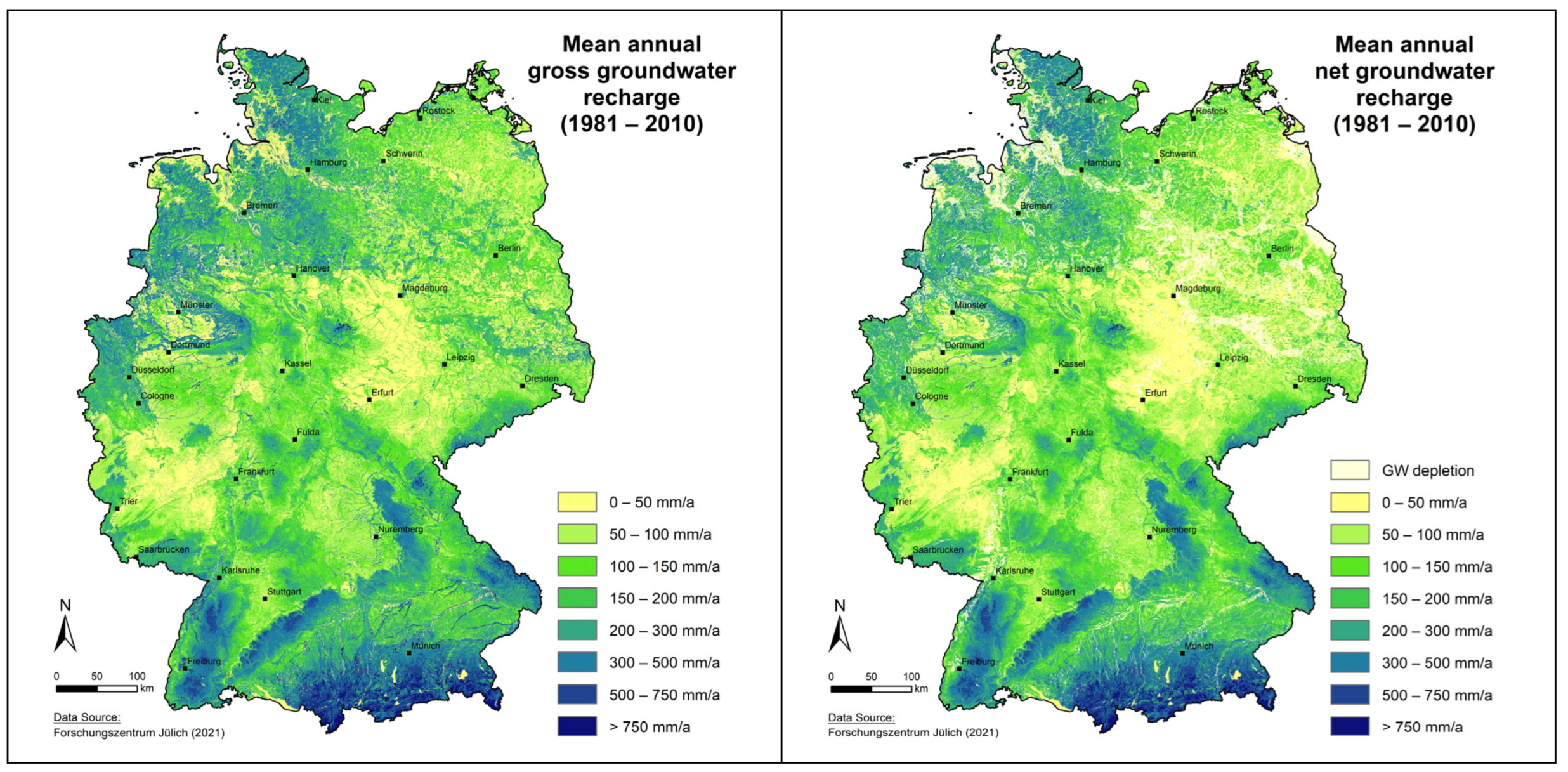
4.4. Gross and Net Groundwater Recharge

As with total runoff, a distinction is made between net groundwater recharge, which enables negative groundwater recharge due to capillary rise and direct evapotranspiration from groundwater into the root zone, and gross groundwater recharge, which does not account for these vertical upward flows from groundwater. The key parameter for calculating nutrient input to groundwater bodies and consequently groundwater-borne nutrient discharge to surface waters is the gross groundwater recharge (Figure 8, left). However, the distinction between net (Figure 8, right) and gross groundwater recharge should not obscure the fact that groundwater recharge in most regions of Germany is unaffected by near-surface groundwater, so net and gross groundwater recharge are identical.

Regions in southern Germany such as the Alpine foothills or the Black Forest exhibit high groundwater recharge above 300 mm/a, mainly due to the high annual precipitation (>1200 mm/a). In the Swabian-Franconian Jura, and northwestern Germany, precipitation may be lower, but a higher percentage of the leachate contributes to groundwater recharge.

In most bedrock regions, mean annual groundwater recharge quantities are less than 100 mm/a. Due to the low water storage capacity of the Paleozoic slate rock sequences of the Rhenish Slate Mountains, groundwater recharge of 100 mm/a is not exceeded despite high annual precipitation. Groundwater recharge in the same order of magnitude is also modelled for the fine-grained Mesozoic rock sequences (e.g., marl rocks of the Münsterland Basin). Groundwater recharge of less than 50 mm/a is also widespread in the South German stratified plain and the Thuringian Basin, but in these regions, low precipitation is a driving factor.

In unconsolidated rock areas without near-surface groundwater (Upper Rhine Plain, North German Plain) and some larger river valleys, all of the leachate can infiltrate into the aquifer. When precipitation exceeds 800 mm/a, as is the case in the western part of the North German Plain, groundwater recharge of up to 300 mm/a can be reached. Over areas with lower annual precipitation, such as the Lower Rhine Embayment, groundwater recharge of approximately 200 mm/a occurs. However, in the eastern German states, groundwater recharge is consistently below 50 mm/a even at sites without near-surface groundwater. The main reason is the low annual precipitation (<600 mm/a).

The difference between gross and net groundwater recharge (Figure 8, right) is evident in regions with a high groundwater level, where drainage systems have been installed, such as the marshlands on the North Sea coast, but also in many groundwater-affected lowland areas in the eastern part of Germany (e.g., Spree and Havel lowlands, Uckermark). In such areas, groundwater recharge occurs only in the months when the groundwater table drops below the depth of the drainage.

5. Validation of Modelled Runoff Components

For an adequate validation of the modelled runoff components, measured time series of river discharge and delineations of the corresponding catchments are required. To validate the suitability of a model for different landscapes, the spatial distribution of the catchments used for validation should cover a wide range of land uses as well as climatic, pedological, and topographic site conditions. In addition, the runoff recorded at the gauge should cover the same period that was modelled.

For the model validation, verified daily discharge data of gauging stations for the period 1980–2010 from the database ‘HYDABA’ of the Federal Institute of Hydrology (BfG) were available for 464 gauges. Additionally, point coordinates of the individual gauges and the size of the corresponding catchments were provided from the German Hydrological Yearbook (DGJ), but no polygon shape data for the catchment delineations were available. We follow a GIS-based approach to delineate the catchments using the available gauge locations and the digital elevation model DGM25. Time series of discharge data were excluded from the validation if the location of the gauge was not reported, if discharge data exhibited implausible inconsistencies (outliers, gaps), if parts of the corresponding catchment were located outside Germany, if the corresponding catchment had an area smaller than 10 km², if the reported catchment size from DGJ varied from the size of the delineated catchment significantly, or if there was a significant anthropogenic influence. After applying these criteria, 298 catchments remained for the model validation.

Figure 9 (left) shows the spatial distribution of the discharge stations and corresponding catchments throughout Germany. Except for the northwestern part of the country, where gauges are lacking due to the influence of tides and where catchments extend outside of Germany, the model area coverage is satisfactory.

We validated the model performance for both net total runoff and net groundwater recharge. For total runoff, the mean annual simulated runoff was averaged over each catchment and then compared against the observed discharge, which was converted to an effective value of mm/a over the corresponding catchment. If satisfactory agreement is achieved for a sufficiently large number of catchments, we can assume that the model is fit for purpose.

The comparison of simulated net total runoff and observed mean annual discharges for 1981–2010 is presented in Figure 9 (top right). There is an overall good agreement between observed and simulated values, with most catchments exhibiting a bias of less than 20%. Model performance was quantified based on the statistical parameters NSE (Nash-Sutcliffe efficiency) and PBIAS (percent bias). NSE [86] indicates the approximation of simulated and modelled discharges to the 1:1 line. The closer the NSE value is to 1, the better the model performance. The PBIAS value [87] indicates the tendency of simulated runoff to be underestimated or overestimated. The closer the value is to 0, the less the model tends to overestimate or underestimate the measured total runoff. The mGROWA model is validated based on NSE and PBIAS, as described in [62,70].

The NSE of 0.89 for net total runoff demonstrates a very good fit with the observed long-term mean discharge from the gauging stations. The PBIAS of −4.0% indicates a slight overestimation of the modelled values. The fit of the model to the observed values represents a very good agreement in the context of the available data and with respect to the size and heterogeneity of the considered study area. It can be concluded that the mGROWA model, together with the inputs described in Section 3, provides realistic estimates of total runoff for Germany.

In the context of modelling nutrient inputs into groundwater or surface waters, it is crucial to ascertain whether the model adequately represents the input pathways for nutrients, i.e., the runoff components. The runoff components simulated by mGROWA include both the direct runoff components (above all, drainage runoff and natural interflow) and baseflow, which can be considered equivalent to long-term groundwater recharge within catchments. The possibility of validating modelled direct runoff at the state level is limited by the lack of official monitoring networks for the long-term recording of direct runoff components, such as drainage runoff. The only runoff component for which model validation is usually performed is groundwater recharge. For the validation of the modelled net groundwater recharge (Figure 8, right), the same 298 catchments as in the total runoff evaluation were selected (Figure 9, left). For areas in Germany where unconsolidated rocks dominate, the mean groundwater runoff is often approximated using the minimum monthly low flow [88], also known as the “Wundt method”. For this study, this applies to 80 catchments. The other 218 catchments are dominated by bedrock, for which the “Demuth method” [89] is suitable for runoff separation. Similar to the validation of net total runoff, both observed baseflow and simulated groundwater recharge are converted to estimates of mm/a over the corresponding catchments. As indicated by the NSE of 0.70 and the PBIAS of 13.9%, the agreement between the simulated net groundwater recharge and the derived baseflow (Figure 9, bottom right) is relatively good. When validating modelled groundwater recharge, error propagation can occur because both the estimation of total runoff and the subsequent flow separation affect the estimates. Therefore, it is not surprising that the performance indices show lower agreement for the simulated groundwater recharge than for the simulated total runoff. In addition, many regions in Germany have groundwater recharge of less than 150 mm/a, so small absolute deviations from the observed baseflow are sufficient to result in a deviation of more than 20% for the modelled value.

6. Discussion and Conclusions

This study has provided spatially differentiated estimates of the runoff components for the period 1981–2010, calculated using a high-resolution (100 m) hydrological model that incorporates multiple soil layers based on a fine-scale 1:200,000 soil map. Other published studies of Germany-wide hydrological modelling have a coarser spatial resolution of important input layers (e.g., soil) and model outputs (250 or 1000 m); they also cover a less recent hydrological period [90,91,92]. Furthermore, unlike the aforementioned studies, the hierarchical flow separation module incorporated in mGROWA (Figure 3) allows for: (i) the inclusion of important site characteristics, such as artificial drainage and percentage imperviousness; and (ii) total runoff to be separated into more runoff components. This differentiation of flow paths is essential for the reliable modelling of nutrient inputs. Also, the study from Huang et al. [90] is validated over only 29 large river basins, whereas we validated our model over 298 catchments of varying sizes, thus ensuring that our model exhibits a strong spatial representativeness throughout Germany. A more recent study [93] used a machine learning model to generate mean long-term groundwater recharge estimates (1 km resolution) over Europe; however, the nonexistence of training and validation data over Germany makes it difficult to assess the suitability of their results within Germany.

The daily water balance in each grid cell in mGROWA is calculated using predefined parameter values for soil properties and land cover, among other things. In contrast, lumped hydrological models are typically calibrated against total discharge, which can result in model parameters sometimes being calibrated to unrealistic values and other water balance components being affected in order to achieve good results for total discharge [94]. Therefore, an advantage of using the deterministic grid-based mGROWA model is that a feasible representation of all water balance components is achieved.

Another advantage of the mGROWA model is the ability to model in high spatial and temporal resolution while maintaining a reasonable computational time. This high spatial resolution modelling allows for small-scale features in input parameters to be adequately represented within the model grid, meaning that a higher level of reliability in the representativeness of the modelling results is ensured. Last, the simple grid-based structure of mGROWA ensures that it is easily transferable to other study areas, which is evident as the model has been successfully applied in multiple other countries (e.g., [70,78]).

On the other hand, to do justice to the high spatial resolution that can be modelled using mGROWA, the input data required also need to be available. These data are not always available at a high spatial resolution (or with high reliability) in every country, meaning that an assessment of the viability of establishing an mGROWA model in a new study area should be undertaken before building a model. Also, while the vertical processes of the water balance can be balanced with mGROWA, the individual grid cells are not linked, meaning that lateral fluxes are not considered.

When interpreting the modelled runoff values with regard to their significance for nutrient export, it should be noted that absolute values of a runoff component alone do not allow for conclusions to be drawn about its regional significance as an input pathway for nutrients. This is exemplified by sites in the North German Plain with a deep groundwater table. At these sites, gross groundwater recharge of less than 100 mm/a in the eastern part of the North German Plain (Figure 8, left) is significantly lower than in the western part of the North German Plain where values of up to 300 mm/a can occur. However, this groundwater recharge is by no means a more dominant input pathway for nitrate into groundwater in the western part of the North German Plain than in the eastern part of the North German Plain. The decisive factor for differences in groundwater recharge is the decreasing precipitation quantities in the east (Figure 4, left). The relevance of groundwater recharge as an input pathway is, however, the same for sites without near-surface groundwater in the entire North German Plain. The same is true when comparing the absolute levels of runoff components across regions. For example, the drainage runoff in the northeastern German region is generally less than 150 mm/a, yet it has the same dominance as an input pathway as the natural interflow in the Rhenish Slate Mountains, which has values up to 700 mm/a. In both of these regions, more than 70% of the runoff occurs via the discharge component described above. To understand the regionally dominant input pathways for nutrients, it is, therefore, important to consider the relative shares of the individual runoff components rather than the absolute values of the runoff components (Figure 10). Here, it becomes clear that throughout Germany, the interflow and groundwater recharge are the major input pathways where the shares of interflow are highest in the bedrock areas of southern Germany and those of groundwater recharge are highest in the North German Plain. Combined surface and urban runoff as well as drainage runoff are less widely distributed; however, they also have high shares locally, e.g., in the marsh regions near the North Sea.

The modelled total runoff and groundwater recharge for the 1981–2010 period was validated against gauge-based runoff measurements. Although we obtained a good agreement with discharge measurements, as indicated by the performance indicators, it does not necessarily mean that the water balance values modelled for individual 100 m × 100 m grid cells are representative [95]. Theoretically, it is possible that overestimations and underestimations in individual grid cells balance out at the catchment scale, resulting in the catchment-averaged simulated and observed values being similar. If, as for the modelling performed here, the goal is to represent the runoff components as spatially high-resolution input pathways for nutrients, the catchment-scale model validation is not ideal. However, monitoring systems for recording and balancing individual runoff components at discrete locations do not exist in our study area. Therefore, due to the unavailability of spatially distributed measurements in catchments, the comparison of simulated with observed discharges at the catchment outlet remains the only feasible option for model validation in many practical cases [96].

To assess the representativeness of the modelled runoff, it is important to include runoff records without strong anthropogenic influences from as many discharge stations as possible in the validation process. The 298 gauge-related catchments used for model validation are a sufficient number and have a good spatial coverage of Germany; hence, they can be regarded as a good dataset to use for the assessment of the model performance.

The only runoff component that was explicitly validated in the model and that represents an important input pathway for nutrients is groundwater recharge. The validation of direct runoff components (surface runoff, direct runoff from urban areas, drainage runoff, natural interflow) is limited because all direct runoff components enter surface waters relatively soon after a precipitation event and are difficult to separate from each other in discharge data from river gauges. Nevertheless, several conclusions can be drawn from the results of the validation process regarding the representation of input pathways for modelling nutrient fluxes. As the sum of the direct runoff components is equal to the difference between the validated net total runoff and net groundwater recharge, at least the validity of the sum of the modelled direct runoff components was confirmed. Additionally, for most regions, only one of the two main components of direct runoff, i.e., natural interflow or drainage runoff, exhibits large values (Figure 7); therefore, the result of validation for the modelled groundwater recharge can be considered as an indirect validation of the modelled natural interflow and drainage runoff in that region. Thus, validation can be regarded as representative of all major runoff components, i.e., groundwater recharge, interflow, and drainage runoff. Accordingly, we conclude that the main input pathways for nitrate were modelled in a regionally realistic and representative manner.

Since the mGROWA model operates in daily time steps, it is theoretically possible to use mGROWA model results at a high temporal resolution for the determination of nutrient input pathways and the corresponding input pathway-specific N and P loads. However, such application of mGROWA model results is not practical within the AGRUM-DE project.

Caution is advised when using the modelled runoff components that represent long-term averages for characterising short time periods because of the high interannual or even intra-annual climatic variations. Accordingly, there is a risk that modelled pathway-specific N and P loads will be driven more by regional climate variability than by regional N and P supply. For this reason, all mGROWA model results were aggregated to long-term averages for 1981–2010. This provides a reliable reference not only for determining regionally dominant input pathways but also for calculating input pathway-specific nutrient loads.

A key application of these results is to understand how nutrient reduction measures could alter the N and P inputs into groundwater or surface water. Because the temporal resolution of the nutrient supply scenarios in the AGRUM-DE project is based on multi-year moving averages [97], the long-term annual means of the runoff components presented in this paper provide a suitable reference situation for analysing these scenarios. An advantage of conducting analyses using these temporally aggregated results is that the modelled changes in the nutrient loads are exclusively due to changes in the N and P supply (e.g., fertilisation of the soils) and not due to climatic variability.

In current projects within Germany, further improvement of input datasets to the mGROWA model is ongoing (e.g., higher spatial resolution of soil data and imperviousness). In addition, the latest climatic reference period of 1991–2020 has been modelled and additional gauges included for the model validation. Here, initial runoff validation results suggest at least an equally good agreement with observed data as in the study presented here.

References

1. Tesoriero, A.J.; Duff, J.H.; Saad, D.A.; Spahr, N.E.; Wolock, D.M. Vulnerability of Streams to Legacy Nitrate Sources. Environ. Sci. Technol. 2013, 47, 3623–3629. [Google Scholar] [CrossRef]
2. Adams, R.; Quinn, P.; Barber, N.; Burke, S. Identifying Flow Pathways for Phosphorus Transport Using Observed Event Forensics and the CRAFT (Catchment Runoff Attenuation Flux Tool). Water 2020, 12, 1081. [Google Scholar] [CrossRef]
3. Song, J.-H.; Her, Y.; Guo, T. Quantifying the contribution of direct runoff and baseflow to nitrogen loading in the Western Lake Erie Basins. Sci. Rep. 2022, 12, 9216. [Google Scholar] [CrossRef]
4. Hrachowitz, M.; Savenije, H.; Bogaard, T.A.; Tetzlaff, D.; Soulsby, C. What can flux tracking teach us about water age distribution patterns and their temporal dynamics? Hydrol. Earth Syst. Sci. 2013, 17, 533–564. [Google Scholar]
5. Huffman, L.R.; Fangmeier, D.D.; Elliot, W.J.; Workman, S.R. Chapter 5: Infiltration and Runoff. In Soil and Water Conservation Engineering, 7th ed.; ASABE: St. Joseph, MI, USA, 2013; pp. 81–113. [Google Scholar]
6. Meals, D.W.; Dressing, S.A.; Davenport, T.E. Lag Time in Water Quality Response to Best Management Practices: A Review. J. Environ. Qual. 2010, 39, 85–96. [Google Scholar] [CrossRef]
7. Guo, Y.; Zhang, Y.; Zhang, T.; Wang, K.; Ding, J.; Gao, H. Surface Runoff. In Observation and Measurement of Ecohydrological Processes; Li, X., Vereecken, X., Eds.; Springer: Berlin/Heidelberg, Germany, 2019; pp. 241–306. [Google Scholar]
8. Baumgartner, A.; Liebscher, H.J. Allgemeine Hydrologie-Quantitative Hydrologie: Mit 347 Abbildungen und 126 Tabellen; Borntraeger: Stuttgart, Germany, 1996. [Google Scholar]
9. Seibert, S.P.; Auerswald, K. (Eds.) Abflussverzögerung—Wie Abfluss gebremst werden kann. In Hochwasserminderung im Ländlichen Raum: Ein Handbuch zur Quantitativen Planung; Springer: Berlin/Heidelberg, Germany, 2020; pp. 113–157. [Google Scholar]
10. Yu, B.; Rose, C.W.; Ciesiolka, C.C.A.; Cakurs, U. The relationship between runoff rate and lag time and the effects of surface treatments at the plot scale. Hydrol. Sci. J. 2000, 45, 709–726. [Google Scholar] [CrossRef]
11. Wendland, F.; Albert, H.; Bach, M.; Schmidt, R. (Eds.) Hydrologische Rasterkarten. In Atlas zum Nitratstrom in der Bundesrepublik Deutschland: Rasterkarten zu geowissenschaftlichen Grundlagen, Stickstoffbilanzgrößen und Modellergebnissen; Springer: Berlin/Heidelberg, Germany, 1993; pp. 5–17. [Google Scholar]
12. Johnes, P. Evaluation and management of the impact of land use change on the nitrogen and phosphorus load delivered to surface waters: The export coefficient modelling approach. J. Hydrol. 1996, 183, 323–349. [Google Scholar] [CrossRef]
13. Flügel, W.-A.; Smith, R. Integrated process studies and modelling simulations of hillslope hydrology and interflow dynamics using the HILLS model. Environ. Model. Softw. 1998, 14, 153–160. [Google Scholar] [CrossRef]
14. Schwarze, R.; Herrmann, A.; Münch, A.; Grünewald, U.; Schöniger, M. Rechnergestützte Analyse von Abflusskomponenten und Verweilzeiten in kleinen Einzugsgebieten. Acta Hydrophys 1991, 35, 143–184. [Google Scholar]
15. Heathwaite, A.; Burke, S.; Bolton, L. Field drains as a route of rapid nutrient export from agricultural land receiving biosolids. Sci. Total. Environ. 2006, 365, 33–46. [Google Scholar] [CrossRef]
16. DIN 4049-3; Hydrologie-Teil 3: Begriffe zur Quantitativen Hydrologie. DIN Standards: Berlin, Germany, 1994.
17. de Vries, J.J.; Simmers, I. Groundwater recharge: An overview of processes and challenges. Hydrogeol. J. 2002, 10, 5–17. [Google Scholar] [CrossRef]
18. Nigate, F.; Van Camp, M.; Yenehun, A.; Belay, A.S.; Walraevens, K. Recharge–Discharge Relations of Groundwater in Volcanic Terrain of Semi-Humid Tropical Highlands of Ethiopia: The Case of Infranz Springs, in the Upper Blue Nile. Water 2020, 12, 853. [Google Scholar] [CrossRef]
19. Piggott, A.R.; Moin, S.; Southam, C. A revised approach to the UKIH method for the calculation of baseflow / Une approche améliorée de la méthode de l’UKIH pour le calcul de l’écoulement de base. Hydrol. Sci. J. 2005, 50, 920. [Google Scholar] [CrossRef]
20. Schilling, K.E.; Langel, R.J.; Wolter, C.F.; Arenas-Amado, A. Using baseflow to quantify diffuse groundwater recharge and drought at a regional scale. J. Hydrol. 2021, 602, 126765. [Google Scholar] [CrossRef]
21. Healy, R.W. Estimating Groundwater Recharge; Cambridge University Press: Cambridge, UK, 2010. [Google Scholar]
22. Van Meter, K.J.; Basu, N.B.; Veenstra, J.J.; Burras, C.L. The nitrogen legacy: Emerging evidence of nitrogen accumulation in anthropogenic landscapes. Environ. Res. Lett. 2016, 11, 035014. [Google Scholar] [CrossRef]
23. Fleck, S.; Eickenscheidt, N.; Ahrends, B.; Evers, J.; Grüneberg, E.; Ziche, D.; Hohle, J.; Schmitz, A.; Weis, W.; Schmidt-Walter, P.; et al. Nitrogen Status and Dynamics in German Forest Soils. In Status and Dynamics of Forests in Germany: Results of the National Forest Monitoring; Wellbrock, N., Bolte, A., Eds.; Springer International Publishing: Cham, Switzerland, 2019; pp. 123–166. [Google Scholar]
24. Wendland, F.; Bergmann, S.; Eisele, M.; Gömann, H.; Herrmann, F.; Kreins, P.; Kunkel, R. Model-Based Analysis of Nitrate Concentration in the Leachate—The North Rhine-Westfalia Case Study, Germany. Water 2020, 12, 550. [Google Scholar] [CrossRef]
25. Hofstra, N.; Bouwman, A.F. Denitrification in Agricultural Soils: Summarizing Published Data and Estimating Global Annual Rates. Nutr. Cycl. Agroecosystems 2005, 72, 267–278. [Google Scholar] [CrossRef]
26. Barton, L.; McLay, C.D.A.; Schipper, L.A.; Smith, C.T. Annual denitrification rates in agricultural and forest soils: A review. Soil Res. 1999, 37, 1073–1094. [Google Scholar] [CrossRef]
27. Dusek, J.; Vogel, T. Modeling Travel Time Distributions of Preferential Subsurface Runoff, Deep Percolation and Transpiration at A Montane Forest Hillslope Site. Water 2019, 11, 2396. [Google Scholar] [CrossRef]
28. Wossenyeleh, B.K.; Verbeiren, B.; Diels, J.; Huysmans, M. Vadose Zone Lag Time Effect on Groundwater Drought in a Temperate Climate. Water 2020, 12, 2123. [Google Scholar] [CrossRef]
29. Herrmann, F.; Berthold, G.; Fritsche, J.-G.; Kunkel, R.; Voigt, H.-J.; Wendland, F. Development of a conceptual hydrogeological model for the evaluation of residence times of water in soil and groundwater: The state of Hesse case study, Germany. Environ. Earth Sci. 2012, 67, 2239–2250. [Google Scholar] [CrossRef]
30. Wolters, T.; Bach, T.; Eisele, M.; Eschenbach, W.; Kunkel, R.; McNamara, I.; Well, R.; Wendland, F. The derivation of denitrification conditions in groundwater: Combined method approach and application for Germany. Ecol. Indic. 2022, 144, 109564. [Google Scholar] [CrossRef]
31. Tetzlaff, B.; Haider, J.; Kreins, P.; Kuhr, P.; Kunkel, R.; Wendland, F. Grid-based modelling of nutrient inputs from diffuse and point sources for the state of North Rhine-Westphalia (Germany) as a tool for river basin management according to EU-WFD. River Syst. 2013, 20, 213–229. [Google Scholar] [CrossRef]
32. Reid, K.; Schneider, K.; McConkey, B. Components of Phosphorus Loss From Agricultural Landscapes, and How to Incorporate Them Into Risk Assessment Tools. Front. Earth Sci. 2018, 6, 135. [Google Scholar] [CrossRef]
33. Holman, I.P.; Whelan, M.J.; Howden, N.J.; Bellamy, P.H.; Willby, N.J.; Rivas-Casado, M.; McConvey, P. Phosphorus in groundwater—An overlooked contributor to eutrophication? Hydrol. Process. 2008, 22, 5121–5127. [Google Scholar] [CrossRef]
34. Schulla, J. Model Descripiton WaSiM; Technical report; 2021; p. 396. Available online: http://www.wasim.ch/downloads/doku/wasim/wasim_2021_en.pdf (accessed on 29 August 2023).
35. Abbott, M.B.; Bathurst, J.C.; Cunge, J.A.; O’Connell, P.E.; Rasmussen, J. An introduction to the European Hydrological System—Systeme Hydrologique Europeen, “SHE”, 1: History and philosophy of a physically-based, distributed modelling system. J. Hydrol. 1986, 87, 45–59. [Google Scholar] [CrossRef]
36. Bormann, H.; Elfert, S. Application of WaSiM-ETH model to Northern German lowland catchments: Model performance in relation to catchment characteristics and sensitivity to land use change. Adv. Geosci. 2010, 27, 1–10. [Google Scholar] [CrossRef]
37. Schäfer, C.; Fäth, J.; Kneisel, C.; Baumhauer, R.; Ullmann, T. Multidimensional hydrological modeling of a forested catchment in a German low mountain range using a modular runoff and water balance model. Front. For. Glob. Chang. 2023, 6, 1186304. [Google Scholar] [CrossRef]
38. Papadimos, D.; Demertzi, K.; Papamichail, D. Assessing Lake Response to Extreme Climate Change Using the Coupled MIKE SHE/MIKE 11 Model: Case Study of Lake Zazari in Greece. Water 2022, 14, 921. [Google Scholar] [CrossRef]
39. Wolf, J.; Beusen, A.; Groenendijk, P.; Kroon, T.; Rötter, R.; van Zeijts, H. The integrated modeling system STONE for calculating nutrient emissions from agriculture in the Netherlands. Environ. Model. Softw. 2003, 18, 597–617. [Google Scholar] [CrossRef]
40. Hansen, B.; Dalgaard, T.; Thorling, L.; Sørensen, B.; Erlandsen, M. Regional analysis of groundwater nitrate concentrations and trends in Denmark in regard to agricultural influence. Biogeosciences 2012, 9, 3277–3286. [Google Scholar] [CrossRef]
41. Rashid, M.A.; Bruun, S.; Styczen, M.E.; Ørum, J.E.; Borgen, S.K.; Thomsen, I.K.; Jensen, L.S. Scenario analysis using the Daisy model to assess and mitigate nitrate leaching from complex agro-environmental settings in Denmark. Sci. Total. Environ. 2022, 816, 151518. [Google Scholar] [CrossRef]
42. Henriksen, H.J.; Troldborg, L.; Nyegaard, P.; Sonnenborg, T.O.; Refsgaard, J.C.; Madsen, B. Methodology for construction, calibration and validation of a national hydrological model for Denmark. J. Hydrol. 2003, 280, 52–71. [Google Scholar] [CrossRef]
43. Chen, L.; Šimůnek, J.; Bradford, S.A.; Ajami, H.; Meles, M.B. A computationally efficient hydrologic modeling framework to simulate surface-subsurface hydrological processes at the hillslope scale. J. Hydrol. 2022, 614, 128539. [Google Scholar] [CrossRef]
44. Díaz, I.; Levrini, P.; Achkar, M.; Crisci, C.; Nion, C.F.; Goyenola, G.; Mazzeo, N. Empirical Modeling of Stream Nutrients for Countries without Robust Water Quality Monitoring Systems. Environments 2021, 8, 129. [Google Scholar] [CrossRef]
45. Kreins, P.; Gömann, H.; Herrmann, S.; Kunkel, R.; Wendland, F. Integrated Agricultural and Hydrological Modeling within an Intensive Livestock Region. In Ecological Economics of Sustainable Watershed Management; Erickson, J.D., Messner, F., Ring, I., Eds.; Emerald Group Publishing Limited: Bingley, UK, 2007; pp. 113–142. [Google Scholar]
46. Arnold, J.G.; Srinivasan, R.; Muttiah, R.S.; Williams, J.R. Large Area hydrologic modeling and assessment Part I: Model Development. JAWRA J. Am. Water Resour. Assoc. 1998, 34, 73–89. [Google Scholar] [CrossRef]
47. Tetzlaff, B.; Vereecken, H.; Kunkel, R.; Wendland, F. Modelling phosphorus inputs from agricultural sources and urban areas in river basins. Environ. Geol. 2009, 57, 183–193. [Google Scholar] [CrossRef]
48. Arheimer, B.; Dahné, J.; Donnelly, C.; Lindström, G.; Strömqvist, J. Water and nutrient simulations using the HYPE model for Sweden vs. the Baltic Sea basin—Influence of input-data quality and scale. Hydrol. Res. 2012, 43, 315–329. [Google Scholar] [CrossRef]
49. Kunkel, R.; Herrmann, F.; Kape, H.-E.; Keller, L.; Koch, F.; Tetzlaff, B.; Wendland, F. Simulation of terrestrial nitrogen fluxes in Mecklenburg-Vorpommern and scenario analyses how to reach N-quality targets for groundwater and the coastal waters. Environ. Earth Sci. 2017, 76, 146. [Google Scholar] [CrossRef]
50. EEC. Council Directive 91/676/EEC of 12 December 1991 concerning the protection of waters against pollution caused by nitrates from agricultural sources. Off. J. Eur. Communities 1991, 375, 1–8. [Google Scholar]
51. EU-WFD. Directive 2000/60/EC of the European Parliament and of the Council of 23 October 2000 establishing a framework for Community action in the field of water policy. Off. J. Eur. Communities 2000, 327, 1–73. [Google Scholar]
52. EU-MSFD. Directive 2008/56/EC of the European Parliament and of the Council of 17 June 2008 establishing a framework for community action in the field of marine environmental policy. Off. J. Eur. Communities 2008, 26, 1–40. [Google Scholar]
53. Heidecke, C.H.U.; Kreins, P.; Kuhr, P.; Kunkel, R.; Mahnkopf, J.; Schott, M.; Tetzlaff, B.; Venohr, M.; Wagner, A. Endbericht zum Forschungsprojekt “Entwicklung eines Instrumentes für ein flussgebietsweites Nährstoffmanagement in der FlussgebietseinheitWeser” AGRUM+-Weser; Johann Heinrich von Thünen-Institut: Braunschweig, Germany, 2015; p. 380. [Google Scholar]
54. Wendland, F.B.H.; Hirt, U.; Kreins, P.; Kuhn, U.; Kuhr, P.; Kunkel, R.; Tetzlaff, B. Analyse von Agrar- und Umweltmaßnahmen zur Reduktion der Stickstoffbelastung von Grundwasser und Oberflächengewässer in der Flussgebietseinheit Weser. Hydrol. Und Wasserbewirtsch. 2010, 54, 231–244. [Google Scholar]
55. Henrichsmeyer, W.; Cypris, C.; Löhe, W.; Meudt, M.; Sander, R.; v Sothen, F. Entwicklung des Gesamtdeutschen Agrarsektormodells RAUMIS96. Endbericht Zum Kooperationsprojekt; Institut für Agrarpolitik, Marktforschung und Wirtschaftssoziologie der Universität Bonn: Bonn, Germany, 1996. [Google Scholar]
56. Wolters, T.; Cremer, N.; Eisele, M.; Herrmann, F.; Kreins, P.; Kunkel, R.; Wendland, F. Checking the Plausibility of Modelled Nitrate Concentrations in the Leachate on Federal State Scale in Germany. Water 2021, 13, 226. [Google Scholar] [CrossRef]
57. Herrmann, F.; Keller, L.; Kunkel, R.; Vereecken, H.; Wendland, F. Determination of spatially differentiated water balance components including groundwater recharge on the Federal State level—A case study using the mGROWA model in North Rhine-Westphalia (Germany). J. Hydrol. Reg. Stud. 2015, 4, 294–312. [Google Scholar] [CrossRef]
58. Behrendt, H.; Kornmilch, M.; Opitz, D.; Schmoll, O.; Scholz, G. Estimation of the nutrient inputs into river systems-experiences from German rivers. Reg. Environ. Chang. 2002, 3, 107–117. [Google Scholar] [CrossRef]
59. Venohr, M.; Hirt, U.; Hofmann, J.; Opitz, D.; Gericke, A.; Wetzig, A.; Natho, S.; Neumann, F.; Hürdler, J.; Matranga, M.; et al. Modelling of Nutrient Emissions in River Systems-MONERIS-Methods and Background. Int. Rev. Hydrobiol. 2011, 96, 435–483. [Google Scholar] [CrossRef]
60. Nguyen, H.H.; Venohr, M.; Gericke, A.; Sundermann, A.; Welti, E.A.; Haase, P. Dynamics in impervious urban and non-urban areas and their effects on run-off, nutrient emissions, and macroinvertebrate communities. Landsc. Urban Plan. 2023, 231, 104639. [Google Scholar] [CrossRef]
61. Herrmann, F. Zeitlich und räumlich hochaufgelöste flächendifferenzierte Simulation des Landschaftswasserhaushalts in Niedersachsen mit dem Model mGROWA. Hydrol Wasserbewirtsch 2013, 57, 206–224. [Google Scholar]
62. Herrmann, F.; Engel, N.; Wendland, F.; Hübsch, L.; Vereecken, H.; Müller, U.; Ostermann, U. Auswirkung von möglichen Klimaänderungen auf die Grundwasserneubildung und den Bewässerungsbedarf in der Metropolregion Hamburg. In Proceedings of the 10. Deutsche Klimatagung, Hamburg, Germany, 21–24 September 2015. [Google Scholar]
63. Friesland, H.; Löpmeier, F.-J. The performance of the model AMBAV for evapotranspiration and soil moisture on Müncheberg data. In Modelling Water and Nutrient Dynamics in Soil–Crop Systems; Springer: Dordrecht, The Netherlands, 2007; pp. 19–26. [Google Scholar]
64. Löpmeier, F.-J. Berechnung der Bodenfeuchte und Verdunstung mittels agrarmeteorologischer Modelle. Z. Für Bewässerungswirtschaft 1994, 29, 157–167. [Google Scholar]
65. Allen, R.G.; Pereira, L.S.; Raes, D.; Smith, M. Crop evapotranspiration-Guidelines for computing crop water requirements-FAO Irrigation and drainage paper 56. Fao Rome 1998, 300, D05109. [Google Scholar]
66. Kunkel, R.; Wendland, F. The GROWA98 model for water balance analysis in large river basins—The river Elbe case study. J. Hydrol. 2002, 259, 152–162. [Google Scholar] [CrossRef]
67. Disse, M. Modellierung der Verdunstung und der Grundwasserneubildung in ebenen Einzugsgebieten. In Hydrologie und Wasserwirtschaft; Institut für Umweltingenieurwissenschaften: Karlsruhe, Germany, 1995. [Google Scholar]
68. Engel, N.M.U.; Schäfer, W. BOWAB—Ein Mehrschicht-Bodenwasserhaushaltsmodell. In Klimawandel und Bodenwasserhaushalt. GeoBerichte; Landesamt für Bergbau, Energie und Geologie: Hannover, Germany, 2012; pp. 85–98. [Google Scholar]
69. Hermann, F.W.F. Modellierung des Wasserhaushalts in Nordrhein-Westfalen mit mGROWA. Teil IIa. LANUV-Fachbericht 110. Kooperationsprojekt GROWA+ NRW 2021; Landesamt für Natur, Umwelt und Verbraucherschutz Nordrhein-Westfalen: Recklinghausen, Germany, 2021. [Google Scholar]
70. Pisinaras, V.; Herrmann, F.; Panagopoulos, A.; Tziritis, E.; McNamara, I.; Wendland, F. Fully Distributed Water Balance Modelling in Large Agricultural Areas—The Pinios River Basin (Greece) Case Study. Sustainability 2023, 15, 4343. [Google Scholar] [CrossRef]
71. Heathwaite, A.; Quinn, P.; Hewett, C. Modelling and managing critical source areas of diffuse pollution from agricultural land using flow connectivity simulation. J. Hydrol. 2005, 304, 446–461. [Google Scholar] [CrossRef]
72. Schroers, S.; Eiff, O.; Kleidon, A.; Scherer, U.; Wienhöfer, J.; Zehe, E. Morphological controls on surface runoff: An interpretation of steady-state energy patterns, maximum power states and dissipation regimes within a thermodynamic framework. Hydrol. Earth Syst. Sci. 2022, 26, 3125–3150. [Google Scholar] [CrossRef]
73. United States. Soil Conservation Service. Section 4: Hydrology. In SCS National Engineering Handbook; The Service; University of Minnesota: Minneapolis, MS, USA, 1958. [Google Scholar]
74. Bloomfield, J.; Allen, D.; Griffiths, K. Examining geological controls on baseflow index (BFI) using regression analysis: An illustration from the Thames Basin, UK. J. Hydrol. 2009, 373, 164–176. [Google Scholar] [CrossRef]
75. Wendland, F.; Kunkel, R.; Tetzlaff, B.; Dorhofer, G. GIS-based determination of the mean long-term groundwater recharge in Lower Saxony. Environ. Geol. 2003, 45, 273–278. [Google Scholar] [CrossRef]
76. Lacey, G.; Grayson, R. Relating baseflow to catchment properties in south-eastern Australia. J. Hydrol. 1998, 204, 231–250. [Google Scholar] [CrossRef]
77. Dörhöfer, G.; Josopait, V. Eine Methode zur flächendifferenzierten Ermittlung der Grundwasserneubildungsrate. Geol. Jahrb. 1980, 27, 45–65. [Google Scholar]
78. Ehlers, L.; Herrmann, F.; Blaschek, M.; Duttmann, R.; Wendland, F. Sensitivity of mGROWA-simulated groundwater recharge to changes in soil and land use parameters in a Mediterranean environment and conclusions in view of ensemble-based climate impact simulations. Sci. Total Environ. 2016, 543, 937–951. [Google Scholar] [CrossRef]
79. Panagopoulos, A.; Arampatzis, G.; Kuhr, P.; Kunkel, R.; Tziritis, E.; Wendland, F. Area-Differentiated modeling of water balance in Pinios River Basin, central Greece. Glob. Nest J. 2015, 17, 221–235. [Google Scholar]
80. Tetzlaff, B.; Andjelov, M.; Kuhr, P.; Uhan, J.; Wendland, F. Model-based assessment of groundwater recharge in Slovenia. Environ. Earth Sci. 2015, 74, 6177–6192. [Google Scholar] [CrossRef]
81. Haberlandt, U.; Klöcking, B.; Krysanova, V.; Becker, A. Regionalisation of the base flow index from dynamically simulated flow components—A case study in the Elbe River Basin. J. Hydrol. 2001, 248, 35–53. [Google Scholar] [CrossRef]
82. Herrmann, F.; Keuler, K.; Wolters, T.; Bergmann, S.; Eisele, M.; Wendland, F. Mit der Modellkette RCP-GCM-RCM-mGROWA projizierte Grundwasserneubildung als Datenbasis für zukünftiges Grundwassermanagement in Nordrhein-Westfalen. Grundwasser 2021, 26, 17–31. [Google Scholar] [CrossRef]
83. Tetzlaff, B.; Kuhr, P.; Vereecken, H.; Wendland, F. Aerial photograph-based delineation of artificially drained areas as a basis for water balance and phosphorus modelling in large river basins. Phys. Chem. Earth Parts A/B/C 2009, 34, 552–564. [Google Scholar] [CrossRef]
84. Tetzlaff, B.; Kuhr, P.; Wendland, F. A new method for creating maps of artificially drained areas in large river basins based on aerial photographs and geodata. Irrig. Drain. 2008, 58, 569–585. [Google Scholar] [CrossRef]
85. Dörhöfer, G.; Röhm, H. Aufbruch nach Europa-Hydrogeologie vor neuen Aufgaben.-Der natürliche Grundwasserhaushalt in Niedersachsen. In Arbeitshefte-Wasser; Schweizerbart Science: Stuttgart, Germany, 2001; p. 167. [Google Scholar]
86. Nash, J.E.; Sutcliffe, J.V. River flow forecasting through conceptual models part I—A discussion of principles. J. Hydrol. 1970, 10, 282–290. [Google Scholar] [CrossRef]
87. Gupta Hoshin, V.; Sorooshian, S.; Yapo Patrice, O. Status of Automatic Calibration for Hydrologic Models: Comparison with Multilevel Expert Calibration. J. Hydrol. Eng. 1999, 4, 135–143. [Google Scholar] [CrossRef]
88. Wundt, W. Die Kleinstwasserführung der Flüsse als Maß für die Verfügbaren Grundwassermengen; Scientific Research: Atlanta, GA, USA, 1958. [Google Scholar]
89. Demuth, S. Untersuchungen zum Niedrigwasser in West-Europa. In Freiburger Schriften zur Hydrologie; Institut für Hydrologie: Hannover, Germany; Universität Freiburg: Freiburg, Germany, 1993; p. 205. [Google Scholar]
90. Huang, S.; Krysanova, V.; Österle, H.; Hattermann, F.F. Simulation of spatiotemporal dynamics of water fluxes in Germany under climate change. Hydrol. Process. 2010, 24, 3289–3306. [Google Scholar] [CrossRef]
91. BMUV. Hydrologischer Atlas von Deutschland; Bundesministerium für Umwelt, Naturschutz und Reaktorsicherheit: Berlin, Germany, 2001. [Google Scholar]
92. Bundesanstalt für Geowissenschaften und Rohstoffe (BGR). BODENWASSERHAUSHALT V1.0, B.f.G.u.R. (BGR), Editor. 2017: Hannover, Germany. MUNIS. Das niedersächsische Umweltportal. Available online: https://numis.niedersachsen.de/trefferanzeige?docuuid=1756a8e6-854b-46dc-9262-310c07efadda (accessed on 29 August 2023).
93. Martinsen, G.; Bessiere, H.; Caballero, Y.; Koch, J.; Collados-Lara, A.J.; Mansour, M.; Sallasmaa, O.; Pulido-Velazquez, D.; Williams, N.H.; Zaadnoordijk, W.J.; et al. Developing a pan-European high-resolution groundwater recharge map–Combining satellite data and national survey data using machine learning. Sci. Total. Environ. 2022, 822, 153464. [Google Scholar] [CrossRef]
94. Baez-Villanueva, O.M.; Zambrano-Bigiarini, M.; Mendoza, P.A.; McNamara, I.; Beck, H.E.; Thurner, J.; Nauditt, A.; Ribbe, L.; Thinh, N.X. On the selection of precipitation products for the regionalisation of hydrological model parameters. Hydrol. Earth Syst. Sci. 2021, 25, 5805–5837. [Google Scholar] [CrossRef]
95. Sidle, R.C. Strategies for smarter catchment hydrology models: Incorporating scaling and better process representation. Geosci. Lett. 2021, 8, 24. [Google Scholar] [CrossRef]
96. Rosso, R. An introduction to spatially distributed modelling of basin response. In Advances in Distributed Hydrology; Rosso, R., Peano, A., Becchi, I., Bemporad, G.A., Eds.; Water Resources Publications: Littleton, CO, USA, 1994; pp. 3–30. [Google Scholar]
97. Zinnbauer, M.; Eysholdt, M.; Henseler, M.; Herrmann, F.; Kreins, P.; Kunkel, R.; Nguyen, H.; Tetzlaff, B.; Venohr, M.; Wolters, T.; et al. Quantifizierung Aktueller und Zukünftiger Nährstoffeinträge und Handlungsbedarfe für ein Deutschlandweites Nährstoffmanagement-AGRUM-DE; Thünen-Report; Johann Heinrich von Thünen-Institut: Braunschweig, Germany, 2023. [Google Scholar]
Figure 1. Components of total runoff.
Water 15 03468 g001
Figure 2. Determination of runoff components [62] (modified).
Water 15 03468 g002
Figure 3. Hierarchical model for the separation of runoff into the direct runoff components and groundwater recharge [57] (modified).
Water 15 03468 g003
Figure 4. Mean annual precipitation (1981–2010) (left) and locations of rain gauges with data available for the period 1981–2010 (right).
Water 15 03468 g004
Figure 5. Mean annual gross (left) and net (right) total runoff (1981–2010).
Water 15 03468 g005
Figure 6. Mean annual (1981–2010) surface runoff for the grid cells with water connection (left) and direct runoff from urban areas (right).
Water 15 03468 g006
Figure 7. Mean annual (1981–2010) natural interflow (left) and drainage runoff (right).
Water 15 03468 g007
Figure 8. Mean annual (1981–2010) gross (left) and net (right) groundwater recharge.
Water 15 03468 g008
Figure 9. Spatial distribution of gauges and their corresponding catchments used for model validation (left); comparison of the zonal mean of simulated net total runoff and observed total runoff (top right); and comparison of the zonal mean of simulated net groundwater recharge and estimated groundwater recharge from baseflow separation (bottom right).
Water 15 03468 g009
Figure 10. Percentage shares of surface and urban runoff (a), drainage runoff (b), natural interflow (c), and groundwater recharge (d) in total runoff.
Water 15 03468 g010