Using Wavelet Analysis to Examine Long-Term Variability of Phytoplankton Biomass in the Tropical, Saline Lake Alchichica, Mexico

Abstract

The phytoplankton biomass (chlorophyll-a, Chl-a) is directly related to the total production of lakes. Chl-a in temperate lakes oscillates on an annual scale. However, Chl-a oscillations in tropical lakes have hardly been documented, particularly over multiple years. Here, we described the periodicity of the Chl-a by performing a continuous wavelet analysis of 21 years (1998–2018), monthly Chl-a data from tropical, saline Lake Alchichica, Mexico. Parallel wavelet analyses were made on environmental time series (i.e., euphotic zone, mixed layer, temperature, dissolved oxygen concentration, dissolved inorganic nitrogen, soluble reactive phosphorus, soluble reactive silica). Throughout the time series, the wavelet transforms identified a regular and predictable annual cycle of the Chl-a associated with the warm-monomictic thermal-mixing pattern, the variability of the annual Chl-a cycle, and the presence of other cyclicities, 2-year and ~4–5 years, associated with external forcing agents (e.g., North Pacific Oscillation). The water quality variables display a recurrent annual cycle. At the same time, the trophic variables (nutrient concentration) showed the same cyclicity as Chl-a (1-year, 2-year, and 4-year), suggesting the external forcing agents promote Chl-a augment through nutrient increase made available from stronger, deeper, mixing periods.

1. Introduction

Phytoplankton biomass, expressed as chlorophyll-a (Chl-a), is directly related to the total production of lakes [1] and can be used as a proxy for primary production [2]. Spatial and temporal changes in Chl-a are primarily controlled by light, temperature, and nutrients in the water column. These factors also determine the phytoplankton’s size spectrum and species composition [3,4]. The annual phytoplankton succession was well documented in deep, thermally stratified temperate lakes (the Plankton Ecology Group model, e.g., [5,6]), with a unimodal phytoplankton maximum in the spring in oligotrophic lakes due to nutrient limitation.

Although many studies examined the phytoplankton variability within years, and more recently, a few long-term phytoplankton data are becoming available, few studies encompass datasets of several years or decades, primarily due to the lack of data [7]. The absence of long-term phytoplankton data and lack of continuity in records is common for tropical lakes [8,9]. According to Talling [10], the annual patterns of phytoplankton seasonality in the tropical belt are dominated by hydrological features (water inputs–outputs) or by hydrographic ones (water-column structure and circulation). Lewis [11] mentioned that in tropical lakes, the changes in phytoplankton abundance could be driven autogenically, as the organisms modify their environment (e.g., through nutrient uptake) or allogenically, associated with abiotic influences (e.g., water column mixing). Phytoplankton biomass in large tropical lakes varies at different time scales from seasons to centuries [12]. The seasonal scale in the tropics is driven by the alternation between the rainy (warm) and dry (cold) periods. In contrast, the global climate (e.g., El Niño Southern Oscillation, the Pacific Decadal Oscillation) drives the long-term scale. Despite the apparent “endless summer” [13] in tropical inland waters, there is commonly one event of deep water-column mixing, but also other different time-variability patterns (period/frequency and amplitude/range) such as the diel (24 h) cycle, the annual cycles with other periodicities (lunar, seiches, sunspots), and long-term and aperiodic or non-seasonal environmental changes [4,14].

Annual phytoplankton patterns differ across ecosystems, have large year-to-year variability [15,16,17], and are not strongly expressed in all aquatic ecosystems [18,19]. Whereas high variability of seasonal phytoplankton patterns is documented, no systematic analysis of annual cycles has been conducted to identify their characteristic periods of biomass variability and the recurrence strength at those periods [20].

Wavelet analysis performs a time-frequency analysis of the signal, which permits the estimation of the spectral characteristics of the signal as a function of time [21] and then the identification of different periodic components and their time evolution all along with the time series. Wavelet transforms are useful tools for determining the dominant scales of variation in time series and are used to examine periodicities in plankton communities [15,18,20]. However, this approach has been scarcely applied in tropical limnology.

In this work, our main goal was to reveal the variability in the annual periodicity of the phytoplankton Chl-a over 21 years and relate the variability with the environmental variables in the tropical saline Lake Alchichica, Puebla, Mexico. For this purpose, we addressed the following research questions: What are the cyclicity periods throughout 21 years (1998–2018) of (1) water quality and trophic status and (2) Phytoplankton Chl-a?

Our working hypothesis was that in this tropical, saline lake, the warm-monomictic thermal mixing pattern is the key factor determining the phenology of the pelagic Chl-a concentration. Specifically, we expected (1) to identify a predictable and recurrent annual cycle and (2) to unravel longer-term cyclicity. In order to answer the research questions and test the proposed hypothesis, our approach was to evaluate the temporal, long-term changes using data derived from monthly monitoring of the water column for 21 years (1998–2018) in the (a) water quality and trophic status and (b) phytoplankton Chl-a.

2. Materials and Methods

2.1. Study Area

Lake Alchichica is a volcanic maar in Puebla State (19°24.7′ N, 97°24.0′ W, 2300 m above the sea level), at the easternmost portion of the Mexican Plateau [22] (Figure 1).

The climate is temperate and semi-arid with an average temperature of 12.9 °C, rainfall < 500 mm year⁻¹, concentrated in the (“summer”) rainy season, and evapotranspiration rate up to 1690 mm year⁻¹ [3]. It is a deep lake (maximum depth 62 m, mean depth 40.9 m), circular in shape (maximum length 1902 m), with a surface area of 2.367 km², a shoreline of 5.84 km, and a volume of 114,688,900 m³ [23]. The lake is saline (total dissolved solids = 10.08 g L⁻¹, electrical conductivity = 13.53 mS cm⁻¹) with chloride, bicarbonate, sodium, and magnesium as dominant ions and an alkaline pH (8.7–9.2) [22,24]. Alchichica is a warm monomictic lake that circulates during the cold, dry season, from the end of December or the beginning of January to the end of March or the beginning of April. The lake remains stratified throughout the warm rainy season, and the hypolimnion becomes anoxic for most of this period [22]. Lake Alchichica is oligotrophic with an overall nutrient concentration of <4 µmol L⁻¹ at the mixed layer [25].

Nineteen species compose the phytoplankton community in Lake Alchichica, with diatoms the most diverse group with ten species. The annual phytoplankton dynamics display three characteristic features: (1) a winter diatom bloom during the mixing season, (2) a cyanobacterial bloom at the onset of the stratification period, and (3) a deep chlorophyll maximum (DCM) along the stratification period [26].

The phytoplankton biomass in Lake Alchichica is dominated (>70%) by large-sized individuals [3] corresponding to Cyclotella alchichicana Oliva, Lugo, Alcocer and Cantoral-Uriza, 2006; C. choctawhatcheeana Prasad, 1990; Chaetoceros elmorei Boyer, 1914; and Nodularia aff. spumigena Mertens ex Bornet and Flahault, 1888). Among these species, the large (35–63 μm in diameter) diatom C. alchichicana [27] comprised most of the phytoplankton biomass. It dominated the winter diatom bloom and the DCM during the stratification period, except for a brief period at the onset of the stratification when Nodularia aff. spumigena bloomed [28].

2.2. Physical, Chemical, and Chl-a Characterisation

The long-term database herein analyzed comprises a monthly sampling program made over 21 years (1998–2018) for Chl-a, euphotic zone, temperature, and dissolved oxygen in the mixed layer, and over 20 years (1999–2018) for nutrients. All samplings were made at the same station, located in the central and deepest part of the lake, and at the same time (12–13 h).

Vertical photosynthetically active radiation (PAR) and natural fluorescence profiles were recorded with a Biospherical natural fluorescence profiler model PNF-300. The profiles consisted of discrete readings recorded every second as the sensor was lowered at about 1 m per 3–4 s, providing a vertical resolution of 25–30 cm. PAR profiles were used to identify the depth of the euphotic zone (Z_EU = 0.1% surface PAR). Vertical water temperature and dissolved oxygen profiles were recorded with water quality monitoring probes (Hydrolab Datasonde models DS3, DS4, or DS5) with a vertical resolution of 1 m. Temperature and dissolved oxygen (DO) profiles were used to recognize the main stages of the lake’s thermal regime (stratification and mixing) and to identify the depth of the mixed layer (Z_MIX).

Chlorophyll-a concentration (mg m⁻³) was calculated from the natural fluorescence flux, F_f, and the incident irradiance. The natural fluorescence of Chl-a is defined as the total flux of light emitted by Chl-a in a suspension of phytoplankton per unit volume under ambient light. Keifer et al. [29] and Chamberlain et al. [30] showed that measurements of natural fluorescence flux (F_f) and scalar irradiance of PAR (E_o (PAR)) provide accurate estimates of Chl-a.

Chl-a = F_f ÷ ^oa_c (PAR) × φ_f × E_o (PAR)

The natural fluorescence records of the first five surface meters were omitted since the algorithms (from the profiler software) used to calculate the concentration of Chl-a from the natural fluorescence interpret that all the flow of red light directed upwards comes from Chl-a fluorescence. However, near the water’s surface (the first five meters in transparent waters such as Alchichica), this interpretation is incorrect due to the dispersion of the red wavelength [29].

There are two important optical assumptions used in this: ^oa_c (PAR) is the chlorophyll-specific absorption coefficient (absorption normalized to chlorophyll concentration), and φ_f is the quantum yield of fluorescence. These values are treated as constants in the software for the PNF-300 with values of 0.04 m² mg⁻¹ and 0.045 mE fluoresced per mE absorbed, respectively. The Chl-a concentration profiles were integrated per unit area (m²) to calculate the total Chl-a concentration per m².

Ten water samples along the vertical profile were obtained for nutrient analysis at each sampling date (5-L Uwitec water sampler bottle). Water samples were filtered through mixed cellulose esters syringe filters (0.22-μm pore, Millex, Millipore, Ireland), collected in polypropylene containers, and stored frozen until analysis (within 48 h). Analyses of dissolved inorganic nitrogen (DIN = NH₄⁺ + NO₂⁻ + NO₃⁻), soluble reactive phosphorus (SRP), and soluble reactive silica (SRSi) used a segmented-flow Autoanalyzer (Skalar San Plus System, Skalar Analytical B.V., Breda, The Netherlands) following Hansen and Koroleff [31].

Before wavelet analysis, we performed a seasonally-adjusted Mann–Kendall Trend Test to account for any seasonality in the phytoplanktonic chlorophyll-a concentration (1998–2018), water quality (1998–2018), and trophic (1999–2018) variables of Lake Alchichica. Analyses were run in R-4.0.3 [32].

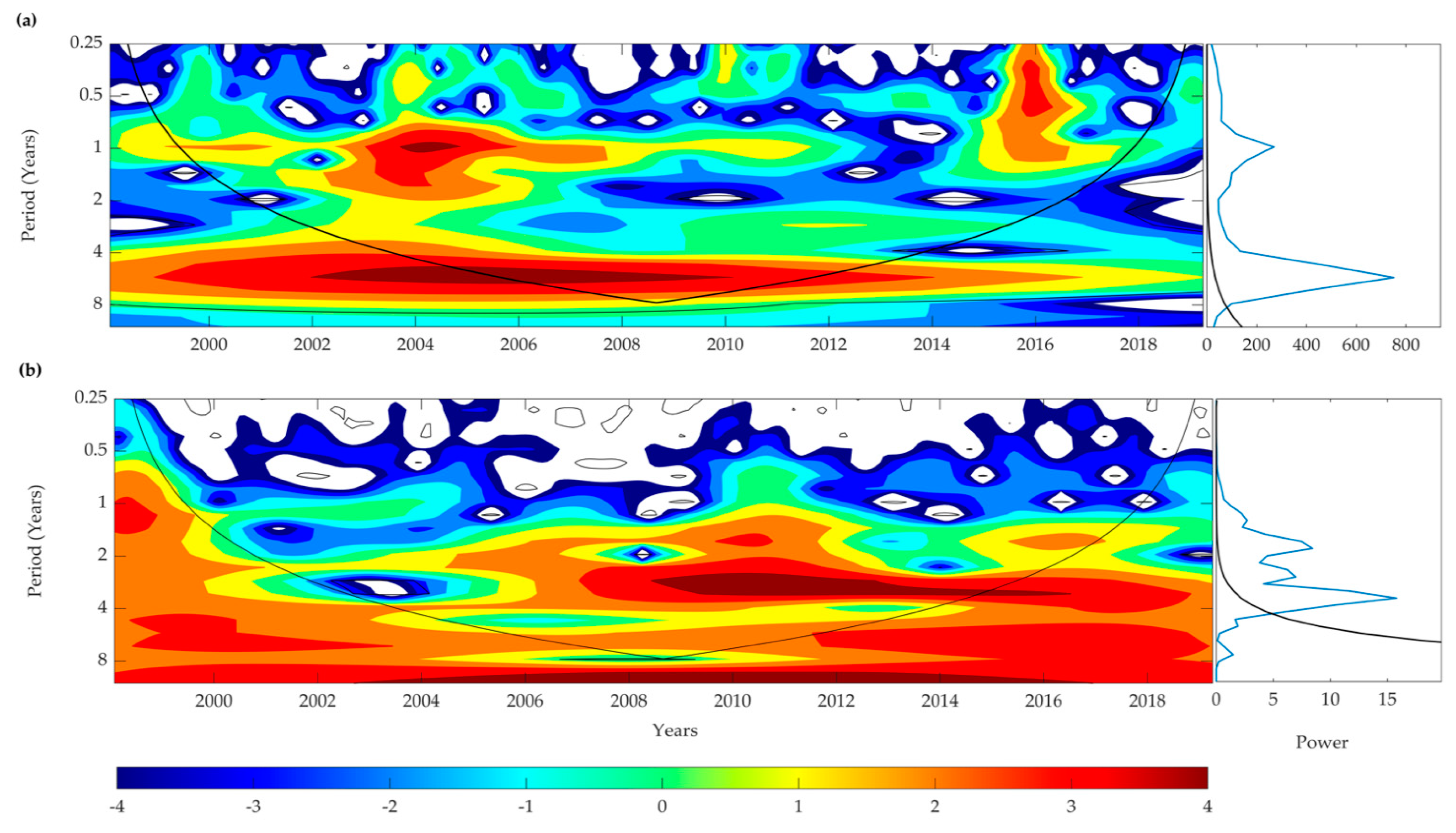
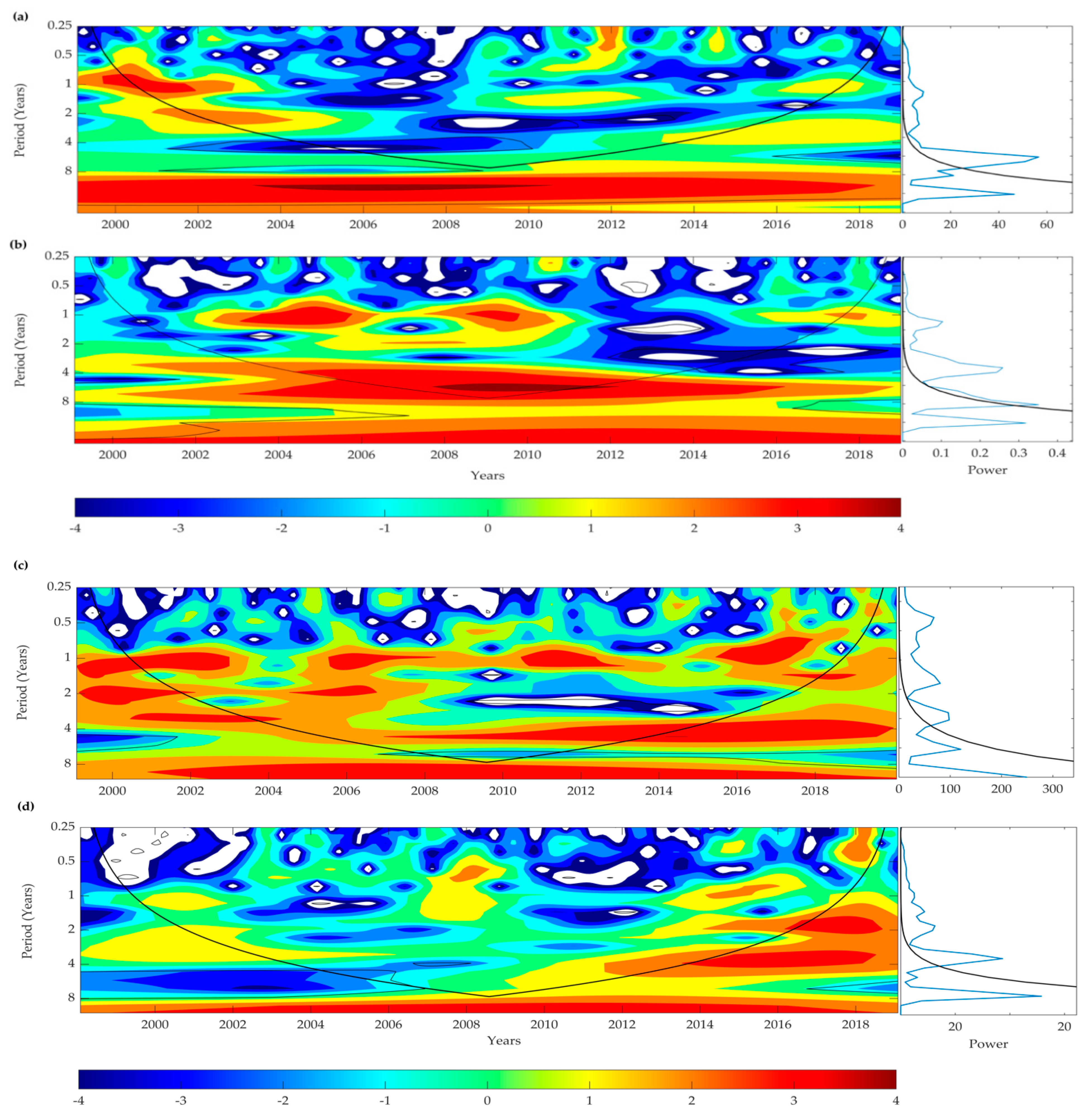
2.3. Wavelet Analysis

Wavelet analysis used continuous wavelet transforms to determine the dominant scales of variability for Chl-a, physical and chemical time series from 1998 to 2018 as a function of period and time. Wavelet analysis emerged as a tool for characterizing periodicities in non-stationary time series, as it decomposes a time series in both the frequency and time domains [33]. The latter is why it has become an important tool to analyze time series since it performs a time-frequency analysis of a signal, allowing the estimation of the spectral characteristics of the signal as a function of time [21,34], and at the same time, identifies the different periodic components and their time evolution over time. The use of wavelet analysis in aquatic ecology has increased over the last few years, especially in marine ecology. Wavelet transforms are useful tools for determining the dominant scales of variation in time series and are increasingly used to examine the periodicities in plankton (e.g., [15,20]) and other aquatic communities. Wavelet analysis performs a time-scale decomposition of the signal by estimating its frequency characteristics as a function of time [20,35].

The continuous Morlet wavelet transform was used to normalize monthly time series data and obtain the wavelet power spectrum of the time series. The wavelet power spectrum identifies the periods that are the most important sources of variability across time. In addition, it is possible to obtain a global wavelet spectrum, which is similar to Fourier spectra, that identifies the variance associated with each period for a given time series [33]. Due to the nature of the data, the original time series is not equally spaced and was made regular using spline interpolation. All the analyses for spline interpolations and wavelet transforms were performed using Matlab.

3. Results

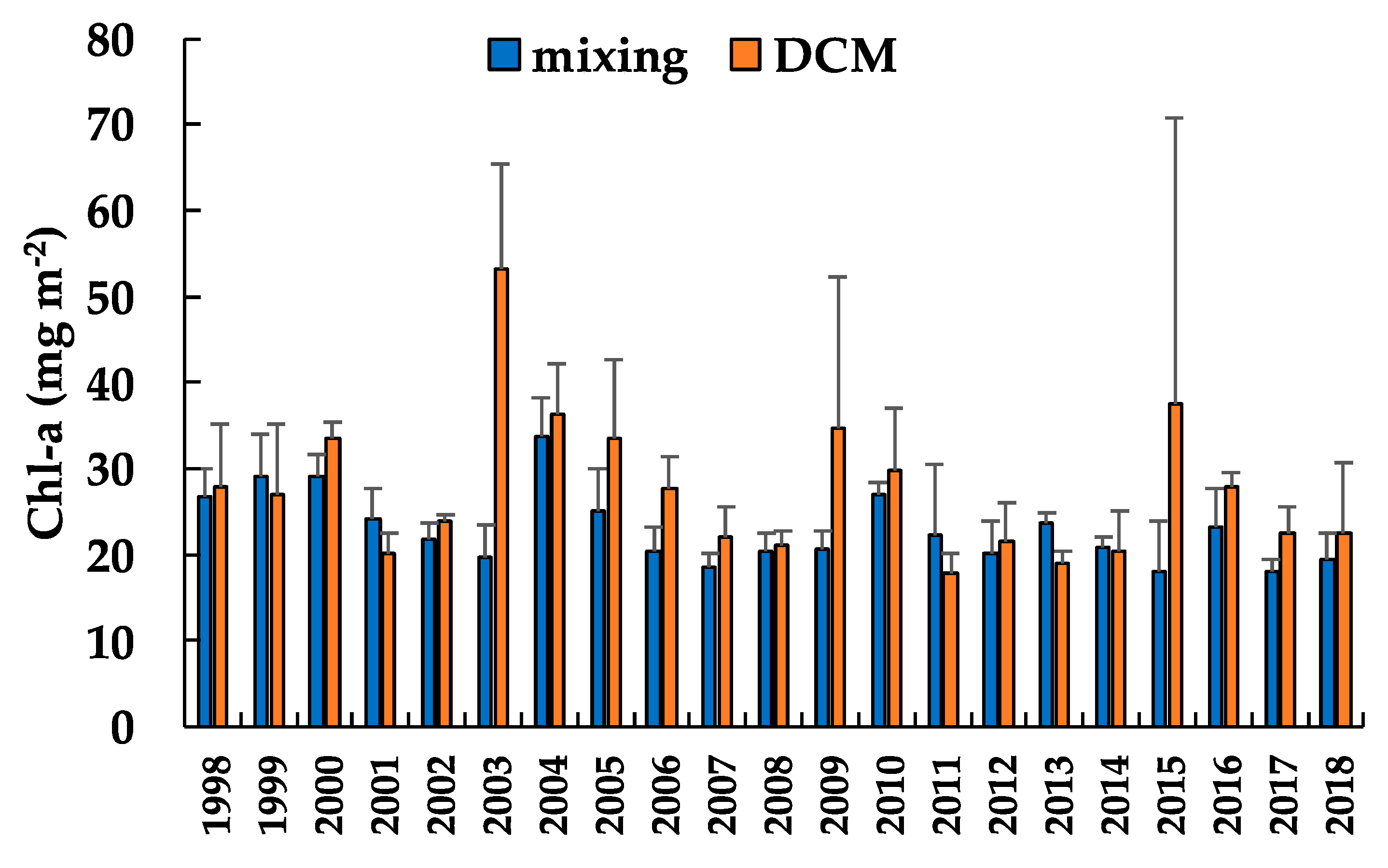
3.1. Chlorophyll-a

We observed substantial variability in the Chl-a concentration in Lake Alchichica throughout 1998–2018 with three extremes (>50 mg m⁻²) peaks: October–November 2003, October 2009, and August–September 2015 (Figure 2). The Chl-a concentration annual average was 23 ± 4 mg m⁻² within 18 ± 4 mg m⁻² and 30 ± 13 mg m⁻². There was a linearly decreasing trend in the Chl-a concentration from 1998 to 2018.

The Chl-a concentration fluctuated interannually (Figure 3). For 48% of the period, the Chl-a concentration was above the annual average, while 52% was below the annual average. The above and below the average Chl-a concentration regularly alternated (three above, two below, three above, three below, two above, four below, two above, two below). Annually, Chl-a concentration displayed a regular dynamic with two peaks (Figure 3). The first peak was associated with the winter (January to March) mixing period when diatoms bloom throughout the water column. The second peak was related to developing a DCM at the metalimnion during the stratification reaching maximum concentrations in September–October.

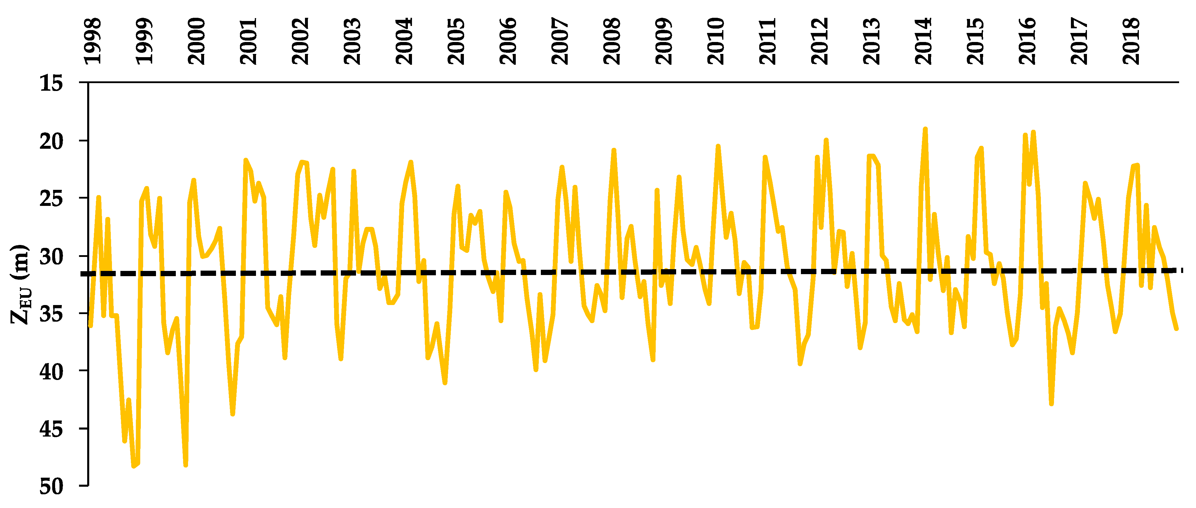
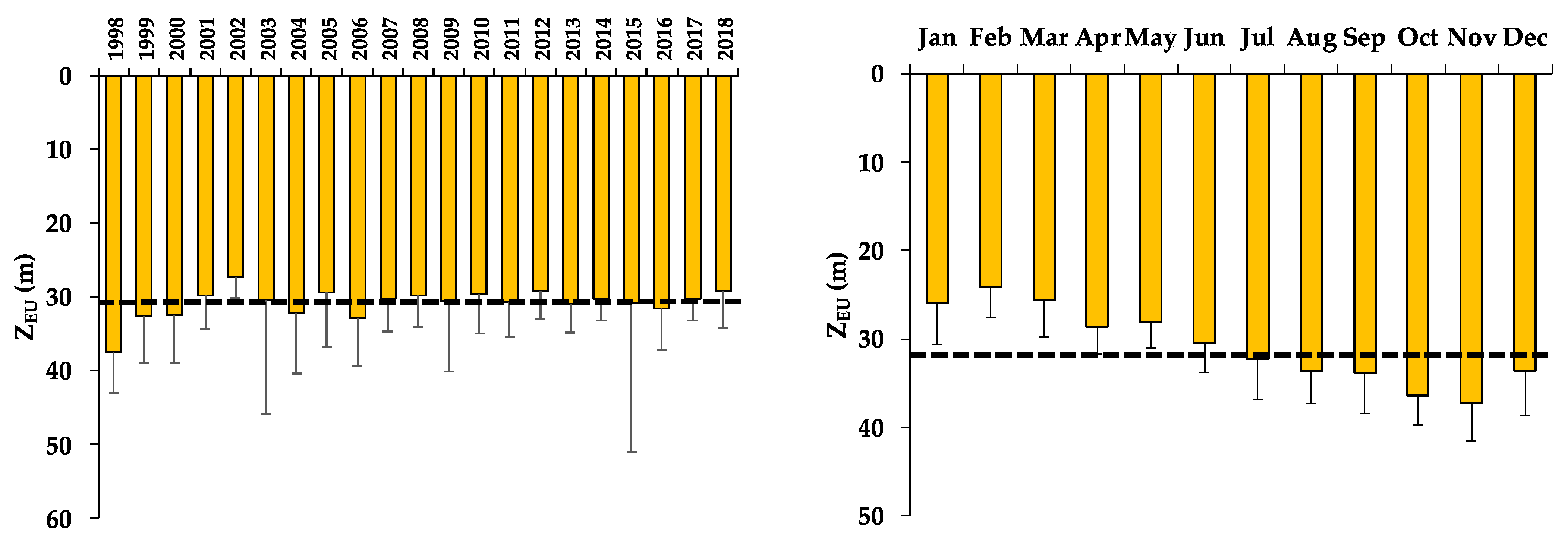
3.2. Euphotic Zone (Z_EU)

There was interannual variability in the euphotic zone (Z_EU) of Lake Alchichica from 1998 to 2018 (Figure 4). A recurrent annual pattern evidences the turbid and the clear water phases. There was a linearly decreasing trend in the Z_EU from 1998 to 2018. The Z_EU annual average was 31 ± 6 m within 27 ± 6 m and 37 ± 8 m.

The Z_EU fluctuated interannually (Figure 5). For 29%, the Z_EU was above the annual average, while for 71%, it was below the annual average. The Z_EU displayed a regular dynamic with two phases annually (Figure 5). The first is the turbid water phase with Z_EU below the annual average (31 m) during the mixing and early stratification (January to June). For the second one, the clear water phase with Z_EU was above the annual average during the well-established and late stratification (July to December).

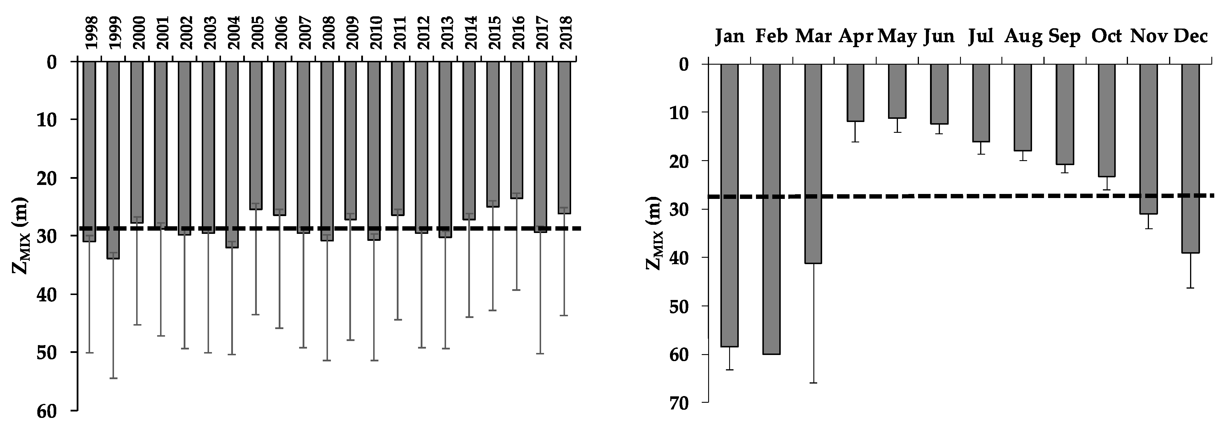
3.3. Mixed Layer Depth (Z_MIX)

The mixed layer depth (Z_MIX) displayed interannual variability in Lake Alchichica from 1998 to 2018 (Figure 6). A recurrent annual pattern evidences the water column mixing and stratification periods. The Z_MIX annual average was 29 ± 10 m within 24 ± 16 m and 34 ± 21 m. There was a linearly decreasing trend in the Z_MIX from 1998 to 2018.

The Z_MIX fluctuated interannually (Figure 7). For 52% of the period, the Z_MIX was above the annual average, while 48% was below the annual average. Annually, the Z_MIX displayed a regular dynamic with two seasons. The first is when Z_MIX is maximum (i.e., the whole water column) during the winter mixing period (January to March). The second one corresponded to the extended stratification season (April to December). The Z_MIX decreased rapidly in April at the onset of the stratification and from then on increased gradually along with the well-established and late stratification. The Z_MIX was above the annual average from January to March and November to December and below the average from April to October (Figure 7).

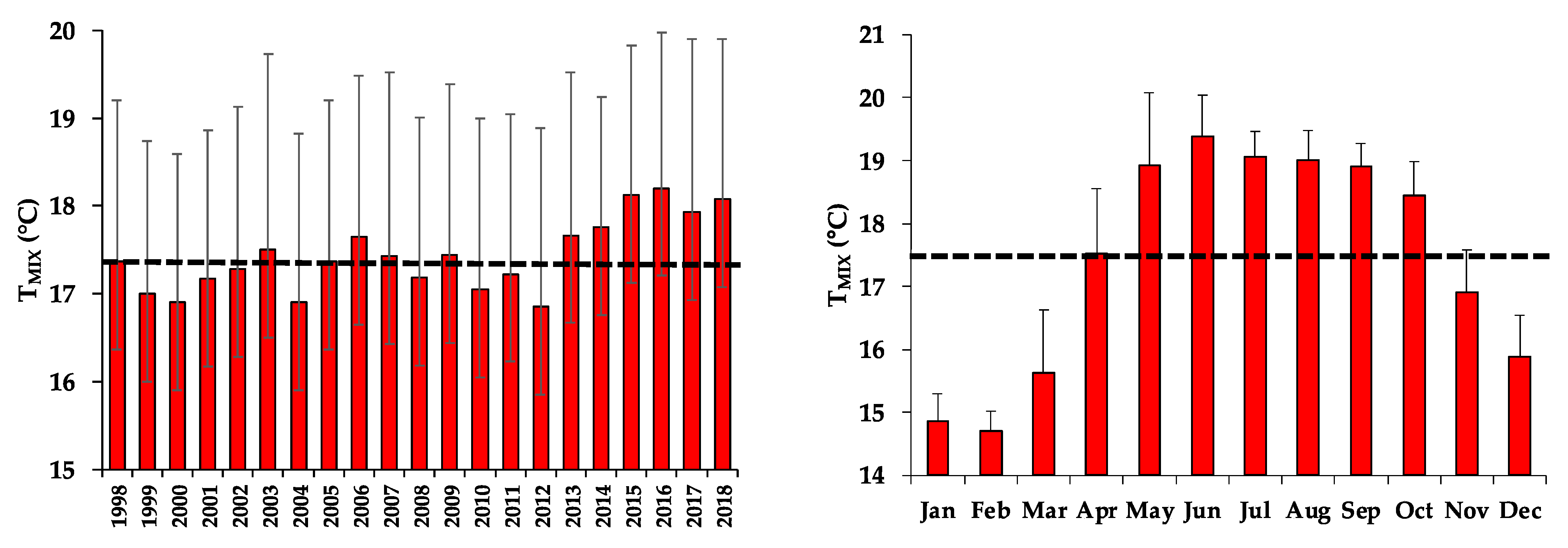
3.4. Temperature of the Mixed Layer (T_MIX)

The mixed layer temperature (T_MIX) displayed interannual variability in Lake Alchichica from 1998 to 2018 (Figure 8). A recurrent annual pattern evidences the cold/dry and the warm/rainy seasons associated with the tropical climate. The T_MIX annual average was 17.4 ± 1.8 °C within a range of 16.9 ± 1.7 °C and 18.2 ± 1.8 °C. There was an increasing linear trend in the T_MIX from 1998 to 2018.

The T_MIX fluctuated interannually (Figure 9). For 48% of the period, the T_MIX was above the annual average, while 52% was below the annual average. The T_MIX displayed a regular dynamic with two periods (Figure 9). The first was when T_MIX was colder (below the average) during the winter and late stratification (January–March, and November–December). The second one corresponded to the well-established and late stratification season (April to October) when T_MIX was warmer (above the average).

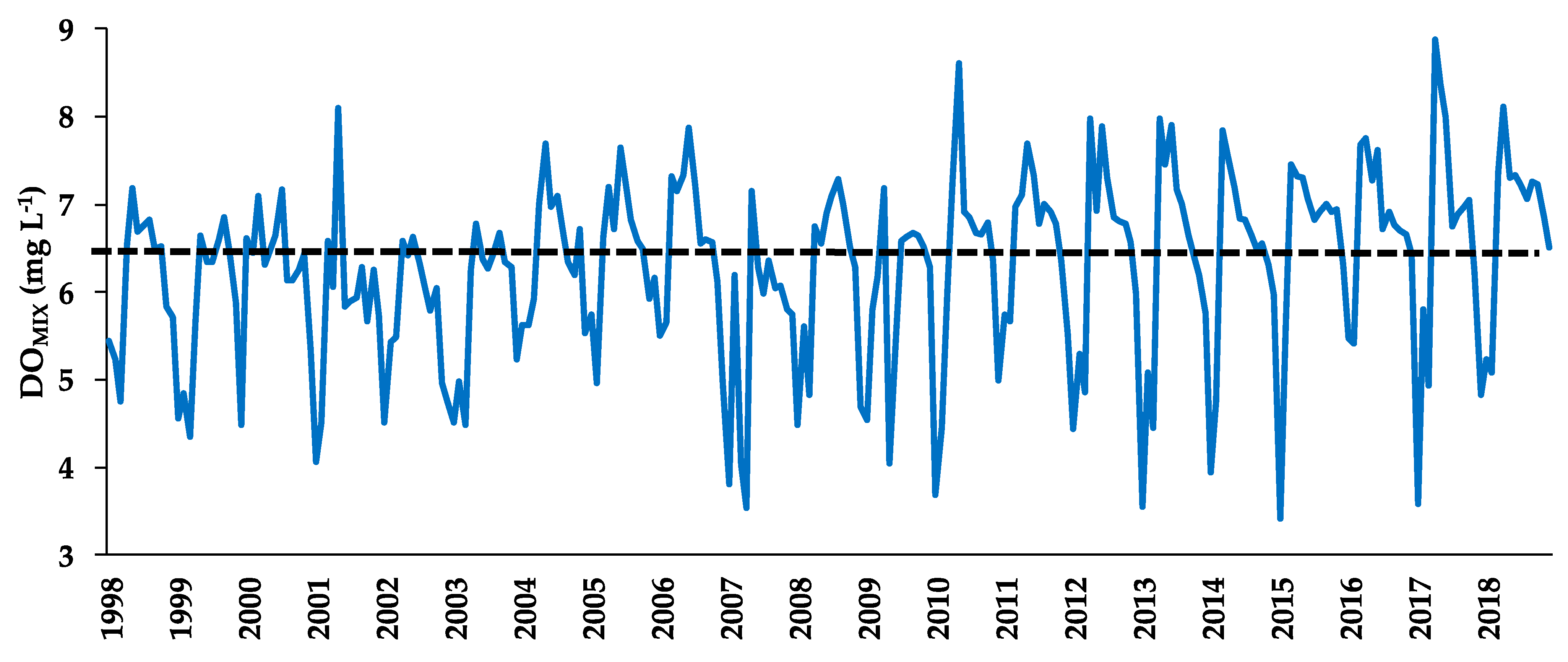
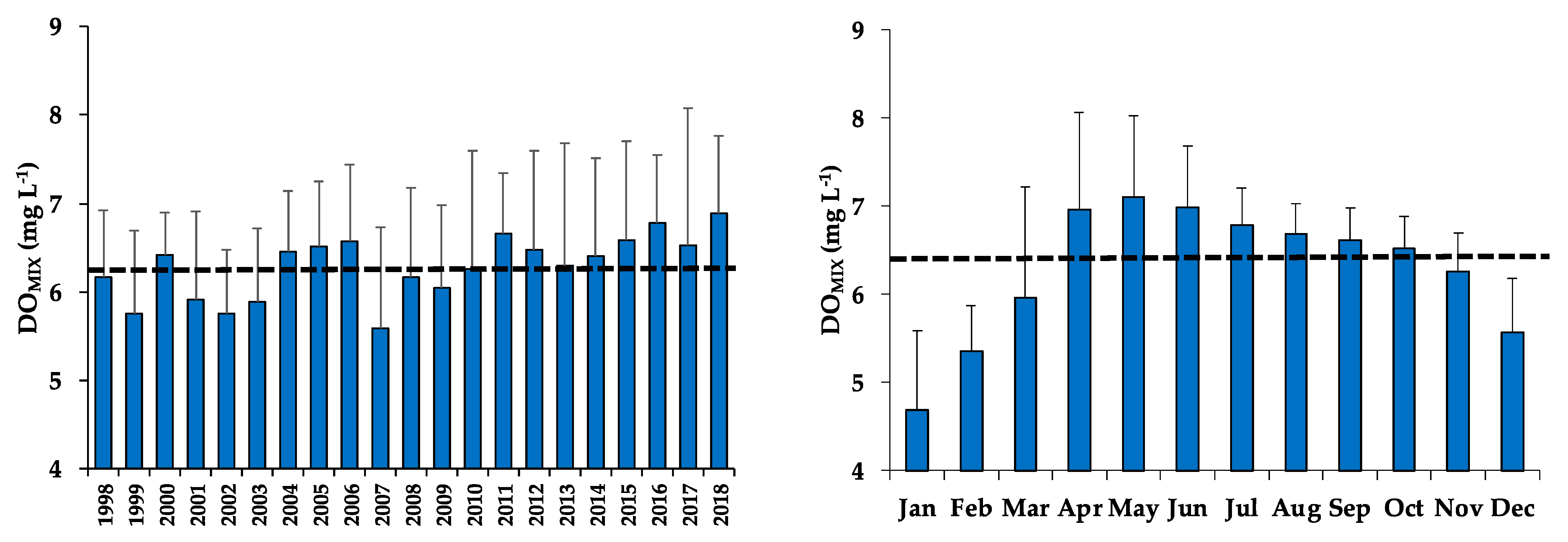
3.5. Dissolved Oxygen of the Mixed Layer (DO_MIX)

The dissolved oxygen concentration of the mixed layer (DO_MIX) displayed interannual variability in Lake Alchichica from 1998 to 2018 (Figure 10). A recurrent annual pattern evidences the water column mixing and stratification periods. The DO_MIX annual average was 6.3 ± 1.0 mg L⁻¹ within 5.6 ± 1.1 mg L⁻¹ and 6.9 ± 0.9 mg L⁻¹. There was an increasing linear trend in the DO_MIX from 1998 to 2018.

The DO_MIX fluctuated interannually (Figure 11). For 57% of the period, the DO_MIX was above the annual average, while 43% was below the annual average. The DO_MIX displayed a regular seasonal dynamic with two periods (Figure 11). The first was when DO_MIX was lower (below the annual average) during the winter and late stratification (January–March and November–December). The second one corresponded to the well-established and late stratification season (April to October) when DO_MIX was higher (above the annual average). The reduction in DO_MIX takes place from the late stratification (through the erosion of the thermocline) to the mixing period when the anoxic hypolimnetic water mixes with the aerobic epilimnetic waters.

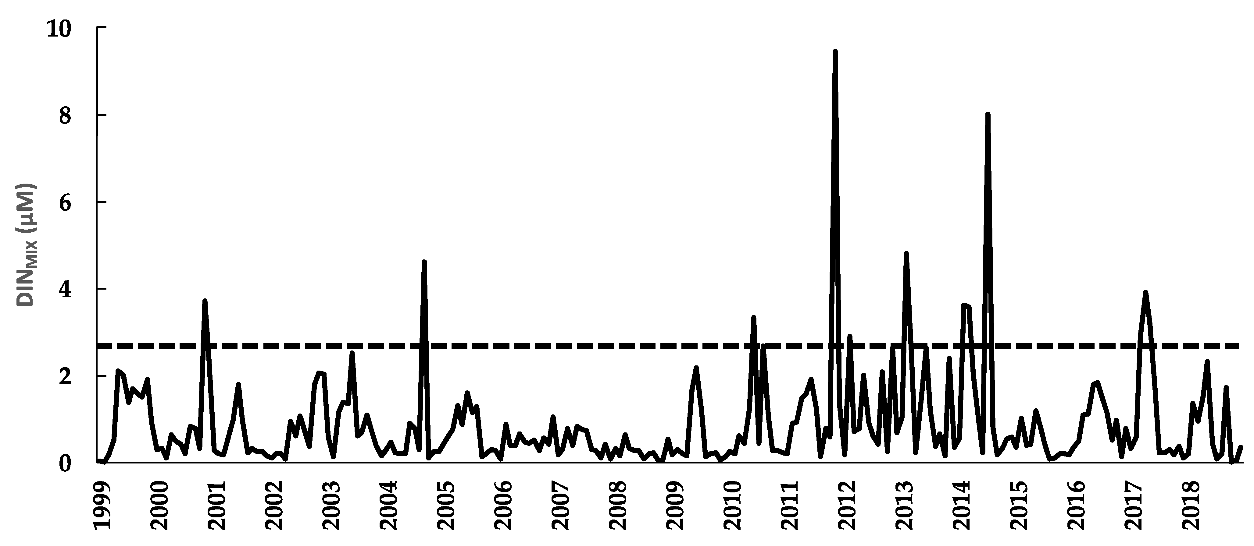
3.6. Dissolved Inorganic Nitrogen of the Mixed Layer (DIN_MIX)

The dissolved inorganic nitrogen concentration in the mixed layer (DIN_MIX) displayed substantial interannual variability in Lake Alchichica from 1999 to 2018 (Figure 12). There was no clear annual pattern of DIN_MIX associated with the water column mixing and stratification periods. The DIN_MIX annual average was 2.7 ± 2.0 µM within a range of 1.1 ± 0.5 µM and 5.1 ± 3.4 µM. There was an increasing linear trend in the DIN_MIX from 1999 to 2018.

The DIN_MIX fluctuated interannually (Figure 13). For 45% of the period, the DIN_MIX was above the annual average, while 55% was below the annual average. The DIN_MIX displayed a regular dynamic with two periods (Figure 13). The first was when DIN was lower (below the annual average) at the onset and along most of the stratification (April, June to October, and December). The second one corresponded primarily to the mixing season (January to March), May, and November, when DIN was higher (above the annual average).

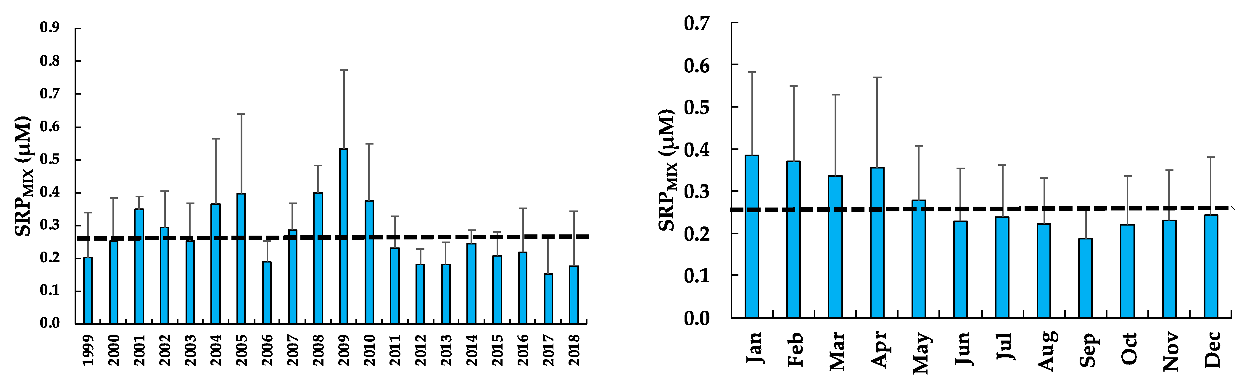
3.7. Soluble Reactive Phosphorus of the Mixed Layer (SRP_MIX)

The soluble reactive phosphorous concentration in the mixed layer (SRP_MIX) displayed substantial interannual variability in Lake Alchichica from 1999 to 2018 (Figure 14). There was no clear annual pattern of the SRP_MIX associated with the water column mixing and stratification periods. The SRP_MIX annual average was 0.27 ± 0.16 µM within a range of 0.15 ± 0.11 µM and 0.53 ± 0.24 µM.

The SRP_MIX fluctuated widely interannually (Figure 15). For 40% of the period, the SRP_MIX was above the annual average, and for 60% was below the annual average. Seasonally, the SRP_MIX displayed a regular dynamic with two periods (Figure 15). The first was when SRP_MIX was lower (below the annual average), and most of the stratification (June to December). The second one corresponded to the mixing season and early stratification (January to May) when SRP_MIX was higher (above the annual average).

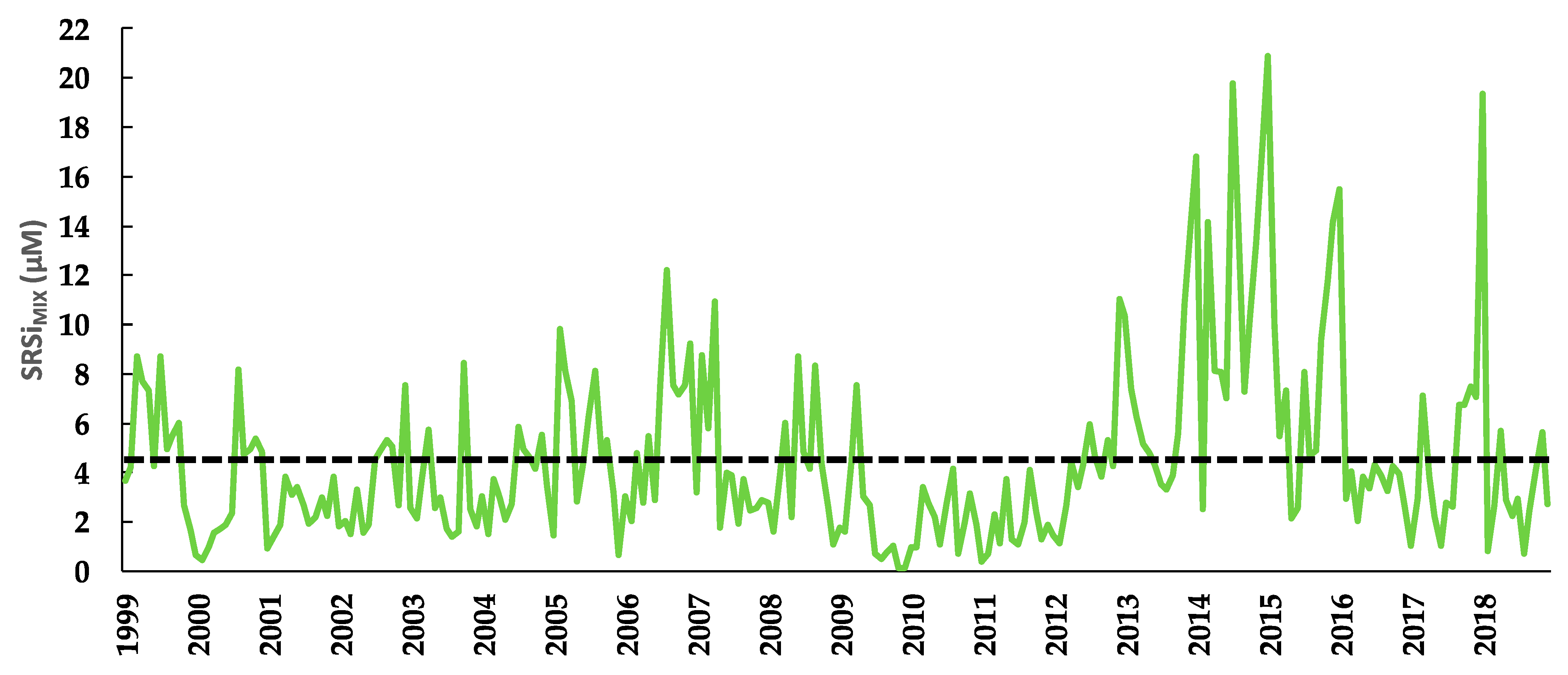
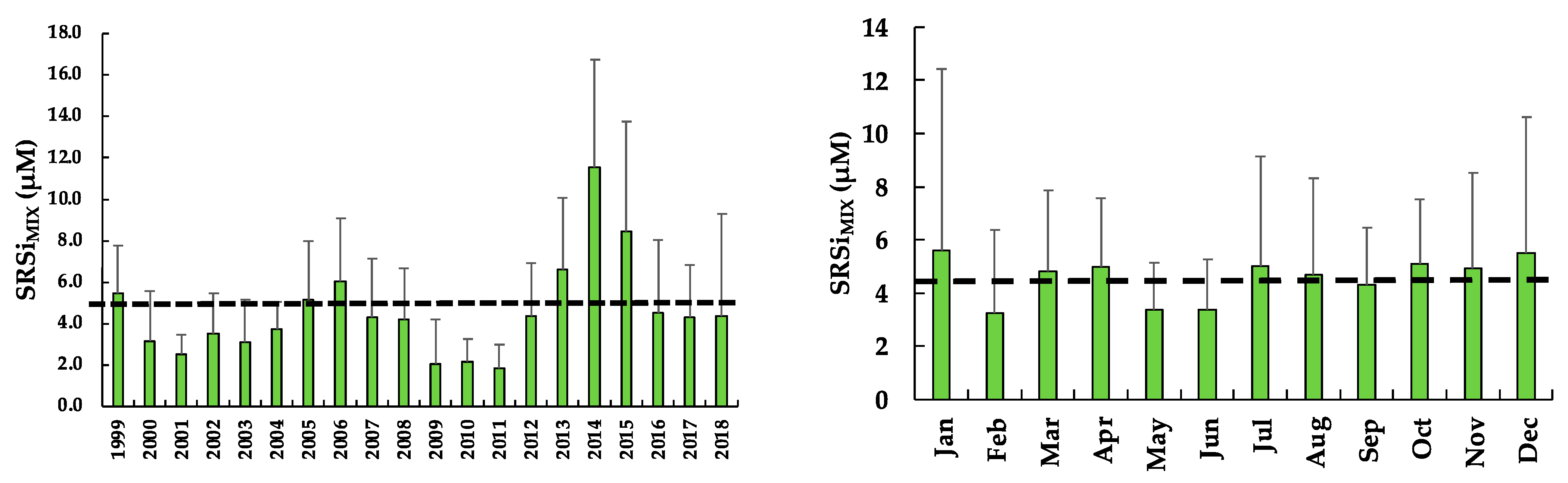
3.8. Soluble Reactive Silica of the Mixed Layer (SRSi_MIX)

The soluble reactive silica concentration in the mixed layer (SRSi_MIX) displayed substantial interannual variability in Lake Alchichica from 1999 to 2018 (Figure 16). There was not a clear annual pattern of the SRSi_MIX associated with the water column mixing and stratification periods. The SRSi_MIX annual average was 4.6 ± 3.6 µM within a range of 1.9 ± 1.1 µM and 11.6 ± 5.2 µM.

The SRSi_MIX fluctuated extensively interannually (Figure 17). For 30% of the period, the SRSi_MIX was above the annual average, and for 70% was below the annual average. The SRSi_MIX displayed irregular dynamic alternating values below and above the annual average (Figure 17). One-third of the year, SRSi_MIX was below the annual average (February, May–June, and September). For the rest of the year (January, March–April, July–August, and October–December), the SRSi_MIX was above the annual average.

3.9. Wavelet Analyses

Wavelet analysis was used to decompose the Chl-a variability from 1998 to 2018 as a function of period and time. We examined if the continuous wavelet transforms could successfully identify variability in the annual scale. The local wavelet power spectrum measures the variance distribution of the time series according to time and periodicity; high variability is represented by red color, whereas blue indicates weak variability. The wavelet spectrum showed that Chl-a (Figure 18) displayed a consistent 1-year periodicity from 1998 until 2012. The strength of the annual periodicity changed over time, suggesting a non-stationary behavior of the time series. There was a weakening of the annual periodicity from 2008 to 2012 until it became statistically non-significant from 2013 to 2015. Moreover, a consistent and statistically significant periodicity between ~4 and 5 years in Chl-a was detected. A semi-annual periodicity was significant for a short time, around 2016, but did not emerge as significant in the global wavelet spectrum. Wavelet analysis of the Multivariate “El Niño Southern Oscillation” (ENSO) Index (MEI) time series (Figure 18) showed a 2-year and a four to five-year periodicity.

However, the former 2-year periodicity showed shifts between 2002 and 2004 and between 2012 and 2015, whereas the latter’s (~4–5 years) period remained stable for the duration of the time series. This shift in periodicity coincides with the shifts in periodicity displayed by the Chl-a wavelet spectrum (Figure 9).Wavelet analysis of the Z_EU, Z_MIX, T_MIX, and DO_MIX showed stable 1-year periodicities for the whole duration of the time series (Figure 19). This steady behavior means that the system’s complexity has not deteriorated so that the seasonality of this process has not perceptibly changed over time. In addition, a 4-year periodicity was significant for the Z_MIX time series.

Finally, the wavelet power spectrum for nutrients (DIN_MIX = dissolved inorganic nitrogen, SRP_MIX = soluble reactive phosphorus, SRSi_MIX = soluble reactive silica) also showed statistically significant periodic structures by the annual (1-year) cycle and, in addition, a 2-year and a ~4–5 years statistically significant periodicities were also characterized for the time series (Figure 20).

All significant scales in the wavelet spectrum were clustered around the 1-year period. However, the power of the annual scale was much lower from 2002 to 2004, except for the SRPMIX time series. Four-year periodicities were statistically significant for most of the nutrient time series. However, the DINMIX time series 2-year periodicity became statistically non-significant after 2005.

4. Discussion

Winder and Cloern [20] found the most common pattern reported in temperate and subtropical aquatic ecosystems, one phytoplankton peak per year or the “canonical spring-bloom pattern” [5,36], to be less frequent than expected (48%), and although the climate-driven annual cycle is an important driver, other factors can mask it leading to other periodicities or even the lack of periodicity [14]. Melack [1] found that most tropical lakes exhibit seasonal fluctuations associated with rainfall, river discharge, or vertical mixing, corresponding to the hydrological (water input-output) or hydrographic (water column and circulation) features of Talling [10]. Lake Alchichica has no river discharge and lies in a semi-desertic area; then, the seasonality is driven by hydrographic features controlled by its thermal stratification and mixing pattern.

Deep tropical lakes are warm-monomictic, showing great regularity in seasonal mixing, which typically coincides with the hemispheric winter (e.g., [37]). Previous studies on Lake Alchichica suggested the latter (e.g., [22,38,39]) and herein confirmed during the 21 annual cycles studied. Lake Alchichica showed a remarkable regularity on the hydrodynamical pattern (warm monomixis), displaying a predictable annual, complete mixing period in winter (January to March) and remained stratified for the remainder of the year. Adame et al. [3] subdivided the stratification period into three stages: (a) early stratification (April to June) when the thermocline was close to the surface and poorly defined, (b) well-established stratification (July to September) when the water column displays a clear layering (epi, meta, and hypolimnion), and (c) late stratification (October to December) when the thermocline deepened and the metalimnion thinned.

The recurrent annual thermal stratification and mixing pattern of Lake Alchichica and its main limnological features could be summarised as follow (

Table 1. Comparison of the main limnological features of Lake Alchichica during the mixing and stratification seasons. (Chl-a: chlorophyll-a concentration, Z_EU: euphotic zone, Z_MIX: mixed layer, T_MIX: temperature in the Z_MIX, OD_MIX: dissolved oxygen concentration in the Z_MIX, DIN_MIX: dissolved inorganic nitrogen in the Z_MIX, SRP_MIX: soluble reactive phosphorous in the Z_MIX, SRSi_MIX: soluble reactive silica in the Z_MIX).

Variable	Mixing (Dry, Cold)	Stratification (Wet, Warm)
Chl-a	High The phytoplankton distributes throughout the water column	High The phytoplankton concentrates at the metalimnion (DCM)
ZEU	Lower Turbid water phase Biogenic turbidity	Higher Clear water phase DCM at the bottom of ZEU
ZMIX	High	Low
TMIX	Colder	Warmer
ODMIX	Lower	Higher
DINMIX	Higher	Lower
SRPMIX	Higher	Lower
SRSiMIX	Higher and lower	Higher and lower

). Z_MIX is at maximum (from surface down to the bottom) during the mixing season, and the water column is cold and well-oxygenated. Nutrients (DIN, SRP, and SRSi) reach high concentrations along the water column, promoting the winter diatom bloom development, resulting in high Chl-a concentration and the lowest values of Z_EU. The mixing season is the turbid water phase associated with high biogenic turbidity. The winter bloom comprises the centric diatom Cyclotella alchichicana [3,26].

At the onset of the stratification period, the warmer and well-lit epilimnion, and nutrient depletion, particularly nitrogen, favored the nitrogen-fixing cyanoprokariota Nodularia aff. spumigena to bloom for a brief period [28]. Monthly, nitrogen was the primary productivity limiting nutrient (DIN_MIX/SRP_MIX < 15, 10 ± 2, 7–14), while interannually, nitrogen was limiting 75% (15 years) and phosphorus 25% (5 years) of the time.

The stratification period corresponds to the clear water phase with high values of Z_EU related to the presence of low Chl-a concentration in the Z_MIX. The Z_MIX remains warm and well-oxygenated. Through the extended stratification season, Z_MIX and Z_EU broaden. While stratified, nutrients are rapidly depleted in the Z_MIX and remain so for the remaining of the stratification, explaining the low Chla concentration in the Z_MIX and the high values of Z_EU.

The large size of C. alchichicana makes it inedible for zooplankton [40,41]. Then most of the diatom bloom is not consumed and incorporated in the food web but instead exported below the thermocline, down to the bottom [42]. A large amount of organic matter deposited into the sediments is partially remineralized by consuming the available dissolved oxygen leading to hypolimnetic anoxia [3], and partially buried and sequestered into the sediments [43]. During the stratification period, the organic matter remineralization explains the nutrient accumulation in the hypolimnion. Along the stratification period, nutrients are depleted in the epilimnion and accumulated in the hypolimnion.

Approximately from September to November, a DCM develops at the metalimnion. The Chl-a concentration at the DCM reaches high values, similar to those recorded in the winter diatom bloom. The DCM is mainly composed of C. alchichicana, which is exported below the thermocline down to the sediments [42]. In this way, two Chl-a peaks are recognized in the annual cycle: a diatom winter blooms along the water column during the mixing season. The second is a DCM at the metalimnion in the stratification.

As previously mentioned, Lake Alchichica showed not one but two phytoplankton peaks per year (Figure 21): the winter bloom (Chl-a: 23 ± 5 mg m⁻²) and the DCM (Chl-a: 28 ± 12 mg m⁻²). The average Chl-a concentration of the mixing period (January to March) was higher than in the DCM in five years (24%), while the Chl-a concentration in the DCM was higher than in the mixing season in sixteen years (76%). The winter diatom bloom duration fluctuated between 1 and 4 months (January–April), with Chl-a concentrations above the 21-year average. January (11, 52.4%) and February (8, 38.1%) were the most representative months of the winter diatom bloom. Differently, in six years (2006–2009 and 2017–2018), the Chl-a concentrations in the diatom bloom were below the average for the whole period. The DCM duration fluctuated between 1 and 5 months (August–December), with Chl-a concentrations above the 21-year average. September and October (14, 66.7%) were the most representative months of the stratification DCM. Contrarily, in two years (2001 and 2011), the Chl-a concentrations in the DCM were below the average for the whole period.

Lewis [44] compared the phytoplankton biomass in temperate and tropical lakes by analyzing the ratio of annual and seasonal mean to maximum biomass. Tropical lakes displayed a higher ratio (0.45) of annual mean to maximum than temperate lakes (0.36). However, the ratio of seasonal mean to maximum biomass (~0.7) was similar in both tropical and temperate lakes. The latter means the intensity of the annual bloom in both tropical and temperate lakes are similar, but tropical lakes display higher minimum Chl-a concentrations throughout the year. The annual ratio of mean to maximum Chl-a in Lake Alchichica ranged between 0.36 and 0.85 (0.68 ± 0.13), which is higher than those reported by Lewis [44] for tropical lakes (0.39 to 0.58) but similar to the seasonal ratio of mean to maximum Chl-a with 0.65 to 0.80. The discrepancy could be that Lewis [44] calculated the seasonal ratio by considering the 3-month interval with the highest biomass, most likely associated with the winter (mixing) bloom. The seasonal ratio of mean to maximum Chl-a calculated for the winter diatom bloom (3 months, January to March) in Lake Alchichica is 0.62, slightly lower than the seasonal ratio of Lewis [44] with 0.65 to 0.80.

The seasonal ratio of mean to maximum Chl-a calculated for the DCM (4 months, August to November) is 0.36, much lower than the seasonal ratio of Lewis [44] with 0.65 to 0.80. The three largest Chl-a concentration peaks could have biased this low value throughout 21 years, corresponding to the DCM (October 2003, October 2009, September 2015).

The annual variation in phytoplankton biomass in temperate lakes is greater than in tropical lakes [44]. Kalff and Watson [45] found that Lake Naivasha had low and seasonal variable (10×) phytoplankton biomass. Differently, the coefficient of variation in Lake Alchichica annual phytoplankton biomass averages 27 ± 14%, and low (1.3×) seasonal variation in biomass (i.e., mixing: 23 ± 5 mg m⁻², early stratification: 19 ± 4 mg m⁻², well-established stratification: 25 ± 10 mg m⁻², and late stratification: 25 ± 10 mg m⁻²). There were also interannual differences in the max:min biomass ratio with an average of 2.4 ± 1.0 (1.5 to 6.1). The inter-annual variability of Chl-a was high -.7×- (annual mean: 18 to 30 mg m⁻²), similarly to Lake Kivu with 1.9× [12].

Our analyses showed that continuous wavelet transforms successfully detect the phenology of the Chl-a concentration and associated limnological parameters over time. Throughout the time series, periodicities associated with the annual cycle represented the dominant scale of variation. As mentioned, the recurrent and predictable annual cyclicity is explained mainly by the warm-monomictic thermal pattern of Lake Alchichica, with the water column mixing being the most important driving force explaining the seasonality.

However, the Chl-a continuous wavelet transforms identified a temporary decrease in the strength of the annual periodicity. While the annual periodicity was the most important scale of variation for the Chl-a during 1998–2010, it was significantly weakened from 2011 to 2015, when it became no longer statistically significant. In this period, there were slight decreases (Z_EU, Z_MIX) and increases (T_MIX, DO_MIX) in the limnological variables associated with decreases in Chl-a concentration. Interestingly, this shift in periodicity in the Chl-a power spectrum between 2011 and 2015 coincided with intense La Niña events (2011–2012) and with the “Godzilla” El Niño event (2015).

Tropical lakes are particularly sensitive to climate change [46,47]. A previous study [40]) reported that the 1998–1999 El Niño resulted in higher epilimnetic temperatures and lower Chl-a concentrations in Lake Alchichica. Recently, Alcocer et al. [40] found that the air temperature in the Lake Alchichica region increased from 1966 to 2018. This variability was correlated positively with the Oceanic Niño Index (ONI), the Pacific Decadal Oscillation index (PDO), and the Atlantic Multidecadal Oscillation index (AMO), and negatively with the Southern Oscillation Index (SOI). T_MIX temperature displayed an increasing trend associated with the air temperature increase, while Chl-a concentration displayed a decreasing trend (

Table 2. Mann–Kendall test results for trend analyses of phytoplanktonic chlorophyll-a concentration (1998–2018), water quality (1998–2018), and trophic (1999–2018) variables of Lake Alchichica. (Chl-a: chlorophyll-a concentration, Z_EU: euphotic zone, Z_MIX: mixed layer, T_MIX: temperature in the Z_MIX, OD_MIX: dissolved oxygen concentration in the Z_MIX, DIN_MIX: dissolved inorganic nitrogen in the Z_MIX, SRP_MIX: soluble reactive phosphorous in the Z_MIX, SRSi_MIX: soluble reactive silica in the Z_MIX).

Variable	S	Z	P	Trend
Chl-a	−4045	−3.4669	0.00052653	Decreasing
ZEU	−1397	−1.0255	0.30513	Non-Significant
ZMIX	−1977	−1.4539	0.14599	Non-Significant
TMIX	4341	3.1881	0.001432	Increasing
ODMIX	6063	4.4531	8.4643 × 10−6	Increasing
DINMIX	−5525	−4.4426	8.8884 × 10−6	Decreasing
SRPMIX	−5570	−4.4796	7.4786 × 10−6	Decreasing
SRSiMIX	2751	2.212	0.026964	Increasing

). Higher temperatures associated with climate change resulted in stronger thermal stratifications, lower Z_MIX, and lower nutrient concentration availability. DIN_MIX and SRP_MIX displayed decreasing trends; contradictorily, SRSi_MIX showed an increasing trend related to the decreasing trend in Chl-a, indicating lower biomass of diatoms and consequently less SRSi uptake.

Regarding the 2-year and 4-year periodicities revealed through the continuous wavelet transforms analyses, the biennial cycle in the Chl-a concentration was already reported in Adame et al. [3]. Adame et al. [3] reported higher Chl-a concentrations during the winter diatom blooms of even years while lower in odd years. Higher silicate concentration and Si/N ratio in the hypolimnion during the previous late stratification period led to higher diatom blooms in the following mixing period. Herein, we confirmed the biennial (2-year) cyclicity and provided a plausible explanation of the role silicate and the Si/N ratio play in controlling the phytoplankton biomass in Lake Alchichica.

As mentioned before, the large size of C. alchichicana makes it inedible for zooplankton. Then most of the biomass is exported below the thermocline down to the sediments [27]. C. alchichicana contributes 98% to the silica flux down to the sediments in Lake Alchichica with 147 g m⁻² year⁻¹ [42]. Oseguera et al. [48] found the particles captured in sediment traps deployed in Lake Alchichica evaluating exportation into the deep sediments were biogenic, primarily composed of cells of C. alchichicana.

Alcocer et al. [43] found high preservation of biogenic carbon—and associated diatom silica—in the deep sediments of Lake Alchichica, suggesting a net carbon and silica lost out of the system. Lake Alchichica, with a low silica concentration availability and phytoplankton biomass dominated by large diatoms, deep, thorough mixing events are crucial for silica mineralization and recycling instead of sequestering. Mineralization and mixing events also replenish the lake with nitrogen which often limits phytoplankton in tropical lakes [49], as in Lake Alchichica [25,50], confirmed by the recurrent annual bloom of N. aff. spumigena [28], a nitrogen-fixing cyanobacteria [51].

Climate variability leads to warmer temperatures, which increase the length and strength of thermal stratification (e.g., [52]), preventing nutrient mineralization and recycling. Opposite, colder temperatures favor complete water column mixing and re-oxygenation, favoring nutrient mineralization and recycling, which brought an increased supply of phosphorus and, more importantly, nitrogen which later controlled phytoplankton growth in the Z_EU.

Moreover, there was a ~4–5 years periodicity evidenced in nutrient concentration. We think these 2-year and ~4–5 years periodicities could be associated with ENSO events encompassing stronger winds and then more profound, more complete mixing seasons providing higher nutrient concentrations stimulating larger blooms as suggested by Alcocer et al. [40].

5. Conclusions

This work confirmed that wavelet analysis could help us interpret multi-scale, non-stationary time-series data to reveal features that could not otherwise be seen. By using a long-term (1998–2018) limnological database of the tropical, saline Lake Alchichica, we (a) verified the regularity of the annual cycle of the phytoplankton Chl-a associated with the warm-monomictic thermal-mixing-pattern, (b) revealed the phenology of the annual Chl-a cycle showing large inter-annual variability, (c) identified the presence of a biennial cycle most likely controlled through SRSi availability and Si/N ratio associated to climate variability influencing the length and strength of the annual thermal stratification, and (d) recognize other cycles with different periodicities associated with external forcing agents (e.g., ENSO-El Niño Southern Oscillation). The water quality variables were regular along the 21 years, displaying a recurrent annual pattern. Nutrient concentration, as trophic indicators, revealed the same cyclicity (1-year, 2-year, and ~4–5 years) as Chl-a, suggesting the external forcing agents lead to deeper, more complete mixing events increasing nutrient availability, which in turn stimulate larger Chl-a concentrations.

References

- Melack, J.M. Primary productivity and fish yields in tropical lakes. Trans. Am. Fish. Soc. 1976, 105, 575–580. [Google Scholar] [CrossRef]
- Field, C.B.; Behrenfeld, M.J.; Randerson, J.T.; Falkowski, P. Primary production of the biosphere: Integrating terrestrial and oceanic components. Science 1998, 281, 237–242. [Google Scholar] [CrossRef] [Green Version]
- Adame, M.F.; Alcocer, J.; Escobar, E. Size-fractionated phytoplankton biomass and its implications for the dynamics of an oligotrophic tropical lake. Freshw. Biol. 2008, 53, 22–31. [Google Scholar] [CrossRef]
- Talling, J.F.; Lemoalle, J. Ecological Dynamics of Tropical Inland Waters; Cambridge University Press: Cambridge, UK, 1998; p. 452. [Google Scholar]
- Sommer, U.; Gliwicz, Z.M.; Lampert, W.; Duncan, A. The PEG-model of seasonal succession of planktonic events in freshwaters. Arch. Für Hydrobiol. 1986, 106, 433–471. [Google Scholar]
- Sommer, U.; Adrian, R.; De Senerpont Domis, L.; Elser, J.J.; Gaedke, U.; Ibelings, B.; Jeppesen, E.; Lürling, M.; Molinero, J.C.; Mooij, W.M.; et al. Beyond the Plankton Ecology Group (PEG) model: Mechanisms driving plankton succession. Annu. Rev. Ecol. Evol. Syst. 2012, 43, 429–448. [Google Scholar] [CrossRef]
- Carey, C.C.; Hanson, P.C.; Lathrop, R.C.; St. Amand, A.L. Using wavelet analyses to examine variability in phytoplankton seasonal succession and annual periodicity. J. Plankton Res. 2016, 38, 27–40. [Google Scholar] [CrossRef] [Green Version]
- Sarmento, H. New paradigms in tropical limnology: The importance of the microbial food web. Hydrobiologia 2012, 686, 1–14. [Google Scholar] [CrossRef]
- Plisnier, P.D.; Nshombo, M.; Mgana, H.; Ntakimazi, G. Monitoring climate change and anthropogenic pressure at Lake Tanganyika. J. Great Lakes Res. 2018, 44, 1194–1208. [Google Scholar] [CrossRef]
- Talling, J.F. The seasonality of phytoplankton in African lakes. Hydrobiologia 1986, 138, 138–160. [Google Scholar] [CrossRef]
- Lewis, W.M.J. Phytoplankton succession in Lake Valencia, Venezuela. Hydrobiologia 1986, 138, 189–203. [Google Scholar] [CrossRef]
- Darchambeau, F.; Sarmento, H.; Descy, J.-P. Primary production in a tropical large lake: The role of phytoplankton composition. Sci. Total Environ. 2014, 473–474, 178–188. [Google Scholar] [CrossRef]
- Kilham, P.; Kilham, S.S. Endless summer: Internal loading processes dominate nutrient cycling in tropical lakes. Freswater Biol. 1990, 23, 379–389. [Google Scholar] [CrossRef]
- Rugema, E.; Darchambeau, F.; Sarmento, H.; Stoyneva-Gärtner, M.; Leitao, M.; Thiery, W.; Latli, A.; Descy, J.P. Long-term change of phytoplankton in Lake Kivu: The rise of the greens. Freshw. Biol. 2019, 64, 1940–1955. [Google Scholar] [CrossRef]
- Cloern, J.E.; Jassby, A.D. Complex seasonal patterns of primary producers at the land–sea interface. Ecol. Lett. 2008, 11, 1294–1303. [Google Scholar] [CrossRef]
- Paerl, H.W.; Huisman, J. Blooms like it hot. Science 2008, 320, 57–58. [Google Scholar] [CrossRef] [Green Version]
- Garcia-Soto, C.; Pingree, R.D. Spring and summer blooms of phytoplankton (SeaWiFS/MODIS) along a ferry line in the Bay of Biscay and western English Channel. Cont. Shelf Res. 2009, 29, 111–1122. [Google Scholar] [CrossRef]
- Cloern, J.E.; Jassby, A.D. Patterns and scales of phytoplankton variability in estuarine–coastal ecosystems. Estuaries Coasts 2010, 33, 230–241. [Google Scholar] [CrossRef] [Green Version]
- Smayda, T.J. Patterns of variability characterizing marine phytoplankton, with examples from Narragansett Bay. ICES J. Mar. Sci. 1998, 55, 562–573. [Google Scholar] [CrossRef] [Green Version]
- Winder, M.; Cloern, J.E. The annual cycles of phytoplankton biomass. Philos. Trans. R. Soc. B 2010, 365, 230–241. [Google Scholar] [CrossRef]
- Mallat, S. A Wavelet Tout of Signal Processing; Academic Press: San Diego, CA, USA, 1998; p. 832. [Google Scholar]
- Alcocer, J.; Lugo, A.; Escobar, E.; Sánchez, M.R.; Vilaclara, G. Water column stratification and its implications in the tropical warm monomictic Lake Alchichica, Puebla, Mexico. Verh. des Int. Ver. Limnol. 2000, 27, 3166–3169. [Google Scholar] [CrossRef]
- Filonov, A.; Tereshchenko, I.; Barba-Lopez, M.R.; Alcocer, J.; Ladah, L. Meteorological regime, local climate, and hydrodynamics of Lake Alchichica. In Lake Alchichica Limnology—The Uniqueness of a Tropical Maar Lake; Alcocer, J., Ed.; Springer: Cham, Switzerland, 2022; pp. 75–99. [Google Scholar]
- Silva-Aguilera, R.A.; Vilaclara, G.; Armienta, M.A.; Escolero, O. Hydrogeology and hydrochemistry of the Serdán-Oriental basin and the Lake Alchichica. In Lake Alchichica Limnology—The Uniqueness of a Tropical Maar Lake; Alcocer, J., Ed.; Springer: Cham, Switzerland, 2022. [Google Scholar]
- Ramírez-Olvera, M.A.; Alcocer, J.; Merino-Ibarra, M.; Lugo, A. Nutrient limitation in a tropical saline lake: A microcosm experiment. Hydrobiologia 2009, 626, 5–13. [Google Scholar] [CrossRef]
- Oliva, M.G.; Lugo, A.; Alcocer, J.; Peralta, L.; Sánchez, M.R. Phytoplankton dynamics in a deep, tropical, hyposaline lake. Hydrobiologia 2001, 446, 299–306. [Google Scholar] [CrossRef]
- Vilaclara, G.; Oliva-Martínez, M.G.; Macek, M.; Ortega-Mayagoitia, E.; Alcántara-Hernández, R.J.; López-Vázquez, C. Phytoplankton of Alchichica: A unique community for an oligotrophic lake. In Lake Alchichica Limnology—The Uniqueness of a Tropical Maar Lake; Alcocer, J., Ed.; Springer: Cham, Switzerland, 2022; pp. 192–211. [Google Scholar]
- Oliva, M.G.; Lugo, A.; Alcocer, J.; Peralta, L.; Oseguera, L.A. Planktonic bloom-forming Nodularia in the saline Lake Alchichica, Mexico. In Saline Lakes Around the World: Unique Systems with Unique Values; Oren, A., Naftz, D.L., Wurtsbaugh, W.A., Eds.; The S.J. and Jessie E. Quinney Natural Resources Research Library, College Of Natural Resources, Utah State University: Logan, UT, USA, 2009; pp. 121–126. [Google Scholar]
- Keifer, D.A.; Chamberlain, W.S.; Booth, C.R. Natural fluorescence of chlorophyll a: Relationship to photosynthesis and chlorophyll concentration in the western South Pacific gyre. Limnol. Oceanogr. 1989, 34, 868–881. [Google Scholar] [CrossRef]
- Chamberlain, W.S.; Booth, C.R.; Keifer, D.A.; Morrow, J.H.; Murphy, R.C. Evidence for a simple relationship between natural fluorescence, photosynthesis and chlorophyll in the sea. Deep-Sea Res. 1990, 37, 951–973. [Google Scholar] [CrossRef]
- Hansen, H.P.; Koroleff, F. Determination of nutrients. In Methods of Seawater Analysis; Grasshoff, K., Kremling, K., Ehrhardt, M., Eds.; Wiley-Verlag: Weinheim, Germany, 1999; pp. 159–228. [Google Scholar]
- R Development Core Team. R: A Language and Environment for Statistical Computing; R Foundation for Statistical Computing: Vienna, Austria, 2020; Available online: https://www.R-project.org/ (accessed on 6 August 2021).
- Percival, D.B.; Walden, A.T. Wavelet Methods for Time Series Analysis; Cambridge University Press: Cambridge, UK, 2000. [Google Scholar]
- Ruffinatti, F.A.; Lovisolo, D.; Distasi, C.; Ariano, P.; Erriquez, J.; Ferraro, M. Calcium signals: Analysis in time and frequency domains. J. Neurosci. Methods 2011, 199, 310–320. [Google Scholar] [CrossRef]
- Torrence, C.; Compo, G.P. A practical guide to wavelet analysis. Bull. Am. Meteorol. Soc. 1998, 79, 61–78. [Google Scholar] [CrossRef] [Green Version]
- Cushing, D.H. The seasonal variation in oceanic production as a problem in population dynamics. ICES J. Mar. Sci. 1959, 24, 455–464. [Google Scholar] [CrossRef]
- Lewis, W.M., Jr. Tropical lakes: How latitude makes a difference. In Perspectives in Tropical Limnology; Schiemer, F., Boland, K.T., Eds.; SPB Academic Publishing: Amsterdam, The Netherlands, 1996; pp. 43–64. [Google Scholar]
- Cuevas-Lara, J.D.; Alcocer, J.; Oseguera, L.A.; Quiroz-Martínez, B. Dinámica Largo Plazo (1999–2014) de la Productividad Primaria Fitoplanctónica en el Lago Alchichica, Puebla. In Estado Actual del Conocimiento del Ciclo del Carbono y sus Interacciones en México: Síntesis a 2016; Paz Pellat, F., Wong González, J., Torres Alamilla, R., Eds.; Serie Síntesis Nacionales; Programa Mexicano del Carbono en colaboración con la Universidad Autónoma del Estado de Hidalgo: Texcoco, México, 2016; p. 732. [Google Scholar]
- González Contreras, C.G.; Alcocer, J.; Oseguera, L.A. Clorofila a fitoplanctónica en el lago tropical profundo Alchichica: Un registro de largo plazo (1999–2010). Hidrobiológica 2015, 25, 347–356. [Google Scholar]
- Alcocer, J.; Lugo, A.; Fernández, R.; Vilaclara, G.; Oliva, M.G.; Oseguera, L.A.; Silva-Aguilera, R.A.; Escolero, Ó. 20 years of global change on the limnology and plankton of a tropical, high-altitude lake. Diversity 2022, 14, 190. [Google Scholar] [CrossRef]
- Fernández, R.; Alcocer, J.; Lugo, A.; Oseguera, L.A.; Guadarrama-Hernández, S. Seasonal and interannual dynamics of pelagic rotifers in a tropical, saline, deep lake. Diversity 2022, 14, 113. [Google Scholar] [CrossRef]
- Ardiles, V.; Alcocer, J.; Vilaclara, G.; Oseguera, L.A.; Velasco, L. Diatom fluxes in a tropical, oligotrophic lake dominated by large-sized phytoplankton. Hydrobiologia 2012, 679, 77–90. [Google Scholar] [CrossRef]
- Alcocer, J.; Ruíz-Fernández, R.; Escobar, E.; Pérez-Bernal, L.H.; Oseguera, L.A.; Ardiles-Gloria, V. Deposition, burial and sequestration of carbon in an oligotrophic, tropical lake. J. Limnol. 2014, 72, 223–235. [Google Scholar] [CrossRef] [Green Version]
- Lewis, W.M., Jr. Comparisons of phytoplankton biomass in temperate and tropical lakes. Limnol. Oceanogr. 1990, 35, 1838–1845. [Google Scholar] [CrossRef] [Green Version]
- Kalff, J.; Watson, S. Phytoplankton and its dynamics in two tropical lakes: A tropical and temperate zone comparison. Hydrobiologia 1986, 138, 161–176. [Google Scholar] [CrossRef]
- Descy, J.P.; Sarmento, H. Microorganisms of the East African Great Lakes and their response to environmental changes. Freshw. Rev. 2008, 1, 59–73. [Google Scholar] [CrossRef] [Green Version]
- Kraemer, B.M.; Pilla, R.M.; Woolway, R.I.; Anneville, O.; Ban, S.; Colom-Montero, W.; Devlin, S.P.; Dokulil, M.T.; Gaiser, E.E.; Hambright, K.D.; et al. Climate change drives widespread shifts in lake thermal habitat. Nat. Clim. Change 2021, 11, 521–529. [Google Scholar] [CrossRef]
- Oseguera, L.A.; Alcocer, J.; Vilaclara, G. Relative importance of dust inputs and aquatic biological production as sources of lake sediments in an oligotrophic lake in a semi-arid area. Earth Surf. Process. Landf. 2011, 3, 419–426. [Google Scholar] [CrossRef]
- Lewis, W.M., Jr. Causes for the high frequency of nitrogen limitation in tropical lakes. Verh. des Int. Ver. Limnol. 2002, 28, 210–213. [Google Scholar] [CrossRef]
- Ramos-Higuera, E.; Alcocer, J.; Ortega-Mayagoitia, E.; Camacho, A. Nitrógeno: Elemento limitante para el crecimiento fitoplanctónico en un lago oligotrófico tropical. Hidrobiológica 2008, 18, 105–113. [Google Scholar]
- Falcón, L.I.; Escobar-Briones, E.; Romero, D. Nitrogen fixation patterns displayed by cyanobacterial consortia in Alchichica crater-lake, Mexico. Hydrobiologia 2002, 467, 71–78. [Google Scholar] [CrossRef]
- Butcher, J.B.; Nover, D.; Johnson, T.E.; Clark, C.M. Sensitivity of lake thermal and mixing dynamics to climate change. Clim. Chang. 2015, 129, 295–305. [Google Scholar] [CrossRef] [Green Version]