
Buffalo Pound Lake—Modelling Water Resource Management Scenarios of a Large Multi-Purpose Prairie Reservoir


1
Global Institute for Water Security, School of Environment and Sustainability, University of Saskatchewan, Saskatoon, SK S7N 3H5, Canada
2
Water Security Agency, 10-3904 Millar Avenue, Saskatoon, SK S7P 0B1, Canada
3
School of Environment and Sustainability, University of Saskatchewan, Saskatoon, SK S7N 5C8, Canada
*
Author to whom correspondence should be addressed.
Water 2022, 14(4), 584; https://doi.org/10.3390/w14040584
Submission received: 18 January 2022
/
Revised: 8 February 2022
/
Accepted: 10 February 2022
/
Published: 15 February 2022
(This article belongs to the Special Issue Surface Water Quality Modelling)
Abstract
:Water quality models are an emerging tool in water management to understand and inform decisions related to eutrophication. This study tested flow scenario effects on the water quality of Buffalo Pound Lake—a eutrophic reservoir supplying water for approximately 25% of Saskatchewan’s population. The model CE-QUAL-W2 was applied to assess the impact of inter-basin water diversion after the impounded lake received high inflows from local runoff. Three water diversion scenarios were tested: continuous flow, immediate release after nutrient loading increased, and a timed release initiated when water levels returned to normal operating range. Each scenario was tested at three different transfer flow rates. The transfers had a dilution effect but did not affect the timing of the nutrient peaks in the upstream portion of the lake. In the lake’s downstream section, nutrients peaked at similar concentrations as the base model, but peaks arrived earlier in the season and attenuated rapidly. Results showed greater variation among scenarios in wet years compared to dry years. Dependent on the timing and quantity of water transferred, some but not all water quality parameters are predicted to improve along with the water diversion flows over the period tested. The results suggest that it is optimal to transfer water while local watershed runoff is minimal.
1. Introduction
A variety of management tools are required to effectively understand, predict, and optimize surface water quality. This includes traditional information such as data from well-designed monitoring programs, and increasingly relies on the use of water quality models. Water quality models are critical for assessing situations that cannot be directly measured, to better understand system constrains, and for examining scenarios, including operational changes. Reservoir management has benefitted especially from the growing application of water quality models to the problems of regulated flowthrough and anthropogenic water demands. These models have been applied globally to issues such as selective withdrawal strategies for optimizing water temperatures and quality e.g., [1,2,3,4], and water quality simulations e.g., [5,6,7]. Other uses include modelling nutrient loading from the watershed [8,9], impacts of pisciculture [10], reservoir contaminant scenarios [11], and impacts of changing climate and streamflow on reservoir water quality [12].
Canada has one of the highest rates of water availability per capita per year [13]. Canada also has one of the world’s highest per capita water use [14]. The Prairie region contains 80% of Canada’s agriculture [15], with agriculture accounting for an 86.5% share of surface water use in the South Saskatchewan River Basin [16]. The climate of the Prairies is highly variable with an extreme temperature range and periodic floods and droughts [15]. The landscape is semi-arid, and many users compete for limited water resources [17]. Population growth and irrigation expansion will place further pressure on Prairie reservoirs showing signs of water stress [18].
Buffalo Pound Lake
Buffalo Pound Lake (BPL) is the water source for approximately 25% of the provincial population of Saskatchewan, Canada. Water demands from BPL include municipal, industrial, and agricultural abstractions, and the lake is an important recreational waterbody. The importance of BPL has resulted in numerous scientific studies over the years e.g., [19,20,21,22,23,24], and organizational reports from environmental consultancy firms and government agencies. The water quality of BPL is a continuing concern. The lake is situated in an area that experiences high runoff variability associated with its variable climate and is therefore subject to periods of both high and low runoff. BPL is located within a former glacial-melt channel in the Upper Qu’Appelle River Basin. Glacial till on the prairies has abundant nutrients and salts and most prairie lakes are therefore naturally eutrophic [25]. In contrast, BPL’s supply reservoir Lake Diefenbaker (LDief) is located in the South Saskatchewan River Basin. LDief receives much of its water from the Rocky Mountains and acts as a nutrient and sediment trap [26,27]. Water sourced from LDief is therefore generally lower in nutrients, salts, organic carbon, and sediment relative to runoff received from BPL’s local watershed.
Several recent studies have evaluated options for augmenting the water supply from LDief to BPL to meet increasing water demand from proposed irrigation expansion projects e.g., [28,29,30,31]. However, there are physical constraints on how much water can be diverted to BPL. Water levels in the Qu’Appelle River watershed are managed as a whole system that includes multiple downstream lakes—one of which is a lake tributary to the Qu’Appelle that can act as a large surge tank during periods of high water. The diversion of flow into BPL from LDief is also dependent on channel capacity and the amount of upstream runoff from BPL’s local watershed in any given year.
Given the complexity of managing the water system, there is a need to better understand how BPL water quality is affected under different inflow scenarios—notably in years with high runoff from its local watershed versus drier years when the majority of water is transferred from LDief. This in turn can form the basis for developing tools and information to help inform decisions on flow management.
Water quality models are an emerging tool for managing water resources on the Prairies. Within the last few years, the first complex water quality models have been applied to BPL as part of a targeted collaborative research strategy. The most recent study, that tested the sensitivity of a BPL CE-QUAL-W2 (W2) model to its boundary data, concluded that flow management strategy may be the most important aspect of water quality management in BPL [32]. The W2 model was calibrated to a historical period due to the empirical data available at the time the model was developed. Regardless, the results clearly implied that any proposed change in flow regime was anticipated to impact BPL’s water quality. This model offers a highly relevant platform for assessing whether inter-basin water diversion from LDief, during periods of high local watershed inflows, makes a difference to water quality.
In this paper we use the W2 model to evaluate the effect of different water diversion volumes on the water quality of BPL. Analysis of diversion scenarios provides insight into how flow management in a variable climate environment impacts water quality. This research updates the pre-existing calibrated W2 model, extending the calibration period by including an additional 6.5 years of recent data. The lake now benefits from an expanded monitoring program including water quality profile data, and the reinstatement of an upstream flow gauge. This new data covers a natural period of several wet years, with large watershed runoff events, followed by several relatively dry years where source water shifted to a higher percentage from LDief. The goal of this research was to test whether the updated model provided suitable outputs to assess different water management scenarios. A secondary goal was to undertake scenario assessments using W2. These would determine how different transfer rates would have affected water quality in BPL after the lake received a substantial amount of poor water from local runoff. We anticipated that increasing flows from LDief would result in higher water quality, as defined by lower levels of nutrients in BPL. The type of modelling approach used in this study can provide an informative tool for investigating this important management question in other aquatic systems.
2. Methods
2.1. Study Site
BPL is a shallow (mean depth 3.8 m), long (30 km), and narrow (<900 m) impounded lake. BPL is a cold polymictic, wind-driven lake that readily mixes when ice-free. Air temperatures range from an average daily minimum of −17.7 °C in January to an average daily maximum of 26.2 °C in July [33]. On average the lake is ice-covered from November to April, with approximately 30% of annual mean precipitation (365.3 mm) falling as snowfall.
The lake was impounded in 1939 and the dam was most recently upgraded in 2000 [34]. Since the 1950s water to BPL has been supplemented from the South Saskatchewan River Basin. At first, water was pumped but, after construction of Lake Diefenbaker (LDief) in 1967, water has been diverted from LDief via the Qu’Appelle River Dam through the Upper Qu’Appelle River channel to BPL (Figure 1). The main inflows into BPL are through these controlled inter-basin transfers of water. Mean daily discharges at flow gauge 05JG006 (Elbow Diversion), situated 3.3 kms below LDief (Figure 1), ranged from 1.4 m3/s to 5.9 m3/s over 20 years (min 0.013 m3/s/max 14.2 m3/s; 1999–2019, Water Security Agency hydrometric data). The Upper Qu’Appelle River channel consists of two sections, a channelized section (35 km) and the meandering natural river channel (62 km). Over recent years, the provincial Saskatchewan Water Security Agency (WSA) has worked to improve channel conveyance including deepening sections and undertaking various erosion control projects. Not considering water needs due to the expanded irrigation proposals, the current channel capacity is considered sufficient to meet present and future anticipated water demands.
BPL’s water quality is affected by its source waters and in very wet years water quality can be influenced by a surge in nutrients, organic carbon, and dissolved ions from overland run-off [30]. The region has a semi-arid to dry-subhumid climate with long-term ratios of precipitation to potential evapotranspiration (P/PET) of between 0.5 and 0.65 [35,36]. BPL’s gross watershed area is 3340 km2; however, the actual area that contributes flow in any given year is much lower. The area that contributes runoff to BPL in median runoff years, known as the effective drainage area, is 1300 km2. The reason for the variability of area contributing runoff to BPL includes low P/PET, the generally flat landscape with numerous pothole depressions that are often hydrologically isolated or poorly connected, and differences in landscape water content among years, notably fullness of wetlands and soil moisture content. This means that in dry years BPL receives little runoff from its watershed whereas in wet years it can receive substantial amounts.
The lake is split into separate waterbodies by an old highway (causeway) and the current highway (Figure 1). Inflows to BPL occur in the upper basin. Approximately 4 km from the inflow, the lake is constricted to a 53 m gap at the old highway before entering a triangular lake section between the two highways. The lake then constricts under a 45 m long bridge before entering the main lake body.
Lake residence time is highly variable, ranging from approximately 6 to 36 months [37]. Part of this variability is due to the occasional occurrence of backflows into the lake and variability of watershed runoff among years. When flows in Moose Jaw Creek, a tributary to the Qu’Appelle River downstream of BPL, exceed 50 to 60 m3/s, water levels increase such that water downstream of BPL flows backwards through the dam into BPL (‘backflow’). This occurrence is infrequent (<20% of years) and to minimize the effect on water levels and water quality in BPL the dam’s gates are closed; however, water can still backflow into BPL through the dam’s fish passage channel and over its radial gates. Typically, water volumes that backflow are low, although in a few years they represent a significant proportion of the lake’s volume.
2.2. Model Set-Up
W2 is a complex two-dimensional coupled hydrodynamic and water quality model suitable for use in a range of waterbodies. The model is laterally averaged and includes a dynamic ice model, so is capable of multi-year simulations of a long, narrow, seasonally frozen waterbody such as BPL. The longitudinal segments and vertical layers are user defined and can be variable throughout the grid. Several types of inflow can be specified with individual temperature and constituent files. Numerous hydraulic structures and withdrawals can be placed throughout the grid. The W2 model has been in continuous development since 1986 and has been applied to numerous waterbodies worldwide. A complete description of the model development, hydrodynamic and ecological equations, and model assumptions are provided in the user manual [38]. This study used CE-QUAL-W2 version 4.2.2, the most recent public version at the time of undertaking the model simulations.
A 30 m resolution digital elevation model (DEM) representing the lake’s bathymetry from Terry et al. [39] was used in the current project. The bathymetry grid was extended to include the additional 4 km long upper basin (upstream of Highway 2) (Figure 1 and Figure 2). Previous studies did not include this section, making inflows less reliable, as the flow gauge was located above the omitted lake section. This led to uncertainty about the effect that this upper basin had on flows and nutrient transport. The most upstream tip of the lake was too shallow for the boat to navigate when collecting bathymetry and is excluded from the DEM. The shoreline around this section would also complicate the W2 model grid and is above the point of inflows (Figure 1). The DEM’s lake extent was created when water levels were close to the operating full supply level, although water levels can occasionally surpass this during very wet years. The W2 model grid extends 1 m vertically from the surface of the DEM to account for these high-water events. The final model grid consists of 100 longitudinal segments around 300 m and up to 28 vertical layers of 0.25 m depth. W2 has the ability to reflect constrictions in the model’s grid, which were included at the highway locations (Figure 2).
2.3. Data & Calibration
The W2 simulation period covered 6.5 consecutive years between April 2013 and December 2019. The first years were wet with flood events occurring in 2013–2015. The latter half of the study years were relatively dry.
The hydrological data used in the model were sourced from several datasets. Previous W2 models for BPL had been calibrated using data ending in 1993, after which Environment and Climate Change Canada (ECCC) discontinued the flow gauges above and below BPL. ECCC reinstated the upstream flow gauge (05JG004) in June 2015. Herein, gauge 05JG004 is referred to as the Keeler Bridge gauge (Figure 1). The ECCC downstream gauge has not been reinstated to date; however, the WSA began recording operating logs for the BPL dam structure outflows in January 2014. The WSA conducted a nutrient mass-balance study of the length of the Qu’Appelle River between April 2013 and March 2016 and derived inflows and outflows to BPL [40].
Giving preference to the gauged data, inflows were taken from the WSA nutrient mass-balance study (1 April 2013–31 May 2015), and ECCC flow gauge 05JG004 (1 June 2015–31 December 2019). Outflows from the BPL dam were provided by the WSA nutrient mass-balance study (1 April 2013–31 December 2013), and WSA dam operations log (1 January 2014–31 December 2019). Withdrawal data were provided by the Buffalo Pound Water Treatment Plant (BPWTP) for the main intake pipes to its treatment facility. Withdrawal amounts for a smaller intake pipe supplying surrounding industries were extrapolated from 1995–2013 data, as up-to-date data could not be obtained. Backflows into BPL during a downstream flood event occurred in spring 2013 and spring 2015 and were derived by the WSA. These were included in the model as a tributary entering the most downstream segment. ECCC in-lake water level observations—5-min intervals averaged over 24-h—were used to close the water balance using the W2 water balance tool. This tool is recommended by the developers of W2 and prevents instabilities in the model during simulation due to abrupt changes in water levels. Flows may be positive or negative and are generally added to the model as a distributed tributary entering all segments equally. Adjustment flows were greatest during spring freshet (April 2013, 2014, 2015, 2018) and large precipitation events (June 2014, July 2015) and were assumed to be principally related to ungauged runoff.
Hourly meteorological data (air temperature, dewpoint temperature, wind speed and direction) were downloaded for ECCC climate station Moose Jaw A, located approximately 40 kms south of the lake. The landscape is flat and open between the two locations, and it is expected that the weather conditions will not have differed significantly for modelling purposes. Cloud cover data were not always available and any gaps in cloud cover data at Moose Jaw A were filled in from the nearby ECCC climate station at Regina International Airport. Daily total precipitation was from the ECCC climate station ‘Buffalo Pound Lake’ located at the site of the BPWTP. Precipitation temperature was set at dewpoint temperature as per W2 recommendations, or zero if the dewpoint was negative. Evaporation was calculated internally by the model based on provided meteorological data and geographic location.
BPL inflow water quality constituent concentrations and water temperatures were from measurements collected at Marquis station (Figure 1). For the two backflow events, backflowing constituent concentrations and water temperatures were taken from measured data at the Buffalo Pound Dam. Precipitation water quality constituent concentrations were not modelled.
The WSA provided water quality measurement data for June 2015–December 2019 for 13 in-lake stations, plus one station at the dam outflow. The 13 in-lake stations were located within eight different model segments. Data were averaged for segments with more than one station if recorded on the same day. The BPWTP also provided weekly observations for April 2013–December 2019 from a long-term dataset. The weekly samples are collected in the early morning at the BPWTP pumping station, located on the downstream end of the lake. Water is pumped from the lake through two pipes approximately one metre off the lakebed. The water travels three kilometers to the pumping station, rising approximately 82 m in elevation. The BPWTP intake pipes are in segment 86 of the model grid. A WSA sampling station is also located in this segment.
The historical BPL WQ model was calibrated in-depth through sensitivity analyses and semi-automated calibration [32,39,41]. For this study, parameter calibration values were initially set based on the older model. With the new data added, the eight model segments corresponding with water quality stations were plotted and results visually compared against the June 2015–December 2019 WSA data. The BPWTP data were plotted in segment 86 to validate the period April 2013–May 2015. Algal taxonomy data did not exist during previous modelling, and in this study the algal rates were updated to better reflect group composition per BPWTP data. Modelled groups were diatoms, green-algae, and cyanobacteria. The organic matter decay rates, and sediment oxygen demand were also recalibrated using the new WSA longitudinal profile water quality data. Wet years and dry years were treated the same in the model. The principal coefficients for the final calibrated model are listed in Table 1. Plots showing model outputs are shown in the results section. Plots focus on model segments 5, located at the top section of the upper basin, segment 32, located near the upstream end of the main lake body downstream of the highway, and segment 86, where the BPWTP intake is located. A description of the ice module and relevant coefficients can be found in Terry et al. [41].
2.4. Scenarios
Three scenarios were developed for modelling LDief releases, with each scenario being tested at flow rates of 4 m3/s, 8 m3/s, and 12 m3/s for a total of nine simulations. These rates are within the hydrological constraints of the current Upper Qu’Appelle system. Scenario one is the constant flow scenario. It simulates a constant release rate from LDief for the entire model period. This would be a situation where the augmented water transfers from LDief occurred on a permanent year-round basis. There may be practical constraints to transferring water in wet years; however, the simulation is of theoretical interest.
Scenario two is the immediate release scenario. This was designed to investigate BPL’s response if LDief releases started immediately after the first high flow event occurred in 2014. Vandergucht et al.’s [40] nutrient mass-balance report found that inflows at Keeler Bridge and nutrient concentrations at Marquis increased rapidly on 7 April 2014. Flows peaked at 65.6 m3/s on 9 April 2014. Model simulated releases commenced as soon as flows returned to rates <10 m3/s on 16 April 2014. This scenario was designed to mimic a management response of transferring additional water from LDief in reaction to increased nutrient loading into BPL. Modelled transfers started when flow in the Upper Qu’Appelle subsided sufficiently in consideration of channel capacity and continued until the end of the simulation. As with the previous simulation there are practical limitations with this approach during subsequent high-flow events, but this scenario specifically focusses on the response of BPL on initiating LDief transfers.
Scenario three commences after the first 2014 high flow event but with a delayed initiation and for a defined duration, referred to as the timed release scenario. Water transfers from LDief started on 9 May 2014. This date coincides with the time when 2014 flood levels in BPL lowered to near operating full supply level. This scenario assumed that additional water from LDief could not be added to BPL until water levels were sufficiently low. Water transfers terminated on 12 March 2015, when the following spring freshet caused notable increases in flow.
The scenarios were included in the model structure as a tributary entering the same upstream segment as the main inflows, which reflects the nature of the system’s hydrology. For each simulation, outflows of equal rates were added to the BPL dam outflow file to aid the water balance. All scenarios used the same tributary water temperature and constituent files.
Scenario Input Files
Flow, water temperature, and constituent concentrations were required for input files for simulating the water releases from LDief. Water temperatures were assumed to be the same as the temperatures observed at Marquis station. Although temperature data existed for Highway 19 (Hwy 19), located 1.9 kms of channel length below LDief’s outflow (Figure 1), consistent temperature changes occurred along the length of the Upper Qu’Appelle channel. Data at the Marquis station were more representative of the temperature of water flowing into BPL regardless of the source.
As with water temperature, constituent concentrations change along the Upper Qu’Appelle channel. Nutrients in rivers and streams cycle between the water column and sediments during transit [42,43]. Sources and sinks include recycling by aquatic biota, settling and resuspension of the sediment bed, adsorption to suspended solids, and biochemical transformations such as denitrification. Reoccurring patterns in constituent changes from upstream to downstream were examined so that they could be accounted for in the simulated LDief releases. Constituent concentrations at both Hwy 19 and Marquis water quality stations were compared during periods when flows were similar at both stations, a time when overland flow and tributary contributions from the watershed would have been minimal. Transit time, as a function of flow at Elbow Diversion (Figure 1), was calculated using a logarithmic function Equation (1) produced by a one-dimensional hydrologic river model (HEC-RAS) applied previously to the Upper Qu’Appelle River for winter flow testing [44]:
Transit Time (days) = −1.178 ∗ ln(flow) + 4.7491; (R2 = 0.9742)
Using the transit time equation, the flow at Elbow Diversion and water quality at Hwy 19 were matched with their downstream counterparts at Keeler Bridge and Marquis. Where the absolute difference in flow was greater than 0.5 m3/s the corresponding pair of water quality observations were removed from the sample set. For the remaining pairs of water quality observations, changes in concentration were calculated. Ordinary least squares regression analysis was performed between these differences and flow at Elbow Diversion to test if the regression model could be used to estimate net change in LDief concentrations for a given flow rate. The analysis was restricted to observations after 1 June 2015, which was the date the Keeler Bridge flow gauge was reinstated. In April 2016 the WSA changed their water quality reporting laboratory. For orthophosphate (PO43−-P), ammonium (NH4-N), and nitrate-nitrite (NO3-N + NO2-N, or NOx), many observations after this date were at or under new reporting limits of detection of PO43−-P < 0.02 mg/L, NH4-N < 0.02 mg/L, and NOx < 0.04 mg/L. The change in concentrations between the two water quality stations could not be calculated, and these observations were removed from the paired samples for the regression analysis. A greater number of samples may have returned different relationships between the three constituents and flow.
The difference between upstream and downstream concentrations for total suspended solids (TSS), total phosphorus (TP), PO43−-P, dissolved organic carbon (DOC), and total dissolved solids (TDS) were found to be significantly related to flow (Table 2); however, for DOC and TDS, the amount of variance explained was low. The strongest relationships were for TSS and phosphorus (P).
The change in concentrations for TSS, TP, and PO43−-P are plotted in Figure 3. The regressions show a positive significant relationship with flow. The intercepts of all three relationships were rejected at 5% significance. Soluble P is strongly sorbed to suspended solids and bed sediments [45,46]. As a result, both soluble and particulate P concentrations can be influenced by the same hydrological processes that resuspend and transport sediments at different flow rates. Changes in TP and PO43−-P concentrations show similar outcomes to TSS in the regression models. At higher flow rates, linear relationships between suspended solids and flow can break down as mobilized sediments are depleted and increasing water volume dilutes concentrations [47]. This is evident in the pattern for TSS in Figure 3.
The change in concentrations for variables DOC and TDS had a significant relationship with flow, as seen by the p-values. However, for a physical process, the ability of the regression model to explain the variability was low based on the adjusted R square value, and not suitable for predicting the nutrient transformations for the LDief releases. TDS formation and composition is influenced by site specific biological and chemical processes such as decay of organic materials, pH, temperature, and mineral types [48]. DOC chemical composition can be altered through prolonged reservoir storage before downstream release [49], and can be highly variable during storm events [50]. Thus, the transformations and recycling occurring along a river stretch will be inconsistent.
NH4-N, total nitrogen (TN), and NOx did not have a significant flow relationship. Poor or unexpected relationships between concentrations of particulate and dissolved forms of N with flow have been found previously [51].
The positive relationships for TP and TSS could not be incorporated into the scenario input files. The inflow constituent files in W2 require a split between organic and inorganic substances for the boundary data and the model requires inorganic suspended solids (ISS) rather than TSS. ISS were not included in the modelled constituents as observations just for the inorganic forms were not available. Likewise, variables such as Chlorophyll-a (CHLA), TP, TN, and DOC are not accepted by W2 as inputs but are derived by the model using inflow concentrations for PO43−-P, NH4-N, NOx, algae concentrations, and organic matter (OM). The OM concentrations need to be split into four compartments in the inflow files (labile and refractory components of dissolved and particulate organic matter: LDOM, RDOM, LPOM & RPOM). The organic N, P and carbon content of the OM is calculated internally by W2 based on user-specified fixed ratios. If the organic N and P fractions are known then they can be directly included in the timeseries data as OM sub-compartments (e.g., LDOM-P, LDOM-N, RDOM-P, etc.). W2 does not double count the OM and OM-P/OM-N loading when added in this manner. Available laboratory results for OM did not meet the required W2 inputs. Available data included DOC, and these were used as the basis for estimating OM compartments based on knowledge of the source water.
The positive transformation relationship for PO43−-P could be accounted for in the scenario input files, and W2 assumes all phosphorus to be completely available for uptake in this form. The tributary inflow constituent file included PO43−-P concentrations after the regression model in Table 2 had been applied. For the remaining inflow constituents in the LDief files, TDS, NH4-N, NOx, LDOM, RDOM, LPOM & RPOM remained at Hwy 19 concentrations, while CHLA and DO used input concentrations from Marquis. No CHLA data were available for Hwy 19, and for DO we use the same assumptions as for water temperature.
3. Results and Discussion
3.1. Model Calibration
Results from the updated model generally correspond well with measured data for the parameters tested (Figure 4). Modelled TDS matched observed data well. This was expected because of the relatively conservative nature of TDS. The variability of inflow TDS within and among years is reflected in the segment 5 results but further down the lake this is muted due to travel length and mixing, as expected. Total DOC followed a similar pattern to TDS. Modelled DO concentrations were largely driven by seasonal changes in temperature. Measured and modelled nutrient concentrations did not match as well as some other parameters, notably in segment 32 for TN, and during the wet years in downstream segment 86. CHLA in segment 5 was modelled well, and the measured CHLA peaks in 2018 and 2019 were reflected by the model. CHLA measurements can be highly variable spatially and temporally, and water quality models should capture the seasonal range of values rather than the variability of individual observations. By segment 86, modelled CHLA had a consistent seasonal pattern, although the amplitude did not capture the range in measured values in all years. In particular, the model did not capture winter algal blooms in the downstream segments. Interestingly, the model results showed an early spring algal bloom occurring in segment 86 in April 2013. This was the timing of the first backflow event into BPL that brought elevated concentrations of nutrients as seen by the corresponding spike in TP and DOC at this time. TDS concentrations were lower in the backflowing water, and the dilution of in-lake concentrations can also be seen in the plots. The second backflow event occurred in March 2015, which can again be seen on the plots of segment 86.
Spring freshet plus intense rain-events led to several high-flow and loading events in the spring and summer of 2014. High concentrations of TP, TN, and DOC can be seen in the plots for segment 5. TP, TN, and DOC are derived internally in W2, and useful for checking the model’s overall treatment of the different sources and sinks of each key constituent. It appears that the nutrient loading in this period was overstated in the model’s boundary data. The sampling frequency for the Marquis station water quality data ranged from 3 days to 1 month between April and September 2014, with high concentrations of PO43−-P, for example, recorded in all but two of 14 samples. Stored nutrients in the watershed, riverbed, and riverbanks can be quickly mobilized once flows pass a critical threshold. This local mobilization begins on the rising limb of the hydrograph and often peaks in advance of the flow peak [52,53]. More distant nutrient sources in overland runoff and subsurface flow can arrive both before or after the flow peak dependent on the hydrological event and site [52,53]. Travel time in the Upper Qu’Appelle channel can be under two days in high flows, and nutrient spikes dissipate in BPL rapidly. The recorded nutrient concentrations around this time were unlikely to be sustained at high concentrations over the entire five months but, rather, capture several peak events over these wet months. WSA in-lake data were not available for verification of inflowing nutrient concentrations, and concentrations were therefore added as per the available Marquis observations. The BPWTP weekly sample set indicated that the model was overstating TP, TN, and DOC as far downstream as segment 86 in that year.
The most significant outcome from the development of the BPL model is that the model appeared to handle both extended wet and dry conditions without predicted results deviating too far from actual observations. A major challenge in multi-year simulations is having only one set of coefficients to represent a range of environmental conditions. The model has been calibrated to relatively dry periods, including the original 1986–1993 period. The same coefficients were then used for model validation of two extremely wet years (April 2013–June 2015) with reasonable success, per the segment 86 comparison with the BPWTP data. Benefits of updating the model to the most recent data available were that the water quality scenarios became more relevant to current lake conditions. In addition, the extension of the model grid to include the top section of the lake, and the addition of the new longitudinal profile data means much of the uncertainty was removed from the previous modelling work of Terry and Lindenschmidt [32]. While the parameters of the older model did not require much change, the comparison of output in several segments at once allowed the model assumptions to be evaluated in greater detail. The final model was deemed suitable for running the management scenarios.
3.2. Model Simulations
For all scenarios there is a general pattern change from the wet period, shortly after the start of the scenarios in the spring of 2014, to the dry period after around 2016. The wet period saw larger magnitude concentration changes and larger differences among the scenarios, whereas scenario results were more similar to each other during the dry period (Figure 5).
For the constant flow scenario (Figure 5), of note are the peak concentrations during high flow events. At the upstream end, segment 5 was closely aligned with inflows and inflow concentrations, and the additional constant discharge had a dilution effect but did not affect the timing of the peaks. In segments 32 and 86, the scenario constituents regularly peaked at similar concentrations to the base model, yet the peaks occurred much earlier in the season and decreased more rapidly. The peak events also subsided after each freshet or high precipitation event and multiple peaks of shorter duration were evident. The maximum residence time according to W2 is 338.4 days for the baseline model. This reduces to only 82.2 days when a constant discharge of 12 m3/s is simulated. The lake is shallow, and materials easily suspend in the water column through wind stress and water flow. The additional discharge velocity from the LDief releases transported the constituents more rapidly and further through the lake model.
Outside of the peak events, TDS, DOC and TN concentrations decreased along with additional LDief flows. TN showed substantial reduction in concentrations in the later drier years at all three flow rates. TDS and DOC also showed reduction in concentrations in these same years, although results were closer to baseline.
TP demonstrated the opposite behaviour, and outside of the large 2014 and 2015 loading events, TP concentrations increased from baseline with each rise in LDief discharge. CHLA largely followed the trend of the nutrients with reduced concentrations in the wet years, when nutrients were smaller than the base model, and higher concentrations in the dry years when TP was increased by the scenarios.
The difference in behaviour of TP can be explained by the PO43−-P boundary data. The percentage of PO43−-P in TP according to the WSA data between April 2013–March 2016 was 4–100% at Hwy 19 (avg. 32%), and 5–86% (avg. 39%) at Marquis. The W2 model assumes all available P for uptake is of this form with PO43−-P a large proportion of derived TP. PO43−-P is the only constituent to which a regression model transformation was applied to estimate nutrient transformations in the Upper Qu’Appelle River. The relationship with flow was significant; however, the regression equation was not strong and based on only eight observation pairs, though the regression relationship with TP and flow was also positive (Figure 3), implying a transformation equation of some kind was required. Conversely, if linear relationships break down at higher discharge, as per TSS, then the equation may not have applied equally at all three flow rates across time. Clearly, further work is needed to establish a method for estimating nutrient transformations along the Upper Qu’Appelle. This could be achieved through targeted sampling at different times of year, and/or model chaining or extension of the W2 lake model through the Upper Qu’Appelle channel.
For the immediate release scenario (Figure 6), the model responded quickly to the initiation of the LDief transfers. Concentrations in segment 5 immediately returned to the concentrations modelled in the constant flow scenario, as would be expected so close to the inflow point. In segment 32 concentrations were similar, although TN peaked at slightly higher concentrations in this scenario when the transfers started—most obviously at the transfer rate of 12 m3/s. By segment 86 there were no noticeable differences in concentration between the scenarios on initiation of transfers. As per the constant flow scenario, constituent peaks decreased in segment 5 with the LDief transfers during the period of high overland runoff. This led to lower concentrations overall in the downstream segments as the model traced the water quality signal from the releases.
For the timed release scenario (Figure 7), transfers were terminated in March 2015 prior to spring freshet. The model responded similarly to the other scenarios on commencement of the water transfers. Of most interest in this scenario was the impact that terminating the transfers ahead of the freshet had on 2015 concentrations. By pre-lowering the concentrations through the LDief transfers, and then reducing overall loading during the freshet itself by stopping the transfers, TDS, DOC, TP, and TN all peaked at far lower concentrations that year in segment 86. Constituent concentrations did not return to higher concentration baseline levels until mid-July 2015, four-months after LDief water transfers were terminated. Segment 86 is of interest as model results are more removed from input values, and it is located at BPWTP intake, so is of most management relevance. It should be noted that concentrations returned to baseline levels much more rapidly in the upstream segments and constituents peaked at similar concentrations to the base model for the 2015 freshet. The timed release is most likely to have returned better results than the constant flow and immediate release scenarios in segment 86 that year as the reduced flow velocity, from the termination of transfers, increased residence time and allowed more materials to settle in the model.
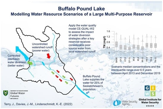
The total spread of predicted concentrations at segment 86 illustrates the overall impact on water quality concentrations per scenario (Figure 8). For DOC, TP, and TN results for all scenarios and the base model appear positively skewed. This data distribution infers that most predicted concentrations were small (the box plus left tail includes 75% of the predicted concentrations). The whiskers in Figure 8 are plotted at interquartile range (IQR) ∗ 1.5, with the remaining data, beyond the whiskers, representing the infrequent high concentration loading events (e.g., freshet). TDS demonstrated increasing skewness with the duration of LDief releases and increased transfer rates.
The constant flow and immediate release scenarios show a decrease in the median value and the IQR range for both TDS, DOC, and TN over the base model. This indicates that predicted concentrations over the model period were lowered by the LDief water transfers. TP displayed opposite behaviour to the other constituents, which may in part be a result of the transformation equation applied to PO43−-P in the LDief constituent file. Overall, CHLA did not change greatly from the base model due to scenario predictions showing both increases and decreases in concentrations over the simulation period, as per the time series plots.
In the timed release scenario, the LDief water was released for only 306 days (12.4% of days) with the rest of the inflows the same as the base model. This shorter duration of water transfers did not alter the overall median and IQR as markedly as the other two scenarios. Segment 86 results from the timed release scenario (Figure 7) suggest that, if the water transfers had been repeated once the 2015 freshet had subsided and continued between the subsequent freshets, then the medians and IQR range may have been much lower. Such a scenario would have been similar to the immediate release scenario but with transfers stopped temporarily each year during flood periods.
Overall, the scenario results implied that adding additional transfers of water from LDief resulted in a greater number of days with lower levels of nutrients. As we anticipated, the influx of better-quality source water from LDief improved the general water quality of BPL. The constant flow scenario appeared to be the most effective at lowering total concentrations in the plotted segments at all three transfer rates.
At the same time, the increased discharge transported constituents more rapidly and further through the lake during peak events. This created shorter, more frequent peaks at the location of the BPWTP intake pipe than occurred with the base model—with the freshet nutrient peaks arriving earlier in the season. These results are consistent with the decrease in residence time and increased flow velocity from adding the additional discharge volume in the scenarios. The timed release scenario results, at segment 86 for the 2015 freshet, suggest that pausing the water transfers during periods of high flow may reduce the intensity of the nutrient peak arriving at the BPWTP intake location. It may be that trying to push as much water as one can at any time is not always effective at attaining water quality goals. In addition, pausing the water transfers during high flow events will need to occur to ensure flows remain within the Upper Qu’Appelle’s channel capacity.
4. Concluding Remarks
Stakeholder engagement at the model design stage helps give confidence in the modelling process and end results. Workshops have shown that end users have a better understanding of what is being modelled, modelling possibilities and limitations, e.g., [54,55]. Stakeholders are more satisfied with output because model scenarios have been tailored to meet their own specific objectives. In this study, the provincial water management agency, the WSA, was provided with the opportunity to refine the scope of the model development and scenarios in order to address pertinent questions about water diversion strategy. For example, the WSA were keen to incorporate the extension to the model bathymetry to remove uncertainties in results brought to light in earlier studies, e.g., [32]. In turn, the enhanced in-lake water quality sampling by the WSA allowed this bathymetry to be implemented and tested in the model. The result was a more robust model that satisfies both stakeholder and scientific objectives. With this study we are bridging the needs of the end user and water quality modelling.
The modelled results show that, dependent on the timing and quantity of water transferred, the increased volume of water is predicted to decrease some water quality parameters in BPL. A flow rate of 12 m3/s was most effective at lowering total concentrations for all scenarios. BPL’s residence time is highly variable and scenario results indicate that the lake will respond rapidly to increased discharge velocity. The expansion of the model grid, and inclusion of the newer profile data, removed the uncertainties existing in the original BPL model with regards to hydrology and transport. There is strong support that the timing of LDief water transfers is important. Results for the timed release scenario suggest the optimum timing would be to wait until overland runoff is at a minimum before commencing water transfers, followed by terminating transfers before runoff resurges. Constituent concentrations near the treatment plant intake are lowest during the 2015 freshet for this scenario (Figure 7). Another benefit to this approach is that the risk of flooding the Upper Qu’Appelle system during natural high runoff events is reduced.
The difference in TP behaviour with and without the transformation equation underscores the need to understand how constituents change along the Upper Qu’Appelle before releasing any transfers. Such a study would require higher-frequency sampling data along the Upper Qu’Appelle than is available at present. Options include extending the W2 model upstream to LDief, or the coupling of two or more water quality models in a river–lake chain. The simulations in this study were based on current environmental conditions and should be treated with caution for long-term planning. Climate is changing in the Prairies and the climate change signal may eventually outweigh the benefits of releasing additional water from LDief. Testing the flow management options under climate change simulations will be the next step for the BPL model.
Author Contributions
Conceptualization, J.T., J.-M.D. and K.-E.L.; Formal analysis, J.T.; Funding acquisition, K.-E.L.; Investigation, J.T. and J.-M.D.; Methodology, J.T. and J.-M.D.; Supervision, K.-E.L.; Visualization, J.T.; Writing—original draft, J.T.; Writing—review & editing, J.-M.D. and K.-E.L. All authors have read and agreed to the published version of the manuscript.
Funding
Funding for this project was provided by the University of Saskatchewan’s Global Water Futures Program.
Acknowledgments
The authors thank the Buffalo Pound Water Treatment Plant and the Saskatchewan Water Security Agency for providing water quality data used to build and verify the model. The University of Saskatchewan’s School of Environment and Sustainability and Global Institute for Water Security also provided data and technical support. Analyses presented in this paper do not necessarily reflect the opinions or official position of the Saskatchewan Water Security Agency or the Government of Saskatchewan.
Conflicts of Interest
The authors declare no conflict of interest. The funders had no role in the design of the study; in the collection, analyses, or interpretation of data; in the writing of the manuscript, or in the decision to publish the results.
References
- Castelletti, A.; Yajima, H.; Giuliani, M.; Soncini-Sessa, R.; Weber, E. Planning the Optimal Operation of a Multioutlet Water Reservoir with Water Quality and Quantity Targets. J. Water Resour. Plan. Manag. 2014, 140, 496–510. [Google Scholar] [CrossRef] [Green Version]
- Zheng, T.; Sun, S.; Liu, H.; Xia, Q.; Zong, Q. Optimal control of reservoir release temperature through selective withdrawal intake at hydropower dam. Water Sci. Technol. Water Supply 2017, 17, 279–299. [Google Scholar] [CrossRef] [Green Version]
- Carr, M.K.; Sadeghian, A.; Lindenschmidt, K.-E.; Rinke, K.; Morales-Marin, L. Impacts of Varying Dam Outflow Elevations on Water Temperature, Dissolved Oxygen, and Nutrient Distributions in a Large Prairie Reservoir. Environ. Eng. Sci. 2019, 37, 78–97. [Google Scholar] [CrossRef] [PubMed] [Green Version]
- Weber, M.; Boehrer, B.; Rinke, K. Minimizing environmental impact whilst securing drinking water quantity and quality demands from a reservoir. River Res. Appl. 2019, 35, 365–374. [Google Scholar] [CrossRef]
- Zhang, C.; Gao, X.; Wang, L.; Chen, Y. Analysis of agricultural pollution by flood flow impact on water quality in a reservoir using a three-dimensional water quality model. J. Hydroinform. 2013, 15, 1061–1072. [Google Scholar] [CrossRef]
- Mamani Larico, A.J.; Zúñiga Medina, S.A. Application of WASP model for assessment of water quality for eutrophication control for a reservoir in the Peruvian Andes. Lakes Reserv. Res. Manag. 2019, 24, 37–47. [Google Scholar] [CrossRef] [Green Version]
- Ziemińska-Stolarska, A.; Kempa, M. Modeling and monitoring of hydrodynamics and surface water quality in the sulejów dam reservoir, poland. Water 2021, 13, 296. [Google Scholar] [CrossRef]
- Jeznach, L.C.; Hagemann, M.; Park, M.-H.; Tobiason, J.E. Proactive modeling of water quality impacts of extreme precipitation events in a drinking water reservoir. J. Environ. Manag. 2017, 201, 241–251. [Google Scholar] [CrossRef]
- Morales-Marín, L.A.; Wheater, H.S.; Lindenschmidt, K.E. Assessment of nutrient loadings of a large multipurpose prairie reservoir. J. Hydrol. 2017, 550, 166–185. [Google Scholar] [CrossRef]
- Deus, R.; Brito, D.; Mateus, M.; Kenov, I.; Fornaro, A.; Neves, R.; Alves, C.N. Impact evaluation of a pisciculture in the Tucuruí reservoir (Pará, Brazil) using a two-dimensional water quality model. J. Hydrol. 2013, 487, 1–12. [Google Scholar] [CrossRef]
- Jeznach, L.C.; Jones, C.; Matthews, T.; Tobiason, J.E.; Ahlfeld, D.P. A framework for modeling contaminant impacts on reservoir water quality. J. Hydrol. 2016, 537, 322–333. [Google Scholar] [CrossRef]
- Akomeah, E.; Morales-Marın, L.A.; Carr, M.; Sadeghian, A.; Lindenschmidt, K.E. The impacts of changing climate and streamflow on nutrient speciation in a large Prairie reservoir. J. Environ. Manag. 2021, 288, 112262. [Google Scholar] [CrossRef] [PubMed]
- Shiklomanov, I.A. Appraisal and assessment of world water resources. Water Int. 2000, 25, 11–32. [Google Scholar] [CrossRef]
- Simonovic, S.P.; Rajasekaram, V. Integrated analyses of Canada’s Water resources: A system dynamics approach. Can. Water Resour. J. 2004, 29, 223–250. [Google Scholar] [CrossRef]
- Wheater, H.; Gober, P. Water security in the Canadian Prairies: Science and management challenges. Philosophical transactions. Ser. A Math. Phys. Eng. Sci. 2013, 371, 20120409. [Google Scholar] [CrossRef]
- Martz, L.; Bruneau, J.; Rolfe, J. Climate Change and Water: SSRB (South Saskatchewan River Basin) Final Technical Report; University of Saskatchewan: Saskatoon, SK, Canada, 2007. [Google Scholar]
- Patrick, R.J. Enhancing water security in Saskatchewan, Canada: An opportunity for a water soft path. Water Int. 2011, 36, 748–763. [Google Scholar] [CrossRef]
- Gober, P.; Wheater, H.S. Socio-hydrology and the science-policy interface: A case study of the Saskatchewan River basin. Hydrol. Earth Syst. Sci. 2014, 18, 1413–1422. [Google Scholar] [CrossRef] [Green Version]
- Diamond, L. Comparative Approaches in Lake Management Planning (Chandos and Buffalo Pound Lake, Canada). Landsc. J. 1984, 3, 61–71. [Google Scholar] [CrossRef]
- Davis, E.; Sauer, E.K. Water Quality Deterioration During Interbasin Transfer in Saskatchewan. Can. Water Resour. J. 1988, 13, 50–59. [Google Scholar] [CrossRef] [Green Version]
- McGowan, S.; Leavitt, P.; Hall, R. A Whole-Lake Experiment to Determine the Effects of Winter Droughts on Shallow Lakes. Ecosystems 2005, 8, 694–708. [Google Scholar] [CrossRef]
- Kehoe, M.; Chun, K.; Baulch, H. Who Smells? Forecasting Taste and Odor in a Drinking Water Reservoir. Environ. Sci. Technol. 2015, 49, 10984. [Google Scholar] [CrossRef] [PubMed]
- Hosseini, N.; Akomeah, E.; Davis, J.-M.; Baulch, H.; Lindenschmidt, K.-E. Water quality modeling of a prairie river-lake system. Environ. Sci. Pollut. Res. Int. 2018, 25, 31190–31204. [Google Scholar] [CrossRef] [PubMed]
- Cavaliere, E.; Baulch, H.M. Winter in two phases: Long-term study of a shallow reservoir in winter. Limnol. Oceanogr. 2021, 66, 1335–1352. [Google Scholar] [CrossRef]
- Barica, J. Water Quality Problems Associated with High Productivity of Prairie Lakes in Canada: A Review. Water Qual. Bull. 1987, 12, 107–115. [Google Scholar]
- Donald, D.B.; Parker, B.R.; Davies, J.-M.; Leavitt, P.R. Nutrient sequestration in the Lake Winnipeg watershed. J. Great Lakes Res. 2015, 41, 630–642. [Google Scholar] [CrossRef]
- North, R.L.; Davies, J.-M.; Doig, L.E.; Lindenschmidt, K.-E.; Hudson, J.J. Lake Diefenbaker: The prairie jewel. J. Great Lakes Res. 2015, 41, 1–7. [Google Scholar] [CrossRef] [Green Version]
- Acharya, M.; Kells, J.A. Conveyance capacity investigations for the Upper Qu’Appelle River Channel. In Proceedings of the 17th Canadian Hydrotechnical Conference, Edmonton, AB, Canada, 17–19 August 2015. [Google Scholar]
- Parsons, G.F.; Thorp, T.; Kulshreshtha, S.; Gates, C. Upper Qu’Appelle Water Supply Project: Economic Impact & Sensitivity Analysis; Clifton Associates Ltd.: Regina, SK, Canda, 2012; p. 101. [Google Scholar]
- Lindenschmidt, K.-E.; Davies, J.-M. Winter flow testing of the Upper Qu’Appelle River. In Proceedings of the 17th CRIPE Workshop on the Hydraulics of Ice Covered Rivers, Edmonton, AB, Canada, 21–24 July 2013; pp. 312–328. [Google Scholar]
- Lindenschmidt, K.-E.; Carstensen, D. The upper Qu’Appelle water supply project in Saskatchewan, Canada: Upland canal ice study. Osterr. Wasser Abfallwirtsch. 2015, 67, 230–239. [Google Scholar] [CrossRef]
- Terry, J.A.; Lindenschmidt, K.-E. Sensitivity of boundary data in a shallow prairie lake model. Can. Water Resour. J. 2020, 45, 204–215. [Google Scholar] [CrossRef]
- Environment and Climate Change Canada. Climate Normals 1981–2010 Station Data for Moose Jaw A Station. Available online: http://climate.weather.gc.ca (accessed on 21 November 2014).
- Water Security Agency. Dams & Reservoirs. Available online: https://www.wsask.ca/lakes-rivers/dams-reservoirs/ (accessed on 3 October 2021).
- Sauchyn, D.J.; Barrow, E.M.; Hopkinson, R.F.; Leavitt, P.R. Aridity on the Canadian Plains. Géographie Phys. Et Quat. 2002, 56, 247–259. [Google Scholar] [CrossRef] [Green Version]
- Chun, K.P.; Wheater, H.S.; Nazemi, A.; Khaliq, M.N. Precipitation downscaling in Canadian Prairie Provinces using the LARS-WG and GLM approaches. Can. Water Resour. J. 2013, 38, 311–332. [Google Scholar] [CrossRef]
- Buffalo Pound Water Administration Board. Annual Report 2015. Available online: https://www.buffalopoundwtp.ca/images/docs/2015_buffalo_pound_annual_report.pdf (accessed on 19 July 2017).
- Wells, S.A. CE-QUAL-W2: A Two-Dimensional, Laterally Averaged, Hydrodynamic and Water Quality Model, Version 4.2, User Manual, Parts 1–5; Department of Civil and Environmental Engineering, Portland State University: Portland, OR, USA, 2020. [Google Scholar]
- Terry, J.A.; Sadeghian, A.; Lindenschmidt, K.-E. Modelling Dissolved Oxygen/Sediment Oxygen Demand under Ice in a Shallow Eutrophic Prairie Reservoir. Water 2017, 9, 131. [Google Scholar] [CrossRef] [Green Version]
- Vandergucht, D.M.; Perez-Valdivia, C.; Davies, J.-M. Qu’Appelle Nutrient Mass Balance Report 2013–2016; Report WQ201812-01; Water Security Agency: Moose Jaw, SK, Canada, 2018.
- Terry, J.A.; Sadeghian, A.; Baulch, H.M.; Chapra, S.C.; Lindenschmidt, K.-E. Challenges of modelling water quality in a shallow prairie lake with seasonal ice cover. Ecol. Model. 2018, 384, 43–52. [Google Scholar] [CrossRef]
- Newbold, J.D.; Elwood, J.W.; O’Neill, R.V.; Winkle, W.V. Measuring Nutrient Spiralling in Streams. Can. J. Fish. Aquat. Sci. 1981, 38, 860–863. [Google Scholar] [CrossRef]
- Ensign, S.H.; Doyle, M.W. Nutrient spiraling in streams and river networks. J. Geophys. Res. Biogeosci. 2006, 111, G04009. [Google Scholar] [CrossRef]
- Lindenschmidt, K.-E. Winter Flow Testing of the Upper Qu’Appelle River; Lambert Academic Publishing: Saarbrucken, Germany, 2014. [Google Scholar]
- House, W.A. Geochemical cycling of phosphorus in rivers. Appl. Geochem. 2003, 18, 739–748. [Google Scholar] [CrossRef]
- Jarvie, H.P.; Jürgens, M.D.; Williams, R.J.; Neal, C.; Davies, J.J.L.; Barrett, C.; White, J. Role of river bed sediments as sources and sinks of phosphorus across two major eutrophic UK river basins: The Hampshire Avon and Herefordshire Wye. J. Hydrol. 2005, 304, 51–74. [Google Scholar] [CrossRef]
- Bowes, M.J.; House, W.A.; Hodgkinson, R.A. Phosphorus dynamics along a river continuum. Sci. Total Environ. 2003, 313, 199–212. [Google Scholar] [CrossRef]
- Butler, B.A.; Ford, R.G. Evaluating Relationships Between Total Dissolved Solids (TDS) and Total Suspended Solids (TSS) in a Mining-Influenced Watershed. Mine Water Environ. 2018, 37, 18–30. [Google Scholar] [CrossRef]
- Rohlfs, A.-M.; Mitrovic, S.M.; Williams, S.; Hitchcock, J.N.; Rees, G.N. Dissolved organic carbon delivery from managed flow releases in a montane snowmelt river. Aquat. Sci. 2016, 78, 793–807. [Google Scholar] [CrossRef]
- Hernes, P.J.; Spencer, R.G.M.; Dyda, R.Y.; Pellerin, B.A.; Bachand, P.A.M.; Bergamaschi, B.A. The role of hydrologic regimes on dissolved organic carbon composition in an agricultural watershed. Geochim. Et Cosmochim. Acta 2008, 72, 5266–5277. [Google Scholar] [CrossRef]
- Fulweiler, R.W.; Nixon, S.W. Export of Nitrogen, Phosphorus, and Suspended Solids from a Southern New England Watershed to Little Narragansett Bay. Biogeochemistry 2005, 76, 567–593. [Google Scholar] [CrossRef]
- Terry, J.A.; Mc Benskin, C.; Eastoe, E.F.; Haygarth, P.M. Temporal dynamics between cattle in-stream presence and suspended solids in a headwater catchment. Environ. Sci. Processes Impacts 2014, 16, 157–1577. [Google Scholar] [CrossRef] [PubMed]
- Perks, M.T.; Owen, G.J.; Benskin, C.M.H.; Jonczyk, J.; Deasy, C.; Burke, S.; Reaney, S.M.; Haygarth, P.M. Dominant mechanisms for the delivery of fine sediment and phosphorus to fluvial networks draining grassland dominated headwater catchments. Sci. Total Environ. 2015, 523, 178–190. [Google Scholar] [CrossRef] [PubMed] [Green Version]
- Hassanzadeh, E.; Strickert, G.; Morales-Marin, L.; Noble, B.; Baulch, H.; Shupena-Soulodre, E.; Lindenschmidt, K.-E. A framework for engaging stakeholders in water quality modeling and management: Application to the Qu’Appelle River Basin, Canada. J. Environ. Manag. 2019, 231, 1117–1126. [Google Scholar] [CrossRef]
- Lindenschmidt, K.-E.; Akomeah, E.; Baulch, H.; Boyer, L.; Davies, J.-M.; Hassanzadeh, E.; Marin, L.M.; Strickert, G.; Wauchope, M. Interfacing Stakeholder Involvement into a Surface Water-Quality Modelling System for Water Management and Policy Development. In New Trends in Urban Drainage Modelling; Springer: Berlin/Heidelberg, Germany, 2019; pp. 312–316. [Google Scholar]
Figure 1.
Left: The Upper Qu’Appelle watershed. Right: Buffalo Pound Lake (BPL), Saskatchewan, Canada. The lake has a mean depth of 3.8 m, maximum depth of 6.0 m, average width of 890 m, and total length of 30 kms. Red circles are the water quality sampling stations and green circles are the flow gauges used in this study. Hwy #2 and #19 are official highway numbers.

Figure 2.
Left: Model grid with longitudinal segmentation. The upstream area in the red circle is the newly extended section of the model. Right: New digital elevation model of BPL including the upper shallow section of lake. Depths are shown relative to operating full supply level.
Figure 2.
Left: Model grid with longitudinal segmentation. The upstream area in the red circle is the newly extended section of the model. Right: New digital elevation model of BPL including the upper shallow section of lake. Depths are shown relative to operating full supply level.

Figure 3.
Regression plots for the three constituents that displayed a stronger relationship (adjusted R square > 0.5) between change in concentrations during transport along the Upper Qu’Appelle River with flow rate. Flow is average daily flow in m3/s at the WSA gauging station Elbow Diversion.
Figure 3.
Regression plots for the three constituents that displayed a stronger relationship (adjusted R square > 0.5) between change in concentrations during transport along the Upper Qu’Appelle River with flow rate. Flow is average daily flow in m3/s at the WSA gauging station Elbow Diversion.

Figure 4.
Model results for BPL for the calibration period April 2013–December 2019. Segment 5 is located upstream in the top section of lake. Segments 32 and 86 are both located in the main body of the lake. Water Security Agency observed in-lake sample data (red *) are included from June 2015. Observed weekly data provided by the Buffalo Pound Water Treatment Plant (green +) are shown in segment 86. Inflow constituents DO = dissolved oxygen, and CHLA = Chlorophyll-a.

Figure 5.
Output for five model-derived water quality constituents of interest at segments 5, 32 and 86 for the constant flow scenario. Scenario flow rates for the water transfers are 4, 8 and 12 m3/s.
Figure 5.
Output for five model-derived water quality constituents of interest at segments 5, 32 and 86 for the constant flow scenario. Scenario flow rates for the water transfers are 4, 8 and 12 m3/s.

Figure 6.
Output for five model-derived water quality constituents of interest at segments 5, 32 and 86 for the immediate release scenario.
Figure 6.
Output for five model-derived water quality constituents of interest at segments 5, 32 and 86 for the immediate release scenario.

Figure 7.
Output for five model-derived water quality constituents of interest at segments 5, 32 and 86 for the timed release scenario.
Figure 7.
Output for five model-derived water quality constituents of interest at segments 5, 32 and 86 for the timed release scenario.

Figure 8.
Boxplots comparing model output at segment 86 for the base model and the nine simulation runs for April 2013–December 2019. The box represents 50% of the ranked data (interquartile range, or IQR) with the median marked as a horizontal line within the box. Whiskers represent upper and lower bounds at (IQR ∗ factor of ±1.5).


Table 1.
Main coefficients used in the water quality model (previous model rates in parentheses if changed) from Terry and Lindenschmidt [32]).
Table 1.
Main coefficients used in the water quality model (previous model rates in parentheses if changed) from Terry and Lindenschmidt [32]).
| Coefficient | Description | Value | Units | |
| TSED | Sediment temperature | 10.3 | °C | |
| CBHE | Coefficient of bottom heat exchange | 0.3 | W m−2 | |
| SOD | Zero-order sediment oxygen demand | 0.1–1.2 (1.2) | g O2 m−2 day−1 | |
| PO4R | Sediment release rate of phosphorus (fraction of SOD) | 0.001 | ||
| NH4R | Sediment release rate of ammonium (fraction of SOD) | 0.001 | - | |
| NH4DK | Ammonium decay rate | 0.12 | day−1 | |
| NO3DK | Nitrate decay rate | 0.1 | day−1 | |
| LDOMDK | Labile DOM decay rate | 0.1 (0.25) | day−1 | |
| RDOMDK | Refractory DOM decay rate | 0.001 (0.012) | day−1 | |
| LRDDK | Labile to refractory DOM decay rate | 0.01 (0.001) | day−1 | |
| LPOMDK | Labile POM decay rate | 0.08 (0.32) | day−1 | |
| RPOMDK | Refractory POM decay rate | 0.001 (0.012) | day−1 | |
| LRPDK | Labile to refractory POM decay rate | 0.01 | day−1 | |
| SSS | Suspended solids settling rate | 1.0 | m day−1 | |
| EXSS | Extinction due to inorganic suspended solids | 0.01 | m−1/(g m−3) | |
| EXOM | Extinction due to organic suspended solids | 0.01 | m−1/(g m−3) | |
| EXH20 | Light extinction coefficient for pure water | 0.25 | m−1 | |
| BETA | Fraction of incident solar radiation absorbed at the water surface | 0.55 | - | |
| WSC | Wind shelter coefficient | 0.9 | °C | |
| Algal Coefficients | Diatoms | Greens | Cyanobacteria | |
| AG | Maximum algal growth rate, day−1 | 1.5 (2.5) | 2.0 (1.0) | 0.5 (0.9) |
| AM | Maximum algal mortality rate, day−1 | 0.1 | 0.1 (0.15) | 0.1 |
| AS | Algal settling rate, m day−1 | 0.2 (0.02) | 0.1 (0.15) | 0.02 (0.1) |
| AHSP | Algal half-saturation for phosphorus limited growth, g m−3 | 0.003 | 0.003 | 0.003 |
| AHSN | Algal half-saturation for nitrogen limited growth, g m−3 | 0.014 | 0.014 | 0 * (0.01) |
| AT1 | Lower temperature for algal growth, °C | 2.0 | 10.0 | 10.0 |
| AT2 | Lower temperature for maximum algal growth, °C | 8.0 | 30.0 | 35.0 |
| AT3 | Upper temperature for maximum algal growth, °C | 15.0 | 35.0 | 40.0 |
| AT4 | Upper temperature for algal growth, °C | 24.0 | 40.0 | 50.0 |
| ACHLA | Ratio between algal biomass and chlorophyll a in terms of mg algae/µg chl a | 0.05 | 0.04 | 0.1 |
* Denotes nitrogen fixation–Dolichospermum spp. (formerly Anabaena) are one of the dominant cyanobacteria taxa in BPL.
Table 2.
Regression models of the net change in concentration values for constituents travelling along the Upper Qu’Appelle River, as a function of flow at the upstream Elbow Diversion gauging station. Constituents are total suspended solids (TSS), total phosphorus (TP), orthophosphate (PO43−-P), dissolved organic carbon (DOC), total dissolved solids (TDS), ammonium (NH4-N), total nitrogen (TN) and nitrate-nitrite (NOx). Flow is average daily flow in m3/s and constituents are in mg/L.
| Observations | Adjusted R Square | Standard Error | p-Value (Flow) | p-Value (Intercept) | |
|---|---|---|---|---|---|
| TSS (TSS = 24.600 ∗ Flow − 3.880) | 40 | 0.567 | 61.756 | <0.001 | 0.808 |
| TP (ΔTP = 0.025 ∗ Flow − 0.008) | 40 | 0.540 | 0.067 | <0.001 | 0.655 |
| PO43−-P (ΔPO43−-P= 0.007 ∗ Flow − 0.002) | 8 | 0.511 | 0.019 | <0.05 | 0.828 |
| DOC (ΔDOC = −0.262 ∗ Flow + 2.064) | 40 | 0.133 | 1.798 | <0.05 | <0.001 |
| TDS (ΔTDS = −42.700 ∗ Flow + 331.88) | 40 | 0.123 | 303.886 | <0.05 | <0.001 |
| NH4-N (ΔNH4-N = −0.389 ∗ Flow + 3.256) | 8 | 0.051 | 2.722 | 0.286 | 0.080 |
| TN (ΔTN = 0.023 ∗ Flow + 0.003) | 40 | 0.032 | 0.278 | 0.138 | 0.969 |
| NOx (ΔNOx = −0.002 ∗ Flow − 0.01) | 23 | −0.030 | 0.046 | 0.551 | 0.610 |
Publisher’s Note: MDPI stays neutral with regard to jurisdictional claims in published maps and institutional affiliations. |
© 2022 by the authors. Licensee MDPI, Basel, Switzerland. This article is an open access article distributed under the terms and conditions of the Creative Commons Attribution (CC BY) license (https://creativecommons.org/licenses/by/4.0/).
Share and Cite
MDPI and ACS Style
Terry, J.; Davies, J.-M.; Lindenschmidt, K.-E. Buffalo Pound Lake—Modelling Water Resource Management Scenarios of a Large Multi-Purpose Prairie Reservoir. Water 2022, 14, 584. https://doi.org/10.3390/w14040584
AMA Style
Terry J, Davies J-M, Lindenschmidt K-E. Buffalo Pound Lake—Modelling Water Resource Management Scenarios of a Large Multi-Purpose Prairie Reservoir. Water. 2022; 14(4):584. https://doi.org/10.3390/w14040584
Chicago/Turabian StyleTerry, Julie, John-Mark Davies, and Karl-Erich Lindenschmidt. 2022. "Buffalo Pound Lake—Modelling Water Resource Management Scenarios of a Large Multi-Purpose Prairie Reservoir" Water 14, no. 4: 584. https://doi.org/10.3390/w14040584
Note that from the first issue of 2016, this journal uses article numbers instead of page numbers. See further details here.