Article

Water Use and Soil Water Balance of Mediterranean Vineyards under Rainfed and Drip Irrigation Management: Evapotranspiration Partition and Soil Management Modelling for Resource Conservation

1
Landscape Environment Agricultural and Food (LEAF), Institute of Agronomy, University of Lisbon, Tapada da Ajuda, 1349-017 Lisbon, Portugal
2
Centro de Ciência e Tecnologia do Ambiente e do Mar (MARETEC), LARSyS, Instituto Superior Técnico, University of Lisbon, Av. Rovisco Pais, 1, 1049-001 Lisbon, Portugal
3
Istituto di Scienze e Tecnologie per l’Energia e la Mobilità Sostenibili (STEMS), Consiglio Nazionale delle Ricerche (CNR), 10135 Torino, Italy
*
Author to whom correspondence should be addressed.
Water 2022, 14(4), 554; https://doi.org/10.3390/w14040554
Submission received: 17 December 2021 / Revised: 28 January 2022 / Accepted: 10 February 2022 / Published: 12 February 2022

Abstract

:
Vineyards represent complex Mediterranean agrosystems that deliver significant ecosystem services to society. Yet, many vine-growers still need to assimilate the importance of crop and soil management to the conservation of soil and water resources. The main objective of this study was to evaluate water use and the water balance terms in rainfed and irrigated vineyards in Italy and Portugal, respectively, in both cases aiming at the sustainability of natural resources use. The SIMDualKc model is used for both sites after calibration and validation by fitting soil water content measurements. The Italian case study focused on the impacts of inter-row conservation management in hillslope vineyards while the Portuguese case study analyzed irrigation water management under scarcity in flat vineyards. For the Italian vineyards, the model results focused on the evapotranspiration fluxes and their partition, control of surface runoff, and soil water recharge provided by the inter-row soil management using cover crops. Model results of the Portuguese case study showed the need for improving irrigation water use and the terms of water balance, namely referring to percolation and soil water evaporation. Both case studies further demonstrated the advantages of using computational tools to better cope with climate variability in the Mediterranean region and made evident the benefits of improved crop and soil management practices in counteracting land degradation and valuing the use and conservation of natural resources.

1. Introduction

Viticulture is one of the most diffused cultivations in the world and has been practiced in the Mediterranean area for millennia [1]. In this region, the vineyard agricultural system is potentially well suited for delivering provisioning services such as grapes for table or wine production, the regulation of climate and the hydrologic cycle [2], and the preservation and enhancement of cultural heritage including landscape and aesthetic values [3,4]. Contrasting, vineyards are often associated with several environmental problems resulting from the intensification of production systems, which evidence the need for better management of soil and water resources.
There is abundant bibliography relative to soil management, namely in sloping fields in sub-humid to humid climates. Salomé et al. [5] provided a review based on 146 commercial plots and focused on three soil management practices: inter-row plant cover, weeding, and fertilization strategies. Fertilization contributes to improve yields and, therefore, to a higher water productivity while weeding has different impacts depending on whether it is performed mechanically or chemically. Both practices are influenced by the soil type. Mechanical weeding often contributes to runoff and erosion, mainly when intense rainfall occurs and when the soil structure is poor with unstable aggregates. Differently, a cover crop in the inter row, even temporary, benefits soil functioning whatever the soil type. The superiority of adopting a cover crop in the inter-row is reported by many authors, e.g., Biddoccu et al. [6,7] relative to control both soil erosion and runoff in sloping fields. Research results reported by Gómez et al. [8], Prosdocimi et al. [9], and Capello et al. [10] confirm those results. Plant cover contributes to retardation and control of runoff, water infiltration, reduction of soil erosion, increase in organic matter (OM), carbon sequestration, and nutrient supply and retention [5,11,12]. However, the ground cover plants generally compete for water with the vine plants and require special care in water scarce areas.
Inter-row management influences the response of the vineyard to different types of rainfall events, namely in terms of rainwater partition between infiltration and runoff, thus influencing the amount of soil erosion. It further impacts the whole field water balance as well as vines nutrition, growth, and productivity [13,14]. The importance of cover crops to control soil erosion is great, with decreasing soil losses up to 75%, but competition for water and nutrients by the cover crop may reduce yields by up to 54% [11]. Napoli et al. [12] reported for cover crops 68.5% less soil losses than in inter-rows with harrowed soil. Capello et al. [10] reported that grass cover reduced runoff by 65%, and soil erosion losses by 72%. In addition, the response of grass cover plot was less influenced by traffic conditions. In fact, the increased mechanization in vineyards is frequently associated with increased soil compaction due to repeated tractor passes on fixed paths [10,15], which increases runoff and soil erosion, mainly in sloping vineyards. This soil loss is particularly important when the soil is left bare in the inter-row and exposed to intense rainfall events [16,17]. Such question highlights the importance of inter-row management for the sustainability of the use of natural resources by the vineyard system. Biddoccu et al. [6] also reported on a 10-year field research in 15% sloping fields finding that the highest soil losses were observed for conventional and reduced tillage, respectively, 111.5 and 207.7 Mg ha−1 while losses were only 25.6 Mg ha−1 for the grass covered (GC) treatment. The worst soil management practice was reduced tillage. Keesstra et al. [18] reported that vegetation cover, soil moisture, and organic matter were significantly higher in covered plots than in tilled and herbicide treated plots, while sediment yield and soil erosion were significantly higher in herbicide treated plots. Nevertheless, as reported by Biddoccu et al. [7], adopting temporary cover crops may not produce the target effects on soil protection. In addition, the protection role of the cover crop depends on the grass type, e.g., with temporary natural vegetation being less efficient than saifoin [19].
Novara et al. [14] reported that the use of cover crops is a strategy that may positively influence water productivity by reducing excessive vines vigor in fertile soils and/or favoring deeper roots in layers. However, in low vigor vineyards, low fertile soils, and in dry environments, the competition for water needs to be considered to avoid negative impacts on yields. Moreover, for Mediterranean ecosystems, attention should be paid to their impact on water availability [14]. The use of cover crops in the inter-row provides various ecosystem services including reduction of runoff and erosion and improvement of water supply. Thus, permanent cover crops are commonly implemented in Europe where climate is not excessively dry [7,20,21,22]. Differently, in semi-arid Mediterranean regions, winegrowers are reluctant to use cover crops due to concerns over soil water competition [23,24]. The competition for soil water at critical crop stages can lead to excessive grapevine water stress, reducing the fruit set, causing premature defoliation, and negatively impacting growth, yields, and the quality of berries [25,26]. In this perspective, it is crucial to know the response of vineyards to rainfall distribution in terms of water availability to plants when considering the presence of cover crops in the inter-row, both in rainfed and irrigated vineyards, since the dynamics of evapotranspiration and water use is insufficiently known in both cases. Moreover, related measures and practices are among those required for adaptation and resilience to climate change impacts.
Costa et al. [27] assumed a long-term perspective when focusing on genetics, selection of varieties and plant amelioration of both the grapevines and the rootstocks, aimed at improving grapevine responses to heat stress and drought, thus in addition to the measures and practices reported. These authors largely referred to policies required to make effective the development of farm responses of vines to heat and drought and focused on water issues. Moreover, they assumed that future strategies to optimize the environmental performance of the wine sector in the Mediterranean must be focused on water and irrigation. Hannah et al. [28] also assumed that attempting to maintain wine grape productivity and quality under climate change implies increased water use for irrigation and to cool grapes through misting or sprinkling, which creates potential impacts on freshwater conservation. Thus, freshwater habitats may be affected where climate change undermines growing conditions for already established vineyards. Hannah et al. [28] concluded that climate change adaptation strategies are required for creating a positive future for producers, wine makers, and vine ecosystems.
In Italy and Portugal, which represent the 1st and 5th largest wine producers in Europe [29], vineyards were traditionally rainfed since, as in many European countries, irrigation was historically not used, forbidden by regulations for many quality wines. Nowadays, in Italy, many IGT, DOC and DOCG regulations admit only emergency irrigation. However, since the soil water stress strongly affects the growth and production of vines and the quality of berries [30], irrigation has become an increasingly frequent practice especially in dry areas of Southern Europe [31,32]. Yet, poor irrigation practices, namely the inadequacy of irrigation depths to crop water needs, climate, and soil and irrigation system characteristics may cause water percolation and leaching of fertilizers and pesticides, thus not promoting environmental friendliness [33,34,35], nor greater and more stable yields and quality of wine [16]. Better knowledge of the crop water requirements relative to the various crop growth stages are critical to better preserve the vineyards natural resources, namely soil and water.
Accurate knowledge of the soil water balance is fundamental for improving the soil and water management of the vineyard system and to further cope with the challenges resulting from climate change. In Piedmont, Italy, long-term simulations performed over 60 years (1950–2009) confirmed that the climate change is already influencing local vineyards since 1980 [36,37]. Furthermore, Fraga et al. [38] observed that mean phenological timings were projected to undergo significant advancements in Portugal (e.g., budburst and harvest may be anticipated by 1 month or more), with implications also in the corresponding pheno-phase intervals. Impacts of climate change on viticulture likely will be significant [39] in terms of increasing temperature combined with extreme events such as droughts and/or short-term storms [40]. Hence, there is the need for accurate tools for estimating crop water and irrigation requirements, namely soil water balance (SWB) models using weather data and soil water observations and/or other data such as eddy covariance and sap flow data [41,42]. In addition to local ground observations, also remote sensing data may be used in models. Pôças et al. [43] used hyperspectral reflectance data derived from a handheld spectroradiometer to estimate the predawn leaf water potential to assess the water status of grapevine cultivars in the Port wine region to be used in irrigation scheduling. A two-source model was used by Ortega-Farias et al. [44] to estimate vineyard energy balance using thermal images acquired by an unmanned aerial vehicle (UAV). Romero et al. [45] also reported on using multispectral imagery from an UAV platform for water status estimation.
Through modelling, farmers and/or farm advisers use models to support irrigation scheduling under diverse climates and management scenarios. Models may also be used to assess the impact of management decisions on soil and water resources, e.g., SIMDualKc model, which is able to both the partition of crop evapotranspiration (ET) into transpiration and soil evaporation, and the partition of transpiration into the fractions relative to the crop and the understory vegetation [46,47]. Another example is given by Cellete et al. [48] that developed the WaLIS model to simulate water resources partitioning and to estimate ET and the water use for both grapevine and the inter-row cover crop. Phogat et al. [49] applied a Richards-based mechanistic model for computing soil water fluxes and improving agricultural practices in irrigated vineyards, and Kustas et al. [50] and Kool et al. [51] applied the thermal-based two-source energy balance model for monitoring daily ET in vines and the inter-rows. A biosensing IoT platform for water management in vineyards is referred by Loddo et al. [52]. Moreover, there is abundant bibliography for ET studies with grapevines as reviewed by Rallo et al. [53], but not with a cover crop in the inter-row irrigated or rainfed.
The FAO 56 dual-Kc approach is a widely used method that refers to the determination of crop evapotranspiration (ETc) as the product of a Kc value for a specific crop stage and the grass reference evapotranspiration (ETo) computed with the FAO Penman-Monteith equation [54,55]. The Kc value is partitioned into the basal crop coefficient (Kcb) referring to transpiration and the soil evaporation coefficient (Ke), providing thus separate estimates of the ETc components: crop transpiration (Tc) and soil evaporation (Es). Examples of applications to vine and fruit crop systems can be found in the recent literature review provided by Rallo et al. [53] and Pereira et al. [56]. The SIMDualKc model [57] has adopted the dual-Kc approach for estimating daily ET fluxes of crops grown under different climatic regions and management practices, including grapevine [46,47,58], peach [59], and olive [60,61]. Yet, despite the growing use of the FAO56 dual-Kc approach for computing crop evapotranspiration fluxes and improving soil water management in complex agricultural systems, there is still the need for extending research focusing on the search for standard Kc and Kcb values as well the impact of active ground cover, cover crops, and mulches on crop evapotranspiration of vine systems [53].
Considering the insufficient knowledge on vineyards evapotranspiration as related to cover crops, the current study aims to estimate evapotranspiration fluxes and water use in two Mediterranean vineyards, a northern Italy sloping rainfed crop planted in a soil with large soil water holding capacity, and an irrigated one in southern Portugal cropped in a flat area with a sandy soil. Differences between vineyards allow perceiving differences in management and in water responses to both the rainfall regime and the ET. Objectives consist of (i) calibration and validation of the water balance model SIMDualKc [57], already proved for vine and tree crops; (ii) evaluation of the influence of the inter-row cover crop on the evapotranspiration dynamics and the soil water balance of the rainfed vineyard (2016–2019); (iii) evaluation of the evapotranspiration dynamics, the soil water balance, and the irrigation management applied to the drip irrigated vineyard (2018–2020); (iv) with support of the referred model, demonstrating the importance of improved soil and water conservation measures and practices for both Italian and Portuguese cases. The goal of the study focusses on the sustainable use of soil and water resources, thus on the sustainability and resilience of the vineyards production systems taking in account the challenges of climate change.

2. Materials and Methods

2.1. Description of the Study Areas

The Italian case study was located at the “Tenuta Cannona” Experimental Vine and Wine Center of Agrion Foundation (44°40′ N, 8°37′ E, 296 m a.s.l.), in the municipality of Carpeneto (AL), in the southern part of the Monferrato hilly area, known as “Alto Monferrato”, North-West Italy. Data was collected from January 2016 to December 2019. The climate is alpine sublitoranean. According to records from the nearest weather station over the period 1951–1990 (Ovada, 187 m a.s.l.), the average annual precipitation is 965 mm, mainly concentrated in Autumn (October and November) and Spring (March), while the driest month is July [62]. At the experimental site, over the period 2000–2019, the average annual precipitation was slightly lower (881 mm), ranging from a maximum of 1455 mm (2019) to a minimum of 493 mm (2017). The mean annual air temperature was 13 °C (Figure 1). The Cannona vineyards lie on Pleistocenic fluvial terraces in the Tertiary Piedmont Basin, including highly altered gravel, sand, and silty clay deposits, with red alteration products [63]. The main physical characteristics of the studied soils are presented in Table 1. The soils had clay to clay-loam texture and were classified as Dystric Cambisols [64]. Particle size distribution, soil bulk density (ρb), and soil water contents at saturation (θs) and at field capacity (θFC) were obtained from undisturbed soil samples taken at different depths according to Blake and Hartge [65] and Cavazza [66], whereas soil water contents at the wilting point (θWP) were obtained using the Rosetta pedotransfer functions [67] and the particle size distribution and ρb as input (Table 1).
The Portuguese case study was located at Companhia das Lezírias, Samora Correia, southern Portugal (38.808° N, 8.900° W, 45 m a.s.l.). Data were collected from January 2018 to October 2020. The climate in the region is dry sub-humid, with mild winters and hot, dry summers. The mean annual precipitation is 669 mm, mainly concentrated between October and May, while the mean annual temperature is 16.8 °C. The weather data for the study area was obtained from the local weather station and is reported in Figure 2.
The soil was classified as a Haplic Fluvisol [64], with main physical characteristics presented in Table 1. The particle size distribution was obtained using the pipette method for particles having diameters <2 μm (clay fraction) and between 2–20 μm (silt), and by sieving for particles between 20–200 μm (fine sand) and between 200–2000 μm (coarse sand). These textural classes follow the Portuguese classification system [68] and are based on international soil particle limits (Atterberg scale). The dry bulk density (ρb) was obtained by drying volumetric soil samples (100 cm3) at 105 °C for 48 h. The soil water contents at saturation (θs), field capacity (θFC), and the wilting point (θWP) were obtained from pedotransfer functions using the particle size distribution as input [69,70].

2.2. Vineyards Management

As typical in the Monferrato area (Italy), vineyards were rainfed. The experiment was carried out in a vineyard planted in 1988 with Barbera vines, managed according to conventional farming for wine production. Two vineyard plots of 1221 m2 (16.5 m wide and 74 m long) each were considered. Each plot was composed of 6 rows aligned along the slope (SE aspect, average slope 15%), spaced 2.75 m, where the vines were spaced 1.0 m along the row and grown on vertical shoot positioned trellis (VSP). Since 2000, the soil in the two plots has been managed with different techniques: (i) conventional tillage (CT, hereafter) cultivation with chisel (at a depth of about 0.25 m); and (ii) controlled grass cover (GC), i.e., mulching of the spontaneous grass cover. Both practices were usually carried out twice a year, in spring and autumn. Then, the grass cover in the inter-row was mowed additional times during the season, if necessary. Weeds under the rows were controlled with Glyphosate application in spring, on the surface, 0.6 m across the vine row. Wood pruning was carried out in winter, and residues were chipped in one inter-row out of two. Most of the farming operations in the vineyard were carried out using tracked or tyre tractors carrying or towing implements, with intensification of passages from spring to grape harvest time (from 14 to 27 passages per year). The dates of the main crop stages during the four growing seasons are reported in Table 2.
In the 4-years study period, i.e., from January 2016 to December 2019, weather variables, runoff amounts, soil losses, and hourly soil water content related to 89 runoff events were recorded for the two plots. Rainfall, air temperature, and humidity were recorded at 10-min intervals by a weather station placed near the plots. Daily values of solar radiation and wind speed and direction were obtained from stations located 10 km from the vineyard (Acqui Terme, Basaluzzo), belonging to the Regional Environmental Agency [71]. Each vineyard plot was hydraulically “isolated”. The runoff generated by rainfall was collected separately for each plot by a channel connected with a sedimentation trap. A tipping bucket device measured the hourly volumes of runoff (RO, mm) in both CT e GC. Runoff samples were collected to obtain sediment concentration for erosive events, and, if sedimentation occurred in the channels and sediment trap, then the sediment yield was collected and weighted (see Biddoccu et al. [72] for details). Soil water contents were recorded every hour from an average of 1-min by indirect method [73] measurements of capacitance/frequency domain sensors (ECH2O-5TM sensors, Decagon Devices Inc., Pullman, WA, USA), gravimetrically calibrated, placed at 0.1, 0.2, and 0.3 m depth, and stored by a Decagon EM50 datalogger. Soil water content measurements were carried out in the two plots, both in the track position (T), which is the portion of inter-row affected by the passage of tractor wheels or tracks, where the compressive effects tend to concentrate [74], and in the middle of the inter-row, identified as the no-track position (NT), which is not affected by direct contact with tractor wheels or tracks, and then averaged for comparison with model output.
The selected field in Samora Correia (Portugal), planted in 2008, was relatively flat, and part of a larger vineyard (130 ha). The field was a drip-irrigated plot, 5 ha in size, planted with different varieties of wine grapes but where Touriga Nacional was dominant. The plants were grown on VSP trellis, with wood pruning during the dormant period in winter. Plants were at a row distance of 1.0 m and a row spacing of 2.8 m, thus a plant density of approximately 3571 plants ha−1, with an orientation in the east-west direction. The dates of the main crop stages during the three growing seasons can also be found in Table 2. Harvest of grapes in Samora Correia vineyards was performed during September. The inter-row was covered with spontaneous grass from autumn to spring. When necessary, weeds under the rows were controlled with Glyphosate application in spring. Irrigation was delivered through a drip system, with management practices performed according to the standard practices in the region and decided by the farmer. Drippers were spaced 1 m apart, and the drip line was placed on the trellis 0.5 m above the soil surface. The total water applied through irrigation summed 470, 625, and 465 mm in 2018, 2019, and 2020, respectively. The application depth during irrigation events varied from 1 to 12 mm. Soil water contents were continuously monitored in two locations at depths of 10, 20, 30, 40, 50, 60, 70, and 80 cm using EnviroPro MT (MAIT Industries, Australia) capacitance probes. Probes were installed in the crop row, distanced approximately 30 cm from emitters, and measurements were averaged for comparison with model output.

2.3. The SIMDualKc Model

2.3.1. The Soil Water Balance

The SIMDualKc model [57] computes the daily soil water balance at the field scale as follows:
D r , i = D r , i 1 ( P RO ) i I i CR i + DP i + ET c   act , i
where Dr is the root zone depletion (mm), P is the rainfall (mm), RO is the runoff (mm), I is the net irrigation depth (mm), CR is the capillary rise from the groundwater table (mm), DP is the deep percolation (mm), and ETc act is the actual crop evapotranspiration (mm), all referring to day i or i−1. In this study, CR was not considered as the groundwater table was too deep (>5 m) in both case studies and could not contribute to crop evapotranspiration.
The SIMDualKc model adopts the FAO56 dual Kc approach for computing crop evapotranspiration [42,54,55]. In this approach, the components relative to crop transpiration (Tc, mm) and soil evaporation (Es, mm) are computed separately as follows:
T c = K cb   ET o
E s = K e   ET o
where Kcb (-) is the standard basal crop coefficient that refers primarily to crop transpiration although some diffusive soil evaporation may also be included, particularly during the initial crop stage, Ke is the evaporation coefficient (-) that describes direct evaporation from the surface soil layer of depth Ze (cm), and ETo is the reference evapotranspiration (mm) computed with the FAO Penman-Monteith equation [54]. Tc values are reduced when water stress occurs through a multiplier stress coefficient (Ks) to Kcb:
T c   act = K s   K cb   ET o = K cb   act   ET o
where Tc act is the actual crop transpiration (mm) and Kcb act is the actual basal crop coefficient (-). When only the matric potential is constraining Tc values, Ks is computed as follows [42,54]:
K s = TAW     D r , i TAW     RAW
where TAW and RAW are, respectively, the total and readily available soil water relative to the rooting depth (mm). These are computed as:
TAW = 1000   Z r   ( θ FC θ WP )
RAW = p   TAW
where θFC and θWP are the soil water contents at field capacity and the wilting point (m3 m−3), respectively, Zr is the root depth (m), and p (-) is the soil water depletion fraction for no stress. When the depletion exceeds p, i.e., the soil water content drops below RAW, Tc values are reduced due to water stress (Ks < 1.0), otherwise Ks = 1.0.
Soil evaporation is limited by the amount of energy available at the soil surface in conjunction with the energy consumed by transpiration, and by water availability in the surface soil evaporation layer [54,55]. The evaporation coefficient (Ke) is then computed as:
K e = K r ( K c   max K cb   min ) f ew   K c   max
where Kr is the evaporation reduction coefficient (0–1), Kc max is the maximum value of Kc (-) (i.e., Kcb + Ke) following a rain or an irrigation event (−), and few is the fraction of the soil that is both exposed to radiation and wetted by rain or irrigation. few depends upon the effective fraction of ground covered or shaded by vegetation near solar noon (fc eff). Kr is calculated using the two-stage drying cycle approach where the first stage is the energy limited stage, and the second is the water limited stage [42,54,55,75]:
K r = 1   for   D e ,   i 1     REW
K r = TEW     D e , i 1 TEW     REW   for   D e ,   i 1   >   REW
where TEW is the maximum depth of water that can be evaporated from the evaporation soil layer when it has been completely wetted (mm), REW is the depth of water that can be easily evaporated without water availability restrictions (mm), and De is the evaporation layer depletion at the end of day i−1 (mm). De is computed through a daily water balance of the evaporation soil layer, with the evaporation decreasing as the evaporable soil water decreases in the evaporation soil layer beyond REW.
DP is calculated using a time decay function relating the soil water storage near saturation with the time after the occurrence of heavy rain or irrigation [76]:
W a = a D   t b D
where Wa is the actual soil water storage in the root zone (mm), aD is the soil water storage comprised between saturation (θS) and θFC (mm), bD is an empirical dimensionless parameter (-), and t is the time after irrigation or rain that produces storage above field capacity (days). Further information on the estimation of aD and bD is provided by Liu et al. [76].
RO is estimated using the curve number (CN) approach [77], with the CN value depending on the soil type, vegetation type, and antecedent soil moisture. In SIMDualKc, CN is adjusted each day to reflect the impact of increasing or decreasing of the soil water content on soil infiltration properties by relating the CN value to the soil water depletion in the surface layer (De). A different CN value is thus computed according to the correspondence between De and the antecedent soil water conditions AWC I, AWC II, and AWC III (respectively, representing dry, average, and wet soil conditions) [77,78]:
CN = CN I for   D e     D e - AWC   I
CN = CN III for   D e     D e - AWC   III
CN = ( D e 0.5   REW )   CN I + ( 0.7   REW + 0.3   TEW   D e )   CN III 0.2   REW + 0.3   TEW for   D e - AWC   III   <   D e   <   D e - AWC   I
with:
CN I = CN II 2.281 0.01281 CN II
CN III = CN II 0.427 0.00573 CN II
and:
D e AWC   III = 0.5   REW
D e AWC   I = 0.7   REW + 0.3   TEW
where CNI, CNII, and CNIII are, respectively, the curve numbers associated with the antecedent soil water conditions AWC I (dry), AWC II (average), and AWC III (wet) (0–100), and De-AWC I, De-AWC II, and De-AWC III are, respectively, the depletion of the evaporative layer at AWC I, AWC II, and AWC III conditions (mm). CNII corresponds to tabulated values available in USDA-SCS [77] and Allen et al. [78].
The Kcb values are described for four growth stages: the initial stage or start of the crop season, the rapid growth or development stage, the mid-season stage, and the late-season stage. Yet, the Kcb curve is defined by three Kcb values corresponding to the initial (Kcb ini), mid-(Kcb mid), and end-season (Kcb end). For tree crops and vineyards, these are computed based on crop characteristics [42,53,79,80]. When the inter-row has an active ground cover, the Kcb relative to the crop and the understory vegetation may be estimated with the following Equation [57,79]:
K cb = K cb   gcover + K d ( max ( K cb   full K cb   gcover ,   K cb   full   K cb   gcover   2 ) )
where Kcb gcover is the Kcb of the ground cover vegetation in the absence of tree foliage, Kcb full is the estimated basal Kc during peak plant growth for conditions having nearly full ground cover, and Kd is the crop density coefficient. The second term of the max function reduces the estimate for Kcb during the mid-season stage by half the difference between Kcb full and Kcb cover when this difference is negative. This accounts for impacts of the shading of the surface cover by overstory vegetation having a Kcb that is lower than that of the ground cover due to differences in stomatal conductance. When no ground cover exists or when the cover crop dries out becoming a less dense residuals mulch, the previous equation 19 is simplified by replacing Kcb cover with the minimum Kc for bare soil (Kc min = 0.15).
The Kcb full is estimated primarily as a function of crop height and then adjusted for tree crops using a reduction factor (Fr; from Pereira et al. [56]) estimated from the mean leaf stomatal resistance, as follows [80]:
K cb   full =   F r ( min ( 1.0 + k h   h ,   1.20 ) + [ 0.04 ( u 2 2 ) 0.004 ( RH min 45 ) ] ( h 3 ) 0.3 )
where u2 is the average daily wind speed (m s−1) at a height of 2 m above ground level during the crop growth period, RHmin (%) is the average daily minimum relative humidity during the growth period, and h is the mean plant height (m) during the mid-season. Before climatic adjustment, an upper limit for Kcb full is assumed 1.20. The effect of the crop height is considered through the sum (1 + kh h), with kh = 0.1 for tree and vine crops [80]. Higher Kcb full values are expected for taller crops and when the local climate is drier or windier than the standard climate conditions (RHmin = 45% and u2 = 2 m s−1). When the vegetation shows more stomatal adjustment upon transpiration, the parameter Fr requires an empirical adjustment (Fr < 1.0), otherwise Fr = 1.0. For trees and vines, Fr is closer to 1.0 when crops exhibit great vegetative vigor and decreases under a limited water supply and due to pruning and training [80].
The density coefficient (Kd) is estimated from the fraction of ground cover as follows [79]:
K d = min ( 1 ,   M L   f c   eff ,   f c   eff ( 1 1 + h ) )
where fc eff is the effective fraction of ground covered or shaded by vegetation near solar noon (-), ML is a multiplier on fc eff (1.5–2.0) describing the effect of the canopy density on shading and on maximum relative evapotranspiration per fraction of ground shaded (to simulate the physical limits imposed on water flux through the plant root, stem, and leaf systems), and h is the mean height of vegetation (m).
The Kcb gcover is computed through the following set of equations [57]:
K cb ,   h gcover = min ( 1.0 + 0.1   h gcover ,   1.20 )
K cb   gcover   full =   K cb ,   h gcover + [ 0.04 ( u 2 2 ) 0.004 ( RH min 45 ) ] ( h gcover 3 ) 0.3
f c   eff   gcover = density .   f c   gcover
K d   gcover = min ( 1 ,   M L   f c   eff   gcover ,   f c   eff   gcover ( 1 1 + h gcover ) )
K cb   gcover =   K c   min + K d   gcover ( K cb   gcover   full K c   min )
where the variables shown are the same as defined earlier but refer to the active ground cover (subscript gcover). The equations 19 through 26 are not used when there is no need for partition of transpiration between the crop and the active ground cover.

2.3.2. Model Setup

The input data required by the SIMDualKc model were the following:
  • Climatic data: daily weather data from local meteorological stations, namely the maximum and minimum temperatures (Tmin and Tmax, °C), minimum and maximum relative humidity (RHmax and RHmin, %), global solar radiation (Rs, MJ m−2 day−1), wind speed at 2 m height (u2, m s−1), and rainfall (P, mm) (Figure 1 and Figure 2).
  • Soil data: θS, θFC, and θWP as well as the particle size distribution of the different soil layers defined in the rootzone domain (Table 1).
  • Soil evaporation parameters: the evaporable layer depth (Ze), with TEW and REW being then estimated using the textural and water holding characteristics of the Ze [54,55].
  • Initial conditions: initial (observed) values of the soil water content in both the root zone (% of TAW) and the evaporation layer (% of TEW) (Table 3).
  • Crop data: the dates defining the different stages of vineyards during growing seasons (Table 2) and respective values of Kcb, p, h, the fraction of ground covered (fc), ML, and Zr. Values of h and fc were observed in the field and are presented in Table 4. Zr was set to 1.0 m in both case studies. The ML value is unique for all crop stages and was set in both case studies to 1.5 following Pereira et al. [56].
  • Active ground cover: the density of the active ground cover (28–30% and 15–20% for the GC and CT plots in Italy, respectively, and 15–20% for the Portuguese plot); the initial values of active ground cover fraction (fc gcover) and height (hgcover), which were then updated for each crop stage according to Table 4; and ML, which was also assumed to be 1.5 following Fandiño et al. [58].
  • Deep percolation: the deep percolation parameters aD and bD relative to the parametric equation of Liu et al. [76] were defined according to the soil texture data, and θS and θFC values in the soil profiles (Table 1).
  • Runoff (more relevant for the Italian case studies): the CN value for each inter-row condition [77].
  • Irrigation: the dates of irrigation events and irrigation depths, which were specified according to observations; and the fraction of the soil surface wetted by irrigation (fw), which was measured in the field and set to 0.13.

2.3.3. Model Calibration and Validation

The SIMDualKc model was calibrated by adjusting model parameters one at a time within reasonable ranges of values, using a trial-and-error procedure, until deviations between measured soil water contents and model predictions were minimized. For Monferrato plots, data from the 2019 growing season were used for calibration while for the Samora Correia plot the 2020 growing season data were used. The calibrated parameters were (i) the CN value (more relevant for the Italian plots); (ii) the Kcb and p values relative to the initial, mid-, and end-season; (iii) the depth of the evaporative soil layer (Ze) and the TEW and REW values relative to soil evaporation; and (iv) the parameters relative to the deep percolation function, aD and bD.
The calibrated model parameters were validated using independent data sets corresponding to soil water contents measured in the Italian plots during the 2016–2018 growing seasons, and relative to the growing seasons 2018–2019 measured at Samora Correia. The resulting Kcb values are adjusted for climate. Following Pereira et al. [81], model performance was considered acceptable when the goodness-of-fit indicators relative to the validation were within a range of “20% variation” relative to calibration.
The goodness-of-fit indicators adopted for comparing SIMDualKc model simulations with soil water content observations were the coefficient of determination (R2) of the ordinary least squares regression, the coefficient of regression (b0) of the linear regression forced through the origin, the root mean square error (RMSE), the ratio of the RMSE to the standard deviation of observed data (NRMSE), the percent bias of estimation (PBIAS); and the modeling efficiency (EF), respectively, given as:
R 2 = { i = 1 n ( O i O ¯ ) ( P i P ¯ ) [ i = 1 n ( O i O ¯ ) 2 ] 0.5 [ i = 1 n ( P i P ¯ ) 2 ] 0.5 } 2
b 0 = i = 1 n O i P i i = 1 n O i 2
RMSE = i = 1 n ( O i P i ) 2 n 1
NRMSE = RMSE i = 1 n ( O i P i ) 2
PBIAS = 100   i = 1 n ( O i P i ) i = 1 n O i
EF = 1 i = 1 n ( O i P i ) 2 i = 1 n ( O i O ¯ ) 2
where Oi and Pi are, respectively, the observed and model predicted values at time i, O ¯ and P ¯ are the respective mean values, and n is the number of observations. R2 values close to 1 indicate that the model explains well the variance of observations. b0 target is 1.0 with values b0 < 1.0 indicating under-estimation of the predicted values and b0 < 1.0 indicating over-estimation. RMSE and NRMSE close to zero indicate small estimation errors and good model predictions [82]. PBIAS values close to zero indicate that model simulations are accurate, while positive or negative values indicate under- or over-estimation bias, respectively. EF values close to one indicate that the residuals’ variance is much smaller than the observed data variance, hence the model predictions are good. On the contrary, when EF is close to zero or negative, there is no gain in using the model [83].

3. Results and Discussion

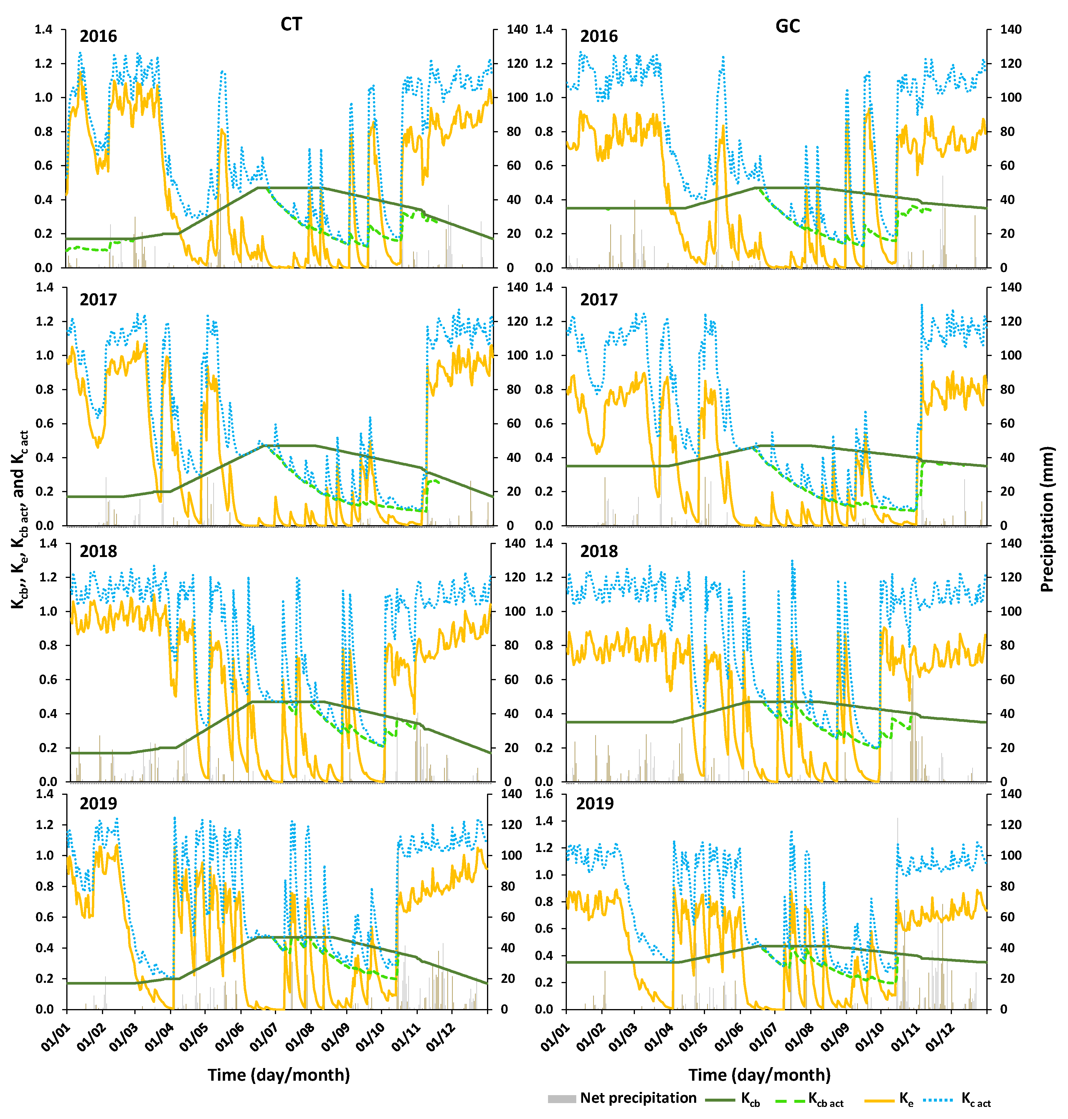
3.1. Model Parametrization

Table 5 presents the model parameters calibrated for the Italian and Portuguese plots with data relative to 2019 and 2020, respectively. These parameters were then validated for 2016–2018 relative to the Monferrato vineyards and for 2017 and 2019 relative to the Samora Correia vineyard. The initial Kcb values were obtained from tabulated data provided by Pereira et al. [56]. For Monferrato vineyards in year 2019, the calibrated Kcb ini, Kcb mid, and Kcb end values were, respectively, 0.20, 0.47, and 0.34 in the conventional tillage CT plot, and, respectively, 0.35, 0.47, and 0.40 in the ground cover GC plot. The active ground cover promoted an increase of the Kcb values in the initial and end season, while no differences were noticed in the mid-season. During this period, the inter-row grass was at the end of its annual cycle or already dried out. In the Samora Correia plot in year 2020, the calibrated Kcb ini, Kcb mid, and Kcb end were 0.17, 0.47, and 0.39, with the same Kcb mid as in Monferrato but with different Kcb ini and Kcb end.
Vineyards are heterogeneous, sparsely vegetated surfaces with complex canopies. For that, the Kcb values may vary among locations due to differences in varieties, age, training, irrigation, soil cover, and crop management as demonstrated in the recent literature review by Rallo et al. [53]. These authors updated the Kcb values proposed by Allen et al. [54] for vines and other perennial crops. Rallo et al. [53] provided standard Kcb for diverse training systems used in vineyards combined with the fraction of the ground cover (fc) but not including active ground cover calculations. After reviewing literature relative to wine grapes, it was concluded that for the training system adopted in the all the studied vineyards (vertical shoot positioned trellis), the fc values were reported to vary from 0.25 to 0.45, with Kcb mid values ranging from 0.46 to 0.80 and Kcb end values varying from 0.20 to 0.60. The Kcb values in both Monferrato and Samora Correia vineyards were therefore close to the lower limit of the range of variation of VSP trained vineyards reported by Rallo et al. [53]. The fc values observed during the mid-season stage in the Monferrato CT plot (0.35−0.39) and in the GC plot (0.25–0.29), as well as in the Samora Correia plot (0.35−0.36) (Table 4) were closer to the lower fc values reported by Rallo et al. [53], hence indicating that it is likely that the low Kcb mid and Kcb end values found in the current study are due to a small fc observed in the vineyards under study, so in agreement with reported data of those authors.
The calibrated Kcb values listed in Table 5 correspond to the entire vineyard system (vine plants + active ground cover). Table 6 shows the partitions of those values based on formulations given in Section 2.3 and crop density data (fc and h) given in Table 4 for each crop stage and growing season. Contribution of the active ground cover to the Kcb value was obviously higher in the Monferrato GC plot, but the Kcb values of vine plants were smaller, especially during the mid and end season stages since, as explained earlier, the cover crop may influence plant’s vigor and reduce canopy leaf area and Tc act rates of the grapevine in the earlier development stages which will then also affect the mid-season period. When looking at the partition of the Kcb values, it becomes also the higher Kcb mid value at Samora Correia (Portugal), resulting from higher air temperature registered in that location.
The calibrated pini, pmid, and pend values (Table 5) matched those proposed by Allen et al. [54] in the Monferrato CT plot but were slightly smaller in the Monferrato GC and the Samora Correia vineyard. The GC plot showed the lowest p values, likely due to the competition for water by the active ground cover.
The Ze, TEW, and REW, as well as the aD and bD calibrated values reflect the hydraulic properties of the soils of the studied vineyards, a loamy sand to sandy textured soil in Samora Correia vs. a clay to clay-loam soils at Monferrato. Lastly, the CN values were set to 70 and 55 in Monferrato CT and GC plots, respectively, with the inter-row grass cover clearly impacting the calibrated values of CN. Those values are lower than the CN reported by Gaudin et al. [84] from an analysis of three runoff events (CN = 82) for a bare soil. For olive orchards, Romero et al [85] reported CN = 89 for bare soil, CN = 82 and 70 for well-established cover crop strips with, respectively, 1 and 3 m wide, and CN = 88 and 87 for degraded cover crop strips with the same widths. For the Samora Correia vineyard, where runoff is less relevant due to the flat topography, the CN = 65 value is, as expected, smaller. Romero et al. [85] pointed out the need for improvements in the SCS-CN method aiming at a better understanding of the effects of soil management practices on runoff formation. As shown in Biddoccu et al. [7], different soil management implementations for the same treatment can lead to high variability in the soil roughness and coverage (namely the RUSLE C-factor), for the same region or among different countries.

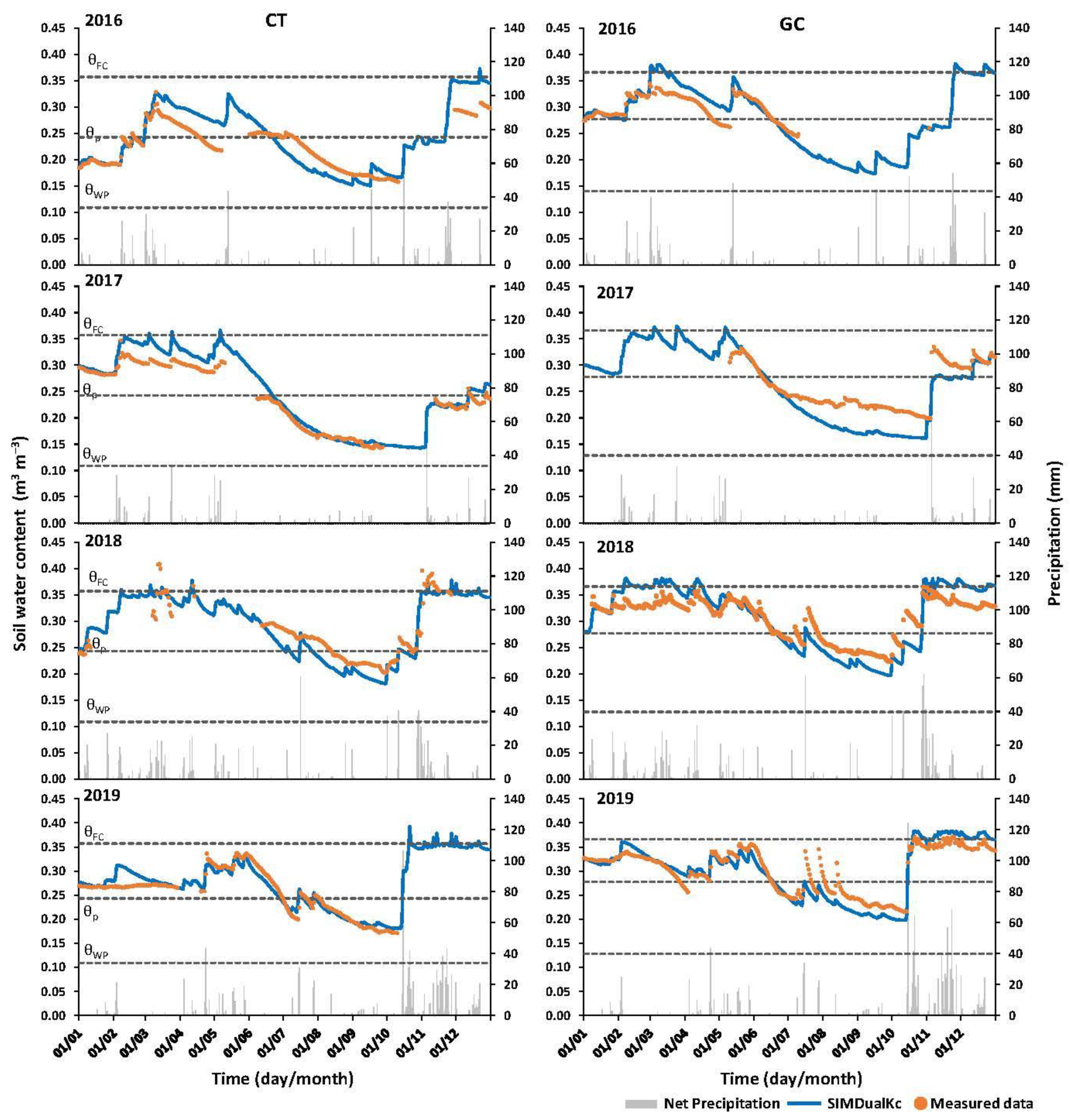
3.2. Model Performance

Figure 3 compares the SIMDualKc simulated soil water content (SWC) values in the root zone with daily measured SWC of Monferrato CT and GC plots during the years 2016–2019. Likewise, Figure 4 shows the measured and simulated SWC in the root zone of the Samora Correia vineyard during 2018–2020. Both figures further provide the dates and depths of rainfall events and, for the Portuguese vineyard, also of the irrigation dates and depths. Both figures show that the measured values of SWC were kept between θFC and θp during most of the year. In Monferrato, this fact resulted from precipitation, with large or successive events occurring during the autumn and spring, leading to SWC values temporarily above θFC. However, in the summer dry season, the soil moisture dropped below θp for some extended periods when rainfall was lacking. The year 2017 had the lowest SWC values as annual precipitation was uncharacteristically low during that year, amounting to only 493 mm. Indeed, among the last 20 years, 2017 was the least rainy one, with only 56% of the mean annual precipitation, while summer was very dry, with less than 25 mm of precipitation from the beginning of June to the end of August (the average for this period in 20 years is about 100 mm).
Simulated SWC were higher in GC plot relative to CT for all years, in agreement with the average of measured values. Likely, this would result from higher infiltration of rainfall water as already observed [5,11,12]. Nevertheless, Novara et al. [14], relative to a review of studies about the effects of a cover crop on SWC, reported that such effects often result in a decrease of soil moisture at a soil depth from 0–0.5 to 0–1.0 m, i.e., below the roots of the grass crop, between bloom and veraison, which can threaten yields in semiarid conditions.
In Samora Correia (Figure 4), drip irrigation was commonly applied at small depths (up to 12 mm) aimed at maintaining SWC above θp during the summer dry season. This type of irrigation management is uncommon in Portuguese vineyards of southern Portugal, where deficit irrigation is usually practiced during the summer dry period to better control shoot vigor and ripening, as well as the quality of fruit attributes [86,87]. Thus, the case observed at Samora Correia is rare and likely results from the very low water holding capacity of the soil, which calls the growers to avoid SWC < θp, at least during somewhat large periods.
The statistical indicators used to evaluate the agreement between measured and simulated SWC values are presented in Table 7 for both case studies. The SIMDualKc model performed well when simulating SWC in the Monferrato plots for calibration and for validation. The regression coefficient b0 varied from 0.95 to 1.06 in the CT plot and from 0.91 to 1.03 in the GC plot, i.e., close to the 1.0 target indicating that simulated values are close to the observed ones. The value of R2 was relatively high in both plots (0.76 to 0.90), showing that the model could explain most of the variability of the observed data. The errors of the estimates were small, resulting in a RMSE value ranging from 0.01 to 0.03 m3 m−3 and a NRMSE value ranging between 0.32 and 0.81. In agreement with b0, the PBIAS were small, not expressing a particular over- or under-estimation trend in simulating the measured data. The EF values were higher for CT than for GC (respectively, 0.53 to 0.90 and 0.34 to 0.80), indicating that the variance of the residuals was smaller than the measured data variance particularly for the calibration set. The goodness-of-fit indicators show better results for the CT plot relative to the GC case. This indicate that a supplemental effort for characterizing the active ground cover of the GC plots is required. Nevertheless, results obtained are reasonable enough for the pretended analysis.
The performance of the SIMDualKc model during the calibration period (2018) for the Samora Correia vineyard was comparable to results in the Italian case studies, with the PBIAS values, close to zero, also indicating accuracy in predicting the measured SWC. The regression coefficient b0 varied 1.00 to 1.02, thus leading to assume that there is no noticeable trends in the simulation, which is confirmed by the data. However, both the R2 and EF values are not high, indicating that improvements in describing vineyards crop data are required, particularly relative to the ground cover that changes from active to dry residues. The errors of the estimate RMSE were small, but the NRMSE are high because soil water depletion by evapotranspiration are low.
Issues related to the quality of the measured dataset and the empirical one-dimensional modeling approach used here to describe the soil water balance in a three-dimensional drip irrigation system may also help explaining why the goodness-of-fit indicators are not as high as in former studies, e.g., Paço et al. [88]. Nevertheless, the reported goodness-of-fit indicators are within the range of values reported in the literature for soil water content simulations of field crops [89,90], vegetable crops [91,92], and perennial crops [58,59,60,61] using the same model.

3.3. Soil Water Balance in the Hillslope Vineyards of Monferrato, Northern Italy

In Figure 5 are presented the daily values of the potential non-stressed basal crop coefficients (Kcb), the actual basal crop coefficients (Kcb act), the soil evaporation coefficients (Ke), and the actual crop coefficients (Kc act = Kcb act + Ke) computed by SIMDualKc. The rainfall events are also depicted in Figure 5. Table 8 presents then the components of the soil water balance in the Monferrato plots from 2016 to 2019.
The Kcb act matched the Kcb values during most of crop season duration except for the dry summers (Figure 5). The resulting seasonal Tc act values were estimated to vary from 262 to 313 mm in the CT plot and 298 to 339 mm in the GC plot (Table 8). Tc act values were up to 14% higher in the GC plot because comprising the transpiration by the grass cover in the inter-row. The Tc act reduction due to water stress started during mid-season and extended to the late-season due to low soil water availability during these dry months. The Tc act/Tc ratios are always smaller during the late season (Table 9) and the lowest value was observed in the late season of 2017 (0.30) due to the exceptional lack of rainfall in this year. Model results even suggested the need for irrigation in such dry conditions despite northern Italy is a traditionally rainfed wine-growing region. The impact of water stress on transpiration rates as given by the Tc act/Tc ratio was quite similar in both CT and GC plots with a general ratio value slightly smaller in the GC plot over three out of the four seasons. Despite the computed difference is small, it is noticeable in both the mid- and late-seasons, which explains the reluctance of winegrowers in using active ground cover in the inter-row due to concerns over soil water competition between the vines and the grass cover.
Table 9 further shows the Tc act values relative to the active ground cover (Tc act gcover). In the GC plot, the weight of Tc act gcover relative to Tc act of the entire vineyard system was always high, amounting to a maximum of 63.6% to 77.3% of the Tc act during the non-growing periods and to a minimum of 17.2% to 40.7% in the mid-season. In the CT plot, the ratios Tc act gcover/Tc act were naturally always smaller than those reported for the GC plot. It should be noticed that the fc values for the vineyard in the GC plot were always slightly lower than those in the CT plot (Table 4), which further exacerbates the importance of the cover crop to the soil water balance and preservation of soil and water resources in these hillslope areas.
The Ke values reached their maximum with the increase of soil moisture in the soil surface layer after rainfall events, rapidly decreasing in the following days as the soil dried out (Figure 5). For this reason, the Ke values have an enormous variability throughout the time. Es values were relatively similar in the GC and CT plots, with the small differences resulting from the different Ze set during calibration. The number of rainfall events influencing soil evaporation in each growing season is highly varied. Es values in the CT plot varied from 206 to 307 mm while in the GC plot they varied from 203 to 306 mm. Soil evaporation occurred mostly during the non-growing periods and early crop stages (Table 9) and was slightly larger in the CT plot because a fraction of the potential Es was used for ground cover transpiration.
In the CT plot, the seasonal simulated surface runoff ranged from 8 mm in 2017 to 355 mm in 2019. These values contrast with those estimated for the GC plot, which varied from 2 to 198 mm, i.e., 44% to 75% lower than in the CT plot. As shown in Figure 6, which compares the simulated and measured seasonal surface runoff in both plots during 2016–2019, the model provided a narrower range of runoff values when compared to field measurements. However, differences between CT and GC were well noticed. Computing runoff using a single CN value led the model to underestimate measured values during rainy years and overestimate them during drier seasons. Similarly, Celette et al. [48], when modelling the water balance in vineyards, observed that the use of a constant CN value for the surface runoff could not consider changes in the soil surface and their effects on runoff and water infiltration. Nevertheless, the SIMDualKc was able to catch the seasonal trends as well as the effect of inter-row management on runoff since measured values in the GC plot were also 50% to 78% lower than in the CT plot, thus very similar to the trend in model predictions. The model results are also in line with results of previous studies about cover crop and water conservation in olive orchards and vineyards in the Mediterranean area as reviewed by Novara et al. [14]. These authors showed that, on average, the annual runoff coefficient was reduced by 27% with the application of cover crop management. However, its effect on water conservation was higher in rainier regions (rainfall higher than 700 mm), whereas in drier regions it was not relevant. In sloping vineyards, the grass cover results not only in a reduction of runoff, but it contributes to decreasing significantly soil losses, up to 74% during very intense and erosive events [10,93]. On the one hand, improving the description of the soil coverage, either with the CT or the GC conditions, should improve the input data to the model and, therefore, its simulation capability; on the other hand, it is likely that simulations capabilities of the model may be enhanced. Nevertheless, current results are satisfactory and support the interpretation of the differences in behavior of vineyards, namely aspects that relate with the conservation of soil and water resources.
Lastly, the estimated percolation summed 27 to 467 mm in the CT plot and 8 to 600 mm in the GC plot. Except for 2017, which results were uncommon due to the very low precipitation, percolation was always higher 1.6% to 337% in the GC plot, with the grassed inter-row promoting higher infiltration rates, less runoff and soil erosion, thus higher groundwater recharge. Through direct measurements in vineyards of Montpellier, also with Mediterranean climate, Gaudin et al. [84] also observed that the presence of a permanent cover crop had a positive effect on water infiltration, favoring the refilling of the soil water profile. In any case, they observed that the soil water refilling at budbreak time was subjected to the rainfall pattern during the fall season.

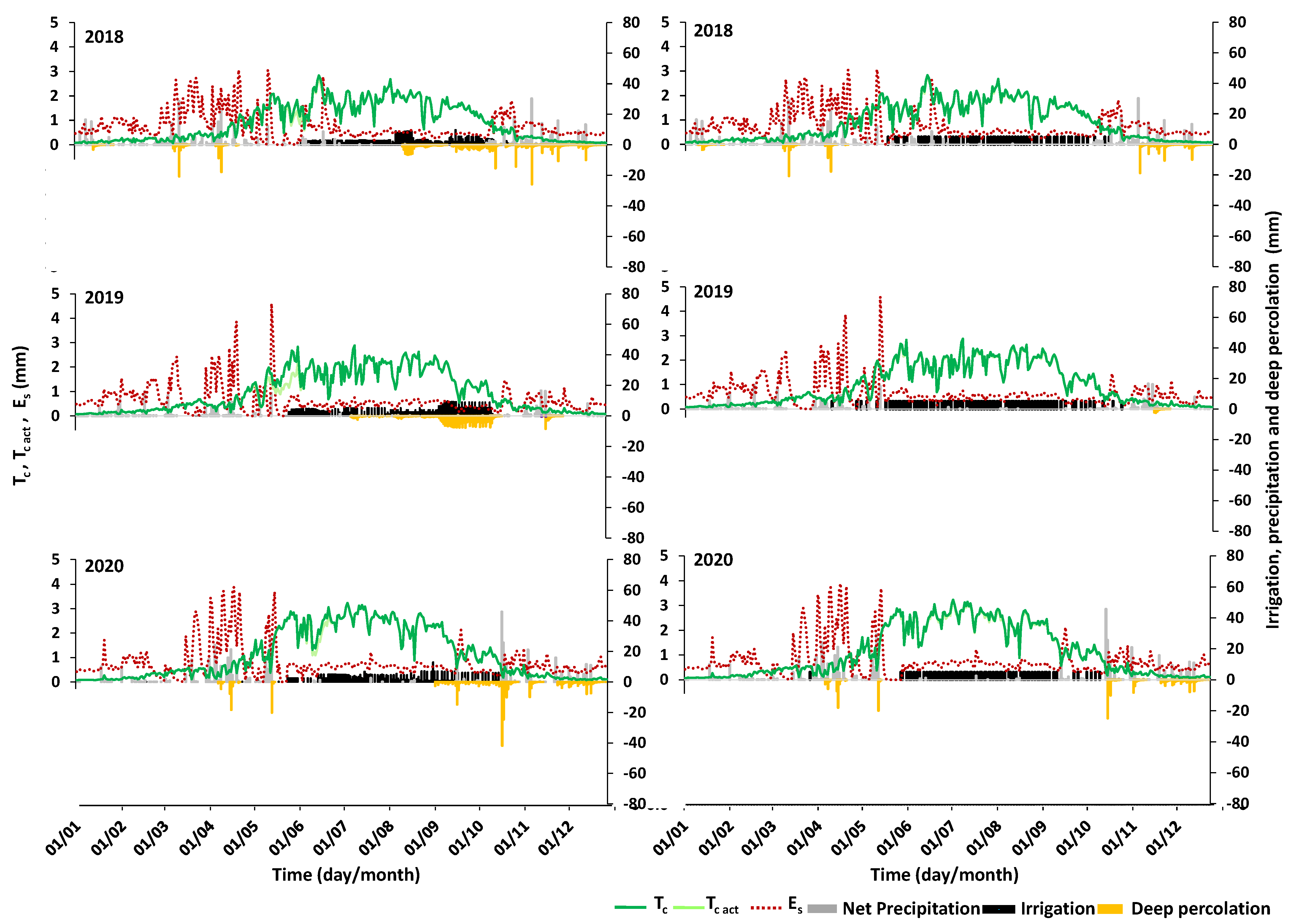
3.4. Soil Water Balance in the Irrigated Vineyard of Samora Correia, Southern Portugal

Figure 7 presents the daily values of the Kcb, Kcb act, Ke, and Kc act computed with the SIMDualKc for the years of 2018–2020. Rainfall and irrigation events are also depicted. The Kcb act matched the Kcb values throughout the growing seasons, meaning that the Tc act was always close to its potential values during the different stages of crop development as shown by the Tc act/Tc ratio always close to 1.0 in Table 10. The exception was only a small period during the rapid growth stage of the 2018 growing season where mild water stress was noticed. Irrigation was fundamental for such results, which otherwise would lead to a reduction of the Tc act values due to the high atmospheric demand observed particularly during the mid- and late season stages. The cover crop had only a small impact on Tc act values, with Tc act gcover being only expressive during the non-growing period (Table 11).
Like in the Italian case study, the Ke values reached their maximum after rainfall events, to then drop with the depletion of the evaporation soil layer. During the irrigation season, Ke values were maintained at a much lower range, close to 0.2 (Figure 7), resulting from the low fw value (0.13) describing evaporation from a small wetting bulb around emitters as opposite to rainfall events where the entire soil surface is wetted, and soil evaporation is maximized. The seasonal Es values then ranged from 235 to 281 mm (Table 10), corresponding to 40% to 45% of the ETc, and were distributed in relatively similar proportions throughout the different crop stages (Table 11).
The computed percolation was high, with values varying from 265 to 342 mm in the considered years (Table 10) which relates with the high infiltration and hydraulic conductivity of the sandy soil. In 2020, 23% (65 mm) of the seasonal percolation resulted from irrigation excess, corresponding to 14% of the water applied. In contrast, in 2019, seasonal percolation resulted mostly from irrigation surplus (92%; 243 mm), mainly during the late season, which corresponded to 39% of the total water applied through irrigation. These findings evidence the need for improving irrigation management in the considered field. Therefore, an optimization of irrigation schedules was considered by setting irrigation depths to 5 mm and the management allowed depletion (MAD) equal to the depletion fraction for no stress (p). This application revealed a substantial reduction of percolation losses during the monitored seasons without affecting the remaining components of the soil water balance (Table 10). This is visible in Figure 8, which compares the daily values of the different components of the soil water balance monitored in the field with those computed by the model when optimizing the irrigation schedules. Nonetheless, irrigation water management in vineyards is relatively more complex than the analysis shown herein since impacts on fruit quality are not considered. Hence, in future studies, it would be of interest to relate the SIMDualKc simulated irrigation schedules with both grapes yield and main characteristics of fruit quality for a better understanding of the impacts of irrigation management on crop development and yields.

4. Conclusions

This paper presents two study cases, one at Monferrato, northern Italy, analyzing alternative soil management issues, conventional tillage (CT) and grass cover (GC) as active ground cover, the other at Samora Correia, southern Portugal, drip irrigated. The vineyards are cultivated in different climates, humid at Monferrato, where soils have a large water holding capacity, and dry subhumid at Samora Correia, where the soil is sandy and therefore has a small water holding capacity. The SIMDualKc model was successful used for both cases to simulate water use (crop evapotranspiration) and the soil water balance. The model was calibrated and validated using, respectively, 4 and 3 years of soil moisture measurements, thus making it able to simulate soil and water management conditions observed in northern Italy and southern Portugal case studies.
The SIMDualKc model, adopting the dual Kc approach, was able to partitioning crop evapotranspiration into transpiration and evaporation from the soil. Moreover, it was able to compute distinctively the transpiration from the vine plants and the active ground cover. Results are satisfactory but it was observed that a better description of both the active ground cover and the mulch residues resulting from drying the former in summer is required, as well as improving related model simulation.
The Kcb values estimated over the different crop stages in the plot having the inter-row grass cover (GC) were higher than in the tilled CT plot, indicating higher transpiration of both the vines and the grass cover. The use of grass cover in the inter-row did not affect the ratio between the actual and potential root water uptake rates, i.e., the cover crop did not cause additional water stress to the grapevine except in conditions of great weather dryness of a peculiar year. On the contrary, the cover crop promoted infiltration of surface water and groundwater recharge, thus decreasing the risk of soil erosion and land degradation in addition to increase soil water availability, which confirmed previous studies reported in literature. Adopting the SIMDualKc model may support further analysis of problems and respective issues for improvement. Long term economic gains for adopting active ground cover are important relative to resource conservation, water and soil, due to controlling runoff and erosion with small increases in water stress. Nevertheless, financial gains in the short term are likely small, which limits active ground cover adoption by growers. Thus, it is adequate to search innovative approaches to adopt an active ground cover in the inter-rows, including searching the most adequate grass to be used, as well as with better consideration of the impacts of field slopes, always focusing both the soil and water conservation and the economic and financial return of farming.
Relative to the drip irrigation of sandy soils, the computed components of the soil water balance evidenced the need for improving irrigation management, mainly irrigation schedules, and the drip irrigation design, despite not dealt in the current study but known as limiting the performance of the irrigation system. In fact, crop transpiration needs to be increased relative to the total water use, which refers to increase the wetted bulbs to favor roots development and water extraction from the soil in combination with controlling percolation losses, so also favoring resource conservation. Using SIMDualKc as a decision support system should be appropriate.

Author Contributions

Conceptualization, M.B. and T.B.R.; methodology, T.B.R.; software, H.D. and L.S.P.; validation, T.B.R., H.D. and M.B.; formal analysis, T.B.R. and E.C.; investigation, T.B.R., L.S., G.C. and G.B.; resources, D.R., M.B., E.C. and T.B.R.; data curation, G.C.; writing—original draft preparation, T.B.R., H.D. and M.B.; writing—review and editing, D.R., G.B. and L.S.; visualization, G.C. and G.B.; supervision, M.B. and L.S.; project administration, M.B. and T.B.R.; funding acquisition, D.R., M.B., E.C. and T.B.R. All authors have read and agreed to the published version of the manuscript.

Funding

This research was carried out within the framework of the WATER4EVER Project (WaterJPI/0010/2016), which is funded under the WaterWorks 2015 Call, with the contribution of EU, FCT, and MIUR (Ministero per l’Istruzione, l’Università e la Ricerca), contract agreement WaterJPI/0010/2016. T.B. Ramos and H. Darouich were supported by contracts CEECIND/01152/2017 and CEECIND/01153/2017, respectively, from the Portuguese Fundação para a Ciência e a Tecnologia (FCT).

Data Availability Statement

Data available in a publicly accessible repository that does not issue DOIs. Publicly available datasets were analyzed in this study. This data can be found here: https://ismn.geo.tuwien.ac.at/en/ (last accessed on 30 March 2020).

Acknowledgments

Authors thank the support of Paula Paredes in using the model.

Conflicts of Interest

The authors declare no conflict of interest.

References

  1. Corti, G.; Cavallo, E.; Cocco, S.; Biddoccu, M.; Brecciaroli, G.; Agnelli, A. Evaluation of Erosion Intensity and Some of Its Consequences in Vineyards from Two Hilly Environments Under a Mediterranean Type of Climate, Italy. In Soil Erosion Issues in Agriculture; Godone, D., Stanchi, S., Eds.; InTechOpen: London, UK, 2011; pp. 113–160. [Google Scholar]
  2. Aguilera, E.; Lassaletta, L.; Gattinger, A.; Gimeno, B.S. Managing soil carbon for climate change mitigation and adaptation in Mediterranean cropping systems: A meta-analysis. Agr. Ecosyst. Environ. 2013, 168, 25–36. [Google Scholar] [CrossRef]
  3. Foronda-Robles, C. The territorial redefinition of the Vineyard Landscape in the sherry wine region (Spain). Misc. Geogr. 2018, 22, 95–101. [Google Scholar] [CrossRef] [Green Version]
  4. UNESCO. Vineyard Landscape of Piedmont: Langhe-Roero and Monferrato. 2021. Available online: http://whc.unesco.org/en/list/1390 (accessed on 17 December 2021).
  5. Salomé, C.; Coll, P.; Lardo, E.; Metay, A.; Villenave, C.; Marsden, C.; Blanchart, E.; Hinsinger, P.; Le Cadre, E. The soil quality concept as a framework to assess management practices in vulnerable agroecosystems: A case study in Mediterranean vineyards. Ecol. Indic. 2016, 61, 456–465. [Google Scholar] [CrossRef]
  6. Biddoccu, M.; Opsi, F.; Cavallo, E. Relationship between runoff and soil losses with rainfall characteristics and long-term soil management practices in a hilly vineyard (Piedmont, NW Italy). Soil Sci. Plant Nutr. 2014, 60, 92–99. [Google Scholar] [CrossRef] [Green Version]
  7. Biddoccu, M.; Guzman, G.; Capello, G.; Thielke, T.; Strauss, P.; Winter, S.; Zaller, J.G.; Nicolai, A.; Cluzeau, D.; Popescu, D.; et al. Evaluation of soil erosion risk and identification of soil cover and management factor (C) for RUSLE in European vineyards with different soil management. Int. Soil Water Conserv. Res. 2020, 8, 337–353. [Google Scholar] [CrossRef]
  8. Gómez, J.A.; Llewellyn, C.; Basch, G.; Sutton, P.B.; Dyson, J.S.; Jones, C.A. The effects of cover crops and conventional tillage on soil and runoff loss in vineyards and olive groves in several Mediterranean countries. Soil Use Manage. 2011, 27, 502–514. [Google Scholar] [CrossRef] [Green Version]
  9. Prosdocimi, M.; Cerdà, A.; Tarolli, P. Soil water erosion on Mediterranean vineyards: A review. Catena 2016, 141, 1–21. [Google Scholar] [CrossRef]
  10. Capello, G.; Biddoccu, M.; Cavallo, E. Permanent cover for soil and water conservation in mechanized vineyards: A study case in Piedmont, NW Italy. Ital. J. Agron. 2020, 15, 323–331. [Google Scholar] [CrossRef]
  11. Ruiz-Colmenero, M.; Bienes, R.; Marques, M.J. Soil and water conservation dilemmas associated with the use of green cover in steep vineyards. Soil Till. Res. 2011, 117, 211–223. [Google Scholar] [CrossRef]
  12. Napoli, M.; Dalla Marta, A.; Zanchi, C.A.; Orlandini, S. Assessment of soil and nutrient losses by runoff under different soil management practices in an Italian hilly vineyard. Soil Till. Res. 2017, 168, 71–80. [Google Scholar] [CrossRef]
  13. Medrano, H.; Tomás, M.; Martorell, S.; Escalona, J.-M.; Pou, A.; Fuentes, S.; Flexas, J.; Bota, J. Improving water use efficiency of vineyards in semi-arid regions. A review. Agron. Sustain. Dev. 2015, 35, 499–517. [Google Scholar] [CrossRef] [Green Version]
  14. Novara, A.; Cerda, A.; Barone, E.; Gristina, L. Cover crop management and water conservation in vineyard and olive orchards. Soil Till. Res. 2021, 208, 104896. [Google Scholar] [CrossRef]
  15. Pessina, D.; Galli, L.E.; Santoro, S.; Facchinetti, D. Sustainability of Machinery Traffic in Vineyard. Sustainability 2021, 13, 2475. [Google Scholar] [CrossRef]
  16. Bagagiolo, G.; Biddoccu, M.; Rabino, D.; Cavallo, E. Effects of rows arrangement, soil management, and rainfall characteristics on water and soil losses in Italian sloping vineyards. Environ. Res. 2018, 166, 690–704. [Google Scholar] [CrossRef]
  17. Rodrigo-Comino, J.; Senciales, J.M.; Ramos, M.A.; Martínez-Casasnovas, J.A.; Lasanta, T.; Brevik, E.C.; Ries, J.B.; Sinoga, J.R. Understanding soil erosion processes in Mediterranean sloping vineyards (Montes de Málaga, Spain). Geoderma 2017, 296, 47–59. [Google Scholar] [CrossRef] [Green Version]
  18. Keesstra, S.; Pereira, P.; Novara, A.; Brevik, E.C.; Azorin-Molina, C.; Parras-Alcántara, L.; Jordán, A.; Cerdà, A. Effects of soil management techniques on soil water erosion in apricot orchards. Sci. Total Environ. 2016, 551–552, 357–366. [Google Scholar] [CrossRef] [Green Version]
  19. Ben-Salem, N.; Álvarez, S.; López-Vicente, M. Soil and water conservation in rainfed vineyards with common sainfoin and spontaneous vegetation under different ground conditions. Water 2018, 10, 1058. [Google Scholar] [CrossRef] [Green Version]
  20. Garcia, L.; Celette, F.; Gary, C.; Ripoche, A.; Valdés-Gómez, H.; Metay, A. Management of service crops for the provision of ecosystem services in vineyards: A review. Agr. Ecosyst. Environ. 2018, 251, 158–170. [Google Scholar] [CrossRef] [Green Version]
  21. Winter, S.; Bauer, T.; Strauss, P.; Kratschmer, S.; Paredes, D.; Popescu, D.; Landa, B.; Guzmán, G.; Gómez, J.A.; Guernion, M.; et al. Effects of vegetation management intensity on biodiversity and ecosystem services in vineyards: A meta-analysis. J. Appl. Ecol. 2018, 55, 2484–2495. [Google Scholar] [CrossRef] [Green Version]
  22. Guzmán, G.; Cabezas, J.M.; Sánchez-Cuesta, R.; Lora, Á.; Bauer, T.; Strauss, P.; Winter, S.; Zaller, J.G.; Gómez, J.A. A field evaluation of the impact of temporary cover crops on soil properties and vegetation communities in southern Spain vineyards. Agr. Ecosyst. Environ. 2019, 272, 135–145. [Google Scholar] [CrossRef]
  23. Celette, F.; Gaudin, R.; Gary, C. Spatial and temporal changes to the water regime of a Mediterranean vineyard due to the adoption of cover cropping. Eur. J. Agron. 2008, 29, 153–162. [Google Scholar] [CrossRef]
  24. Ruiz-Colmenero, M.; Bienes, R.; Eldridge, D.J.; Marques, M.J. Vegetation cover reduces erosion and enhances soil organic carbon in a vineyard in the central Spain. Catena 2013, 104, 153–160. [Google Scholar] [CrossRef]
  25. Lopes, C.M.; Santos, T.P.; Monteiro, A.; Rodrigues, M.; Costa, J.M.; Chaves, M.M. Combining cover cropping with deficit irrigation in a Mediterranean low vigor vineyard. Sci. Hortic. 2011, 129, 603–612. [Google Scholar] [CrossRef] [Green Version]
  26. Williams, L.E.; Matthews, M.A. Grapevine. In Irrigation of Agricultural Crops; Agronomy Monographs No. 30. ASA-CSSA-SSSA; Stewart, B.J., Nielsen, D.R., Eds.; Agronomy Monographs: Madison, WI, USA, 1990; pp. 1019–1055. [Google Scholar]
  27. Costa, J.M.; Vaz, M.; Escalona, J.; Egipto, R.; Lopes, C.; Medrano, H.; Chaves, M.M. Modern viticulture in southern Europe: Vulnerabilities and strategies for adaptation to water scarcity. Agric. Water Manage. 2016, 164, 5–18. [Google Scholar] [CrossRef]
  28. Hannah, L.; Roehrdanz, P.R.; Ikegami, M.; Shepard, A.V.; Shaw, M.R.; Tabor, G.; Zhi, L.; Marquet, P.A.; Hijmans, R.J. Climate change, wine, and conservation. PNAS 2013, 110, 6907–6912. [Google Scholar] [CrossRef] [Green Version]
  29. Organisation Internationale de la Vigne et du Vin (OIV). State of the vitiviniculture world market 2021. 2021. Available online: https://www.oiv.int/en/technical-standards-and-documents/statistical-analysis/state-of-vitiviniculture (accessed on 17 December 2021).
  30. Zarrouk, O.; Francisco, R.; Pinto-Marijuan, M.; Brossa, R.; Santos, R.R.; Pinheiro, C.; Costa, J.M.; Lopes, C.; Chaves, M.M. Impact of irrigation regime on berry development and flavonoids composition in Aragonez (Syn. Tempranillo) grapevine. Agr. Water Manage. 2012, 114, 18–29. [Google Scholar] [CrossRef]
  31. Esteban, M.A.; Villanueva, M.J.; Lissarrague, J.R. Effect of irrigation on changes in the anthocyanin composition of the skin of cv Tempranillo (Vitis vinifera L) grape berries during ripening. J. Sci. Food Agr. 2001, 81, 409–420. [Google Scholar] [CrossRef]
  32. Permanhani, M.; Costa, J.M.; Conceição, M.A.F.; De Souza, R.T.; Vasconcellos, M.A.S.; Chaves, M.M. Deficit irrigation in table grape: Eco-physiological basis and potential use to save water and improve quality. Theor. Exp. Plant Phys. 2016, 28, 85–108. [Google Scholar] [CrossRef] [Green Version]
  33. Whitmore, A.P.; Schröder, J.J. Intercropping reduces nitrate leaching from under field crops without loss of yield: A modelling study. Eur. J. Agron. 2007, 27, 81–88. [Google Scholar] [CrossRef]
  34. Clothier, B.E.; Green, S.R. The leaching and runoff of nutrients from vineyards. In Science and Policy: Nutrient Management Challenges for the Next Generation; Occasional Report No. 30; Currie, L.D., Hedley, M.J., Eds.; Fertilizer and Lime Research Centre, Massey University: Palmerston North, New Zealand, 2017; 7p. [Google Scholar]
  35. Steenwerth, K.L.; Belina, K.M. Vineyard weed management practices influence nitrate leaching and nitrous oxide emissions. Agric. Ecosyst. Environ. 2010, 138, 127–131. [Google Scholar] [CrossRef]
  36. Andreoli, V.; Cassardo, C.; La Iacona, T.; Spanna, F. Description and preliminary simulations with the Italian vineyard integrated numerical model for estimating physiological values (IVINE). Agron. J. 2019, 9, 94. [Google Scholar] [CrossRef] [Green Version]
  37. Bagagiolo, G.; Rabino, D.; Biddoccu, M.; Nigrelli, G.; Cat Berro, D.; Mercalli, L.; Spanna, F.; Capello, G.; Cavallo, E. Effects of inter-annual climate variability on grape harvest timing in rainfed hilly vineyards of Piedmont (NW Italy). Ital. J. Agrometeorol. 2021, 1, 37–49. [Google Scholar] [CrossRef]
  38. Fraga, H.; De Cortázar Atauri, I.G.; Malheiro, A.C.; Moutinho-Pereira, J.; Santos, J.A. Viticulture in Portugal: A review of recent trends and climate change projections. Oeno One 2017, 51, 61–69. [Google Scholar] [CrossRef] [Green Version]
  39. Scherrer, S.C.; Begert, M.; Croci Maspoli, M.; Appenzeller, C. Long series of Swiss seasonal precipitation: Regionalization trends and influence of large scale flow. Int. J. Climatol. 2016, 36, 3673–3689. [Google Scholar] [CrossRef] [Green Version]
  40. Masson-Delmotte, V.; Zhai, P.; Pörtner, H.-O.; Roberts, D.; Skea, J.; Shukla, P.R.; Pirani, A.; Moufouma-Okia, W.; Péan, C.; Pidcock, R.; et al. Impacts of Global Warming of 1.5 °C above Pre-industrial Levels and Related Global Greenhouse Gas Emission Pathways, in the Context of Strengthening the Global Response to the Threat of Climate Change, Sustainable Development, and Efforts to Eradicate Poverty. Global Warming of 1.5 °C., an IPCC Special Report, IPCC. 2018. Available online: https://www.ipcc.ch/sr15/ (accessed on 17 December 2021).
  41. Allen, R.G.; Pereira, L.S.; Howell, T.A.; Jensen, M.E. Evapotranspiration information reporting: I. Factors governing measurement accuracy. Agric. Water Manag. 2011, 98, 899–920. [Google Scholar] [CrossRef] [Green Version]
  42. Pereira, L.S.; Paredes, P.; Jovanovic, N. Soil water balance models for determining crop water and irrigation requirements and irrigation scheduling focusing on the FAO56 method and the dual Kc approach. Agric. Water Manage. 2020, 241, 106357. [Google Scholar] [CrossRef]
  43. Pôças, I.; Gonçalves, J.; Costa, P.M.; Gonçalves, I.; Pereira, L.S.; Cunha, M. Hyperspectral-based predictive modelling of grapevine water status in the Portuguese Douro wine region. Int. J. Appl. Earth Observ. Geoinf. 2017, 58, 177–190. [Google Scholar] [CrossRef]
  44. Ortega-Farias, S.; Condori, W.E.; Riveros-Burgos, C.; Fuentes-Peñailillo, F.; Bardeen, M. Evaluation of a two-source patch model to estimate vineyard energy balance using high-resolution thermal images acquired by an unmanned aerial vehicle (UAV). Agric. For. Meteo. 2021, 304–305, 108433. [Google Scholar] [CrossRef]
  45. Romero, M.; Luo, Y.; Su, B.; Fuentes, S. Vineyard water status estimation using multispectral imagery from an UAV platform and machine learning algorithms for irrigation scheduling management. Comput. Electron. Agric. 2018, 147, 109–117. [Google Scholar] [CrossRef]
  46. Cancela, J.J.; Fandiño, M.; Rey, B.J.; Martinez, E.M. Automatic irrigation system based on dual crop coefficient, soil and plant water status for Vitis vinifera (cv Godello and cv Mencía). Agric. Water Manage. 2015, 151, 52–63. [Google Scholar] [CrossRef]
  47. Silva, S.P.; Valín, M.I.; Mendes, S.; Araujo-Paredes, C.; Cancela, J. Dual crop coefficient approach in Vitis vinifera L. cv. Loureiro. Agronomy 2021, 11, 2062. [Google Scholar] [CrossRef]
  48. Celette, F.; Ripoche, A.; Gary, C. WaLIS—A simple model to simulate water partitioning in a crop association: The example of an intercropped vineyard. Agr. Water Manage. 2010, 97, 1749–1759. [Google Scholar] [CrossRef]
  49. Phogat, V.; Pitt, T.; Stevens, R.M.; Cox, J.W.; Šimůnek, J.; Petrie, P.R. Assessing the role of rainfall redirection techniques for arresting the land degradation under drip irrigated grapevines. J. Hydrol. 2020, 587, 125000. [Google Scholar] [CrossRef]
  50. Kustas, W.P.; Alfieri, J.G.; Nieto, H.; Wilson, T.G.; Gao, F.; Anderson, M.C. Utility of the two-source energy balance (TSEB) model in vine and interrow flux partitioning over the growing season. Irrig. Sci. 2019, 37, 375–388. [Google Scholar] [CrossRef]
  51. Kool, D.; Kustas, W.P.; Ben-Gal, A.; Agam, N. Energy partitioning between plant canopy and soil, performance of the two-source energy balance model in a vineyard. Agr. For. Meteorol. 2021, 300, 108328. [Google Scholar] [CrossRef]
  52. Loddo, S.; Soccol, M.; Perra, A.; Ucchesu, M.; Meloni, P.; Barbaro, M.; Lo Cascio, M.; Sirca, C. Biosensing IoT platform for water management in vineyards. In Proceedings of the 2020 IEEE International Symposium on Circuits and Systems (ISCAS), Seville, Spain, 12–14 October 2020. [Google Scholar] [CrossRef]
  53. Rallo, G.; Paço, T.A.; Paredes, P.; Puig-Sirera, À.; Massai, R.; Provenzano, G.; Pereira, L.S. Updated single and dual crop coefficients for tree and vine fruit crops. Agric. Water Manage. 2021, 250, 106645. [Google Scholar] [CrossRef]
  54. Allen, R.G.; Pereira, L.S.; Raes, D.; Smith, M. Crop Evapotranspiration—Guidelines for Computing Crop Water Requirements; Irrigation & Drainage Paper 56; FAO: Rome, Italy, 1998. [Google Scholar]
  55. Allen, R.G.; Pereira, L.S.; Smith, M.; Raes, D.; Wright, J.L. FAO-56 dual crop coefficient method for estimating evaporation from soil and application extensions. J. Irrig. Drain. Eng. 2005, 131, 2–13. [Google Scholar] [CrossRef] [Green Version]
  56. Pereira, L.S.; Paredes, P.; Melton, F.; Johnson, L.; Mota, M.; Wang, T. Prediction of crop coefficients from fraction of ground cover and height: Pratical application to vegetable, field, and fruit crops with focus on parameterization. Agric. Water Manage. 2021, 252, 106663. [Google Scholar] [CrossRef]
  57. Rosa, R.D.; Paredes, P.; Rodrigues, G.C.; Alves, I.; Fernando, R.M.; Pereira, L.S.; Allen, R.G. Implementing the dual crop coefficient approach in interactive software. 1. Background and computational strategy. Agric. Water Manage. 2012, 103, 8–24. [Google Scholar] [CrossRef]
  58. Fandiño, M.; Cancela, J.J.; Rey, B.J.; Martínez, E.M.; Rosa, R.G.; Pereira, L. Using the dual-Kc approach to model evapotranspiration of Albariño vineyards (Vitis vinifera L. cv. Albariño) with consideration of active ground cover. Agric. Water Manage. 2012, 112, 75–87. [Google Scholar] [CrossRef]
  59. Paço, T.; Ferreira, M.; Rosa, R.; Paredes, P.; Rodrigues, G.; Conceição, N.; Pacheco, C.; Pereira, L. The dual crop coefficient approach using a density factor to simulate the evapotranspiration of a peach orchard: SIMDualKc model versus eddy covariance measurements. Irrig. Sci. 2012, 30, 115–126. [Google Scholar] [CrossRef]
  60. Paço, T.A.; Pôças, I.; Cunha, M.; Silvestre, J.C.; Santos, F.L.; Paredes, P.; Pereira, L.S. Evapotranspiration and crop coefficients for a super intensive olive orchard. An application of SIMDualKc and METRIC models using ground and satellite observations. J. Hydrol. 2014, 519, 2067–2080. [Google Scholar] [CrossRef] [Green Version]
  61. Puig-Sirera, À.; Rallo, G.; Paredes, P.; Paço, T.A.; Minacapilli, M.; Provenzano, G.; Pereira, L.S.S. Transpiration and water use of an irrigated traditional olive grove with Sap-Flow observations and the FAO56 dual crop coefficient approach. Water 2021, 13, 2466. [Google Scholar] [CrossRef]
  62. Biancotti, A.; Bellardone, G.; Bovo, S.; Cagnazzi, B.; Giacomelli, L.; Marchisio, C. Distribuzione Regionale di Piogge e Temperature. Collana Studi Climatologici del Piemonte, Vol.1; Regione Piemonte: Torino, Italy, 1998. [Google Scholar]
  63. Servizio Geologico Italiano. Carta Geologica d’Italia alla scala 1:100.000. 1969. Available online: http://193.206.192.231/carta_geologica_italia/cartageologica.htm (accessed on 17 December 2021).
  64. IUSS Working Group. World Reference Base for Soil Resources 2014: International Soil Classification System for Naming Soils and Creating Legends for Soil Maps; World Soil Resources Reports No. 106; Food and Agriculture Organization of the United Nations (FAO): Rome, Italy, 2014. [Google Scholar]
  65. Blake, G.R.; Hartge, K.H. Bulk density. In Methods of Soil Analysis. Part 1. Physical and Mineralogical Methods, 2nd ed.; Klute, A., Ed.; American Society of Agronomy–Soil Science Society of America: Madison, WI, USA, 1986; pp. 363–375. [Google Scholar]
  66. Cavazza, L. Fisica del Terreno Agrario. UTET: Torino, Italy, 1981. [Google Scholar]
  67. Schaap, M.G.; Leij, F.J.; van Genuchten, M.T. ROSETTA: A computer program for estimating soil hydraulic parameters with hierarchical pedotransfer functions. J. Hydrol. 2001, 251, 163–176. [Google Scholar] [CrossRef]
  68. Gomes, M.P.; Silva, A.A. Um novo diagrama triangular para a classificação básica da textura do solo. Garcia Orta 1962, 10, 171–179. [Google Scholar]
  69. Ramos, T.B.; Gonçalves, M.C.; Brito, D.; Martins, J.C.; Pereira, L.S. Development of class pedotransfer functions for integrating water retention properties into Portuguese soil maps. Soil Res. 2013, 51, 262–277. [Google Scholar] [CrossRef]
  70. Ramos, T.B.; Horta, A.; Gonçalves, M.C.; Martins, J.C.; Pereira, L.S. Development of ternary diagrams for estimating water retention properties using geostatistical approaches. Geoderma 2014, 230, 229–242. [Google Scholar] [CrossRef]
  71. ARPA Piemonte—Meteorologia e Clima. Available online: https://www.arpa.piemonte.it/dati-ambientali/dati-meteoidrografici-giornalieri-richiesta-automatica (accessed on 17 December 2021).
  72. Biddoccu, M.; Ferraris, S.; Opsi, F.; Cavallo, E. Long-term monitoring of soil management effects on runoff and soil erosion in sloping vineyards in Alto Monferrato (North–West Italy). Soil Till. Res. 2016, 155, 176–189. [Google Scholar] [CrossRef]
  73. Raffelli, G.; Previati, M.; Canone, D.; Gisolo, G.; Bevilacqua, I.; Capello, G.; Biddoccu, M.; Cavallo, E.; Deiana, R.; Cassiani, G.; et al. 2017. Local and plot-scale measurements of soil moisture: Time and spatially resolved field techniques in plain, hill and mountain sites. Water 2017, 9, 706. [Google Scholar] [CrossRef]
  74. Sohne, W. Druckverteilung im Boden und Boden-verformung unter Schlepper Reifen. Grundl. Der Landtech. 1953, 5, 49–63. [Google Scholar]
  75. Ritchie, J.T. Model for predicting evaporation from a row crop within complete cover. Water Resour. Res. 1972, 8, 1204–1213. [Google Scholar] [CrossRef] [Green Version]
  76. Liu, Y.; Pereira, L.S.; Fernando, R.M. Fluxes through the bottom boundary of the root zone in silty soils: Parametric approaches to estimate groundwater contribution and percolation. Agric. Water Manage. 2006, 84, 27–40. [Google Scholar] [CrossRef]
  77. USDA-SCS. National Engineering Handbook; Section 4, Table 10.1; 1972. Available online: https://directives.sc.egov.usda.gov/OpenNonWebContent.aspx?content=17752.wba (accessed on 17 December 2021).
  78. Allen, R.G.; Wright, J.L.; Pruitt, W.O.; Pereira, L.S.; Jensen, M.E. Water requirements. In Design and Operation of Farm Irrigation Systems, 2nd ed.; Hoffman, G.J., Evans, R.G., Jensen, M.E., Martin, D.L., Elliot, R.L., Eds.; ASABE: St. Joseph, MI, USA, 2007; pp. 208–288. [Google Scholar]
  79. Allen, R.G.; Pereira, L.S. Estimating crop coefficients from fraction of ground cover and height. Irrig. Sci. 2009, 28, 17–34. [Google Scholar] [CrossRef] [Green Version]
  80. Pereira, L.S.; Paredes, P.; Melton, F.; Johnson, L.; Wang, T.; López-Urrea, R.; Cancela, J.J.; Allen, R. Prediction of crop coefficients from fraction of ground cover and height. Background and validation using ground and remote sensing data. Agric. Water Manage. 2020, 240, 106197. [Google Scholar] [CrossRef]
  81. Pereira, L.S.; Paredes, P.; Rodrigues, G.C.; Neves, M. Modeling malt barley water use and evapotranspiration partitioning in two contrasting rainfall years. Assessing AquaCrop and SIMDualKc models. Agric. Water Manage. 2015, 159, 239–254. [Google Scholar] [CrossRef]
  82. Moriasi, D.N.; Arnold, J.G.; Van Liew, M.W.; Bingner, R.L.; Harmel, R.D.; Veith, T.L. Model Evaluation Guidelines for Systematic Quantification of Accuracy in Watershed Simulations. Trans. ASABE 2007, 50, 885–900. [Google Scholar] [CrossRef]
  83. Nash, J.E.; Sutcliffe, J.V. River flow forecasting through conceptual models part I—A discussion of principles. J. Hydrol. 1970, 10, 282–290. [Google Scholar] [CrossRef]
  84. Gaudin, R.; Celette, F.; Gary, C. Contribution of runoff to incomplete off season soil water refilling in a Mediterranean vineyard. Agric. Water Manage. 2010, 97, 1534–1540. [Google Scholar] [CrossRef]
  85. Romero, P.; Castro, G.; Gomez, J.A.; Fereres, E. Curve number values for olive orchards under different soil management. Soil Sci. Soc. Am. J. 2007, 71, 1758–1769. [Google Scholar] [CrossRef]
  86. Ferreira, M.I.; Silvestre, J.; Conceição, N.; Malheiro, A.C. Crop and stress coefficients in rainfed and deficit irrigation vineyards using sap flow techniques. Irrig. Sci. 2012, 30, 433–447. [Google Scholar] [CrossRef]
  87. Zarrouk, O.; Brunetti, C.; Egipto, R.; Pinheiro, C.; Genebra, T.; Gori, A.; Lopes, C.M.; Tattini, M.; Chaves, M.M. Grape ripening is regulated by deficit irrigation/elevated temperatures according to cluster position in the canopy. Front. Plant Sci. 2016, 7, 1640. [Google Scholar] [CrossRef] [Green Version]
  88. Paço, T.A.; Paredes, P.; Pereira, L.S.; Silvestre, J.; Santos, F.L. Crop Coefficients and Transpiration of a Super Intensive Arbequina Olive Orchard using the Dual Kc Approach and the Kcb Computation with the Fraction of Ground Cover and Height. Water 2019, 11, 383. [Google Scholar] [CrossRef] [Green Version]
  89. Paredes, P.; Rodrigues, G.C.; Alves, I.; Pereira, L.S. Partitioning evapotranspiration, yield prediction and economic returns of maize under various irrigation management strategies. Agric. Water Manage. 2014, 135, 27–39. [Google Scholar] [CrossRef]
  90. Rosa, R.D.; Ramos, T.B.; Pereira, L.S. The dual Kc approach to assess maize and sweet sorghum transpiration and soil evaporation under saline conditions: Application of the SIMDualKc model. Agric. Water Manage. 2016, 115, 291–310. [Google Scholar] [CrossRef]
  91. Darouich, H.; Karfoul, R.; Eid, H.; Ramos, T.B.; Baddour, N.; Moustafa, A.; Assaad, M.I. Modeling zucchini squash irrigation requirements in the Syrian Akkar region using the FAO56 dual-Kc approach. Agric Water Manage. 2020, 229, 105927. [Google Scholar] [CrossRef]
  92. Darouich, H.; Karfoul, R.; Ramos, T.B.; Moustafa, A.; Shaheen, B.; Pereira, L.S. Crop water requirements and crop coefficients for jute mallow (Corchorus olitorius L.) using the SIMDualKc model and assessing irrigation strategies for the Syrian Akkar region. Agric. Water Manage. 2021, 255, 107038. [Google Scholar] [CrossRef]
  93. Novara, A.; Cerdà, A.; Gristina, L. Sustainable vineyard floor management: An equilibrium between water consumption and soil conservation. Curr. Opin. Environ. Sci. Health. 2018, 5, 33–37. [Google Scholar] [CrossRef]
Figure 1. Weather data for Monferrato plots during the study period (P, precipitation, ETo, reference evapotranspiration; Tmax and Tmin, maximum and minimum air temperatures, RHavg, mean relative humidity; Rs, solar radiation, u2, wind speed at 2 m height).
Water 14 00554 g001
Figure 2. Weather data of Samora Correia case study (P, precipitation, ETo, reference evapotranspiration; Tmax and Tmin, maximum and minimum air temperatures; RHavg, mean relative humidity; Rs, solar radiation, u2, wind speed at 2 m height).
Water 14 00554 g002
Figure 3. Measured and simulated soil water contents of the Monferrato conventional tillage (CT) and grass cover (GC) plots during the 2016–2019 growing seasons (θFC, θWP, and θp refer to soil water contents at field capacity, the wilting point, and at the depletion fraction for no stress, respectively).
Water 14 00554 g003
Figure 4. Measured and simulated soil water contents in the vineyard of Samora Correia during the 2018–2020 growing seasons (θFC, θWP, and θp refer to soil water contents at field capacity, the wilting point, and at the depletion fraction for no stress, respectively).
Water 14 00554 g004
Figure 5. Seasonal evolution of the potential non-stressed basal crop coefficients (Kcb), the actual basal crop coefficients (Kcb act), the soil evaporation coefficients (Ke), and the actual crop coefficients (Kc act = Kcb act + Ke) computed by SIMDualKc for the Monferrato conventional tillage (CT) and grass cover (GC) plots during the 2016–2019 growing seasons.
Water 14 00554 g005
Figure 6. Simulated and measured seasonal runoff in the Monferrato plots with conventional tillage (CT) and grass cover (GC).
Water 14 00554 g006
Figure 7. Seasonal evolution of the potential non-stressed basal crop coefficients (Kcb), the actual basal crop coefficients (Kcb act), the soil evaporation coefficients (Ke), and the actual crop coefficients (Kc act = Kcb act + Ke) computed by SIMDualKc for the Samora Correia vineyard during the 2018–2020.
Water 14 00554 g007
Figure 8. Daily evolution of the potential crop transpiration (Tc), actual crop transpiration (Tc act), soil evaporation (Es), and deep percolation rates at Samora Correia vineyard as monitored in the field (left) and after optimization of the irrigation schedules (right) during 2018–2020.
Water 14 00554 g008
Table 1. Main soil physical characteristics in the different case studies (ρb, soil bulk density; θS, θFC, θWP, soil water contents at saturation, field capacity, and the wilting point, respectively; TAW, total available water).
Depth (cm)Soil Texture (%)ρb
(Mg m−3)
Soil Hydraulic Properties (m3 m−3)TAW
(mm)
Coarse Sand
(2000–200 μm)
Fine Sand
(200–20 μm)
Silt
(20–2 μm)
Clay
(<2 μm)
θSθFCθWP
Monferrato, Italy (conventional tillage plot)
0–1010.944.126.818.21.320.4370.3800.08329.7
10–2016.829.936.716.61.370.4430.3790.07830.1
20–3017.340.86.135.81.350.4360.3570.12723.0
30–10017.340.86.135.81.350.4360.3500.115164.5
Monferrato, Italy (grass cover plot)
0–1011.127.629.831.51.330.4530.3750.11526.0
10–209.527.330.432.81.320.4480.3980.11927.9
20–3013.828.426.831.01.280.4540.3720.11525.7
30–10013.828.426.831.01.280.4540.3500.135150.5
Samora Correia, Portugal
0–2059.726.89.44.11.680.4040.1780.06422.90
20–4060.126.09.44.41.650.4040.1780.06422.90
40–6063.325.97.53.31.720.4040.1450.04719.53
60–8072.219.45.52.8-0.3980.1100.03814.48
80–10079.614.24.41.8-0.3980.0940.02513.74
Table 2. Crop growth stage dates of vines in the various case studies and duration of growing seasons (in GDD).
Crop Growth Stages
YearNon-GrowingInitiationCrop
Development
Mid-
Season
Late-SeasonEnd-
Season
Non-GrowingTotal
GDD
Monferrato, northern Italy
201601/0112/0313/0413/0607/0831/1031/12
GDD-44325698684--1753
201701/0115/0330/0418/0601/0831/1031/12
GDD-123407582797--1910
201801/0118/0302/0407/0609/0831/1031/12
GDD-5391845742--1982
201901/0124/0308/0415/0619/0831/1031/12
GDD-20307897577--1801
Samora Correia, southern Portugal
201801/0113/0303/0425/0505/0815/1031/12
GDD-54308799904--2065
201901/0110/0313/0411/0613/0820/1031/12
GDD-150508700789--2147
202001/0125/0312/0431/0510/0823/1031/12
GDD-86423906822--2236
Note: GDD is the cumulative growing degree-days.
Table 3. Initial soil water contents in the root zone (% of TAW) and evaporable soil layer (% of TEW) in each case study and growing season.
Growing Season% of TAW% of TEW
Monferrato (CT)Monferrato (GC)S. CorreiaMonferrato (CT)Monferrato (GC)S. Correia
20166734-6734-
20172225-2225-
2018453330453330
2019311423311423
2020--17--17
Note: TAW, total available water; TEW, total evaporable water.
Table 4. Fraction of ground cover fc, crop height (h), fraction of the active ground cover (fc gcover) and height of the active ground cover (hgcover) in every plot and all growing seasons.
Monferrato (CT)Monferrato (GC)Samora Correia
VineyardInter-RowVineyardInter-RowVineyardInter-Row
fc
(-)
h
(m)
fc gcover
(-)
hgcover
(m)
fc
(-)
h
(m)
fc gcover
(-)
hgcover
(m)
fc
(-)
h
(m)
fc gcover
(-)
hgcover
(m)
2016
Non-Growing0.040.500. 200.200.050.500.820.18----
Initiation0.150.800.180.150.160.800.750.15----
Mid-season0.351.800.120.150.291.800.650.15----
Late-season0.271.200.180.150.231.200.770.15----
Non-Growing0.030.500.200.200.040.500.820.18----
2017
Non-Growing0.040.500. 200.200.030.500.810.18----
Initiation0.150.800.170.150.140.800.700.15----
Mid-season0.371.800.120.150.251.700.610.15----
Late-season0.281.200.180.150.231.100.720.15----
Non-Growing0.030.500.200.200.040.500.810.18----
2018
Non-Growing0.040.500.240.200.040.500.800.200.030.500.200.15
Initiation0.160.800.180.150.150.800.710.180.130.800.180.15
Mid-season0.371.900.130.150.291.800.590.170.361.700.070.10
Late-season0.301.200.260.150.221.200.740.180.301.200.180.10
Non-Growing0.030.500.260.200.040.500.800.200.040.500.200.15
2019
Non-Growing0.030.500.240.200.030.500.820.200.030.500.210.15
Initiation0.160.800.190.150.150.800.720.180.130.800.190.15
Mid-season0.391.900.130.150.291.800.600.180.351.700.080.10
Late-season0.301.200.250.150.221.200.750.180.291.200.180.10
Non-Growing0.030.500.250.200.040.500.820.200.030.500.200.15
2020
Non-Growing--------0.030.500.200.15
Initiation--------0.170.800.180.15
Mid-season--------0.361.700.080.10
Late-season--------0.311.200.180.10
Non-Growing--------0.030.500.200.15
Table 5. Default and calibrated model parameters.
ParametersUnitsDefault
Values
Calibrated Values
Monferrato
(CT)
Monferrato
(GC)
Samora Correia
Kcb nongrowing-0.150.170.350.16
Kcb ini-0.150.200.350.17
Kcb mid-0.650.470.470.47
Kcb end-0.400.340.400.39
pini-0.450.450.350.40
pmid-0.450.450.350.40
pend-0.450.450.350.40
TEWmm34–15303115
REWmm9–79117
Zem0.100.090.100.10
aDmm-360370152
bD-−0.0173−0.0150−0.0170−0.0173
CN-75–60705565
Note: CT, conventional tillage; GC, grass cover; Kcb, basal crop coefficient for the initial (Kcb ini), mid (Kcb mid), and end season (Kcb end); Kcb nongrowing, basal crop coefficient during the non-growing period; p, depletion fraction for no stress during the initial (pini), mid (pmid), and end season (pend); TEW, total evaporable water; REW, readily evaporable water; Ze, depth of the soil evaporation layer; aD and bD, parameters of the deep percolation; CN, curve number.
Table 6. Basal crop coefficient (Kcb) partitioning between the main crop (vine) and active ground cover (gcover) during the nongrowing season and at the initial, mid, end season crop stages.
ParametersMonferrato
(CT)
Monferrato
(GC)
Samora Correia
201620172018201920162017201820192018–2020
Kcb gcover nongrowing0.090.090.090.100.240.240.240.250.09
Kcb gcover ini0.080.080.080.080.220.210.220.230.08
Kcb gcover mid0.070.070.070.070.200.190.190.190.06
Kcb fcover end0.080.080.090.090.220.210.230.220.07
Kcb vine nongrowing0.090.090.100.100.240.240.240.240.09
Kcb vine ini0.120.120.120.120.130.140.130.120.09
Kcb vine mid0.400.400.400.400.270.280.280.280.41
Kcb vine end0.260.260.250.250.180.190.170.180.32
Table 7. Goodness-of-fit indicators for the adjustment between measured and simulated values in all case studies.
SiteYearTreatmentb0
(-)
R2
(-)
RMSE
(m3 m−3)
NRMSE
(-)
PBIAS
(%)
EF
(-)
Monferrato2016CT1.040.840.030.69−3.300.53
GC1.030.760.020.78−2.550.39
2017CT1.060.970.020.34−5.760.88
GC0.910.900.030.819.950.34
2018CT0.950.860.030.515.600.74
GC1.020.890.030.74−1.120.45
2019CT1.010.900.010.32−1.030.90
GC0.990.900.020.451.040.80
S. Correia2018-1.010.590.010.74−1.530.45
2019-1.020.570.010.86−1.840.30
2020-1.000.750.010.50−0.500.75
Note: b0, regression coefficient; R2, coefficient of determination; RMSE, root mean square error; NRMSE, ratio of the RMSE to the standard deviation of observed data; PBIAS, percent bias; NSE, model efficiency.
Table 8. Components of the soil water balance in the Monferrato plots.
YearPlot I
(mm)
P
(mm)
ΔSW
(mm)
Tc
(mm)
Tc act
(mm)
Es
(mm)
DP
(mm)
RO
(mm)
2016CT0779−1563722622342790
GC0779−8541729823411843
2017CT049335395275206428
GC0493−1744530020382
2018CT01190−100347313307310178
GC01189−8638632630631592
2019CT01476−68353313274467355
GC01476−40403339284600198
Note: I, irrigation; P, precipitation; ΔSW, soil water storage variation; Tc, potential transpiration; Tc act, actual transpiration; Es, evaporation; DP, deep percolation; RO, runoff.
Table 9. Evapotranspiration partitioning in the Monferrato vineyard plots during the different crop stages.
PeriodParameterUnits2016201720182019
CTGCCTGCCTGCCTGC
Non-GrowingTc act(mm)922132511212041
Tc act gcover(mm)5177176151229
Tc act/Tc(-)0.841.001.001.001.001.001.001.00
Es(mm)5850595261504847
Initial stageTc act(mm)152634526101017
Tc act gcover(mm)614112926411
Tc act/Tc(-)1.001.001.001.001.001.001.001.00
Es(mm)3737474822211110
Rapid growthTc act(mm)8599929972867994
Tc act gcover(mm)1830174416431747
Tc act/Tc(-)1.001.001.000.991.001.001.001.00
Es(mm)414539419495107111
Mid-seasonTc act(mm)98938572149135149132
Tc act gcover(mm)1516132922552253
Tc act/Tc(-)0.690.660.720.610.960.870.910.81
Es(mm)19217847545161
Late-seasonTc act(mm)4747444168624744
Tc act gcover(mm)8117181129820
Tc act/Tc(-)0.420.400.340.300.700.610.640.58
Es(mm)5258232758643032
Non-GrowingTc act(mm)711712711711
Tc act gcover(mm)18292728
Tc act/Tc(-)0.970.950.800.931.001.001.001.00
Es(mm)2623322824212623
TotalTc act(mm)262298275300313326313339
Tc act gcover(mm)5396571465915565168
Tc act/Tc(-)0.700.710.700.680.900.850.880.84
Es(mm)234234206203307306274284
Note: Tc, potential transpiration; Tc act, actual transpiration; Tc act gcover, actual transpiration of the active ground cover; Es, evaporation.
Table 10. Components of the soil water balance in the Samora Correia vineyard.
ScheduleYearI
(mm)
P
(mm)
ΔSW
(mm)
Tc
(mm)
Tc act
(mm)
Es
(mm)
DP
(mm)
RO
(mm)
Farmer2018454499−2832932427434213
2019625240−173503372352651
2020465506−134043992812837
Model2018295499−1932932727816913
2019375240−2335034723991
2020355506−144043992741707
Note: I, irrigation; P, precipitation; ΔSW, soil water storage variation; Tc, potential transpiration; Tc act, actual transpiration; Es, evaporation; DP, deep percolation; RO, runoff.
Table 11. Evapotranspiration partitioning in the Samora Correia vineyard during the different crop stages.
PeriodParameterUnits201820192020
Non-GrowingTc act(mm)121220
Tc act gcover(mm)6610
Tc act/Tc(-)1.001.001.00
Es(mm)586059
Initial stageTc act(mm)7167
Tc act gcover(mm)483
Tc act/Tc(-)1.001.001.00
Es(mm)332929
Vegetation growthTc act(mm)536669
Tc act gcover(mm)111414
Tc act/Tc(-)1.000.831.00
Es(mm)534759
Mid-seasonTc act(mm)122120173
Tc act gcover(mm)161522
Tc act/Tc(-)0.961.000.97
Es(mm)423045
Late-seasonTc act(mm)110106115
Tc act gcover(mm)212021
Tc act/Tc(-)1.001.001.00
Es(mm)333045
Non-GrowingTc act(mm)191715
Tc act gcover(mm)654
Tc act/Tc(-)1.001.001.00
Es(mm)554044
TotalTc act(mm)324337399
Tc act gcover(mm)636876
Tc act/Tc(-)0.990.960.99
Es(mm)274235281
Note: Tc, potential transpiration; Tc act, actual transpiration; Tc act gcover, actual transpiration of the active ground cover; Es, evaporation from the soil.
Publisher’s Note: MDPI stays neutral with regard to jurisdictional claims in published maps and institutional affiliations.

