Article

Modelling the Hydrological Effects of Woodland Planting on Infiltration and Peak Discharge Using HEC-HMS

1
Centre for Agroecology, Water and Resilience, Coventry University, Wolston Lane, Coventry CV8 3LG, UK
2
Faculty of Engineering, Environment & Computing, School of Energy, Construction and Environment, Coventry University, Coventry CV1 5FB, UK
3
IKT-Institute for Underground Infrastructure, Exterbruch 1, 45886 Gelsenkirchen, Germany
*
Author to whom correspondence should be addressed.
Water 2021, 13(21), 3039; https://doi.org/10.3390/w13213039
Submission received: 30 September 2021 / Revised: 19 October 2021 / Accepted: 26 October 2021 / Published: 31 October 2021
(This article belongs to the Special Issue Forms, Functions and Values of Treescapes (Natural and Urban))

Abstract

:
Woodland planting is gaining momentum as a potential method of natural flood management (NFM), due to its ability to break up soil and increase infiltration and water storage. In this study, a 2.2 km2 area in Warwickshire, England, planted with woodland every year from 2006 to 2012, was sampled using a Mini Disk infiltrometer (MDI). Infiltration measurements were taken from 10 and 200 cm away from the trees, from November 2019 to August 2021. Two individual hydrological models were built using the US Hydraulic Engineering Center Hydrological Modelling System (HEC-HMS), to model the effects of infiltration change on peak flows from the site throughout the summer and winter. The models were calibrated and validated using empirical data; the Nash and Sutcliffe Efficiency (NSE) was used as an indicator of accuracy. Results from this study show that woodland planting reduced peak flow intensity compared to impermeable land cover by an average of 6%, 2%, and 1% for 6-h, 24-h, and 96-h winter storms, respectively, and 48%, 18%, and 3% for 6-h, 24-h, and 96-h summer storms, respectively. However, grassland simulations show the greatest reduction in peak flows, being 32%, 21%, and 10%, lower than woodland for 6-, 24-, and 96-h winter storms, respectively, and 6%, 3%, and 0.5% lower than woodland for 6-, 24-, and 96-h summer storms, respectively.

1. Introduction

Urbanisation and the replacement of permeable and vegetated surfaces to impermeable surfaces, such as asphalt and concrete, reduces lag times and increases peak flows in receiving watercourses, influencing the likelihood and severity of high-flow or flooding events across the UK [1,2]. Coupled with this, the global climate is predicted to change in ways unseen in recorded history [3]. In the UK, sea levels are expected to rise, the frequency of extreme weather events will increase, summers will become hotter and drier, and winters will become warmer and wetter [3,4]. Consequently, authorities responsible for managing flood risk in the UK have increased investment in alternative, more sustainable methods of mitigating flooding, such as natural flood management (NFM) techniques [2,5,6].
The design and operation of any NFM feature is based primarily on emulating the natural hydrology of a catchment as it was prior to human interaction, with the intention of reducing fluvial flood risk [1,7]. Common NFM methods can be categorised into those that (a) reduce hydrological or hydraulic connectivity; (b) create storage; or (c) increase infiltration [8]. Examples of these methods include vegetation planting to increase infiltration and interception, changing animal grazing and farming routines to reduce compaction and increase lag time, and reconnecting or introducing offline marshlands and mudflat areas, to slow the flow of flooding water during a storm event [7,9,10,11].
Whilst continuous academic investigations into the real-world applicability of NFM methods are ongoing, NFM implementation is slow, primarily due to the lack of long-term evidence-based studies [1,12]. One method of NFM that is assumed valuable, although under-investigated, is woodland planting [4,13,14]. Tree roots break up the surrounding soil, increasing infiltration rate and water storage capacity, whilst simultaneously offering a higher opportunity for interception and evapotranspiration [15,16]. The value of woodland planting has been identified by the UK government, who have allocated GBP 4 million to various organizations to increase woodland planting for flood risk reduction, and the Environment Agency (England), who have been awarded GBP 1.4 million for the same purpose [17]. However, whilst some studies have attempted to investigate the link between woodland planting and soil infiltration characteristics [4,15,18], evidence-based studies focusing solely on the impacts of changing infiltration as a result of woodland planting are sparse, posing a challenge to researchers in this discipline.
In light of the changing climate, and the predicted increases to flood frequency and severity, the policy shift towards NFM methods, and the lack of evidence-based studies investigating the feasibility of woodland planting as a method of NFM, this study aims to determine the extent to which woodland planting has influenced infiltration at a site in central England [1,2,3,4]. Two hydrological models were built using HEC-HMS, calibrated and validated using the NSE method, and simulations were undertaken to predict the ability of woodland to increase infiltration and reduce peak runoff to the receiving watercourse.

2. Materials and Methods

2.1. Infiltration Data Collection

Infiltration data were collected once every two weeks from specific areas of a 2.2 km2 site in Warwickshire, UK (52.1511° N, 1.5139° W). The HofE charity began planting woodland in 2006, continuing every year until 2012. Infiltration data were collected from the woodland in plots planted in 2006 (Betula Pendula), 2008 (Populus Tremula), 2010 (Betula Pendula), and 2012 (Populus Tremula). Additionally, infiltration data were collected from a plot planted in cc.1900 (Quercus Petraea), and a control site consisting of a grassland area that pre-exists the HofE forest. The grassland area was sampled for comparison with the woodland areas, and the cc.1900 area was sampled to provide information on the infiltration characteristics of mature woodland, and for comparison to more recently planted areas. Figure 1 shows the locations of the infiltration sample plots and sampling locations.
Infiltration rates are influenced by soil texture [20,21,22]. Therefore, soil samples were extracted from the surface (~5 cm depth) of the soil surrounding the area of MDI measurement using a trowel. The soil texture of these samples was then determined using a LaMotte soil texture testing kit [23]. The percentiles of sand, silt, and clay for each soil were compared against the UK soil texture triangle to determine the classification name of the sample soils. The percentiles and soil texture classifications of the sample area are shown in Table 1.
Infiltration measurements were collected (10 and 200 cm away from the base of the sample trees) using a Mini Disk infiltrometer (MDI) [24]. The 10 cm proximity was chosen to represent the influence of the tree on infiltration directly adjacent to the trunk, and the 200 cm proximity was chosen to account for potential root spread due to tree growth [25,26,27]. As the MDI required a watertight seal with the sample soil, vegetation was removed from the surface of the soil before infiltration measurement proceeded. See Figure 2a,b.
Collecting infiltration data from two proximities allowed for the comparison and representation of both proximities in hydrological modelling. Infiltration measurements were carried out until three consecutive volumes were recorded (~10 min) and replicated three times at both proximities around the sample tree [15,28].
It is acknowledged that, in addition to infiltration, woodland can influence hydrology through interception and evapotranspiration, which is also accounted from in this study (and discussed in Section 2.5.3) [7,9,10]. These additional factors are important for justifying the use of woodland as a method of NFM, and are accounted for throughout the modelling and results of this study (this is discussed further in Section 2.5.3). A total of 1617 individual infiltration measurements were collected from October 2019 to August 2021; 888 from the 10 cm proximity (including a grassland control), and 729 from the 200 cm proximity. Infiltration data were not collected from March to July 2020 due to the UK national COVID-19 lockdown.

2.2. Hydrometric Data Collection and HEC-HMS Modelling

Rainfall data (in mm) were collected via a tipping bucket rain gauge (accuracy ±4% between 0.2 and 50 mm) located at the NextGen (2020) waste water treatment plant, 1 km north of the HofE site (see Figure 1). Whist not located directly on the HofE site, the rain gauge is the only one located within eyeshot of the study site and is representative of local rainfall [29,30,31,32]. The stage (in mm) of the study site tributary was recorded every 15 min via a pressure transducer (accuracy ± 0.05% FS) located at the downstream end of the site watercourse (Figure 1). Upon instillation, the transducer was calibrated to a flow meter, enabling the generation of a ratings curve to determine watercourse flow (in L/s) relative to measured water pressure [33,34].
The US Hydrologic Engineering Center Hydrological Modelling System (HEC-HMS) allows the application of various numerical methods to each stage of the rainfall–runoff process, meaning a model can be tailored to serve a very specific purpose dependent on the required output [35,36,37,38]. The software is also capable of modelling simple hydraulic elements, allowing watercourses to be inputted as either user-defined open channels, or specified-shape culvers/pipes.
For this study, ArcMap 10.6.1 was used in conjunction with a 1 m resolution digital terrain model (downloaded from the Department for Environment, Food and Rural Affairs) [39], and the shapefile of the study site tributary to delineate the watershed and generate a flow accumulation file. The area defined by the watershed delineation was overlain with HofE field boundaries. Each field boundary was treated as a separate sub-catchment model input, and these were individually digitised to represent the 10 cm woodland proximity, the 200 cm proximity, and the grassland areas individually. This was implemented so that the model would account for the collected infiltration data of both the 10 and 200 cm proximities and the grassland (taken from the control site) data separately.
The watercourse of the HofE site was added to the model in a series of reaches and junctions, the dimensions of which were validated from cross-section measurements taken on site. After the watercourse, sub-catchment nodes were added. Each node represented a different land cover type of each sub-catchment, meaning there were up-to three nodes for each catchment (10 cm proximity, 200 cm proximity, grassland, and impermeable). ArcGIS, the flow accumulation, and personal knowledge of the site (field visits, observations of flow paths during storm events, topography) were used to determine where the nodes representing the different plots should connect to the tributary. The HEC-HMS model is shown in Figure 3.
The Muskingum-Cunge routing method (Equations (1)–(6)) was used for modelling tributary flow [38,40,41]:
Q j + 1 n + 1 = C 0 Q j n + 1 + C 1 Q j n + C 2 Q j + 1 n
where Q is discharge, j is a spatial index, n is time index. C 0 , C 1 ,   and   C 2 are calculated as follows [42]:
C 0 = Δ t 2 K X 2 K ( 1 X ) + Δ t
C 1 = Δ t + 2 K X 2 K ( 1 X ) + Δ t
C 2 = 2 K ( 1 X ) Δ t 2 K ( 1 X ) + Δ t
K and X are calculated as follows [42]:
K = Δ x c
X = 1 2 ( 1 q S o   c   Δ x )
where Δ x is reach length, c is flood wave celerity, q is unit width discharge, and S o is channel bed slope [42]
The initial and constant loss method (Equation (7)) was used to simulate the collected infiltration data (Section 2.1), the constant rate element is calculated as follows:
p e t { 0 p 1 f c   0 i f     p i < I a i f     p i > I a   and   p t > f c i f     p i > I a   and   p t < f c
where p e t is excess overland flow, p 1 is precipitation depth, f c is the maximum potential rate of precipitation, and I a is initial loss. The initial and constant method (equation) was chosen for use in this study due to the nature of collected infiltration data; however, it is acknowledged that other authors have modified the Richards equation to account for root water uptake in soils [43,44,45]. Whilst these physics-based infiltration models can account for variations in soil texture, the wetting front and unsaturated hydraulic conductivity [45,46,47]; they can be prone to error and require in-depth data of the soil column for accurate execution compared with the initial and constant method used here.
The Snyder unit hydrograph transform (Equations (8) and (9)) was used to simulate the observed runoff and lag times of the catchment areas, Snyder’s equation for lag time is [48]:
T l a g = C t ( L L c ) 0.2
where T l a g is the catchment lag time (hours), C t is the catchment gradient coefficient, L is flow path length (km), and L c is length of flow path from outlet to closest point of the catchment centroid (km).
For peak discharge, is [48]:
Q p = 2.78 × C p × A T l a g
where Q p is peak discharge related to 1 cm of effective rainfall (m3 s−1), A is catchment area (km2), and C p is an empirical coefficient of peak intensity.
The constant monthly baseflow method was used to simulate antecedent baseflow of the site, which applied a user-defined constant flow to all models as required (see Section 2.5.4) [40,49,50].
Two identical models, ‘winter’ and ‘summer’ were constructed and independently calibrated and validated (see Section 2.3 and Section 2.4) to generate the results for this study. This approach was decided as a result of observed hydrological variations across the site from dry-to-wet seasons. The winter model is representative of hydrological data (infiltration, telemetry, rainfall) from October to March (2019/2020 and 2020/2021), and the summer model from April to September (2019/2020 and 2020/2021). These timeframes are based on UK average annual rainfall and temperature data, as defined by the Met Office (2021).

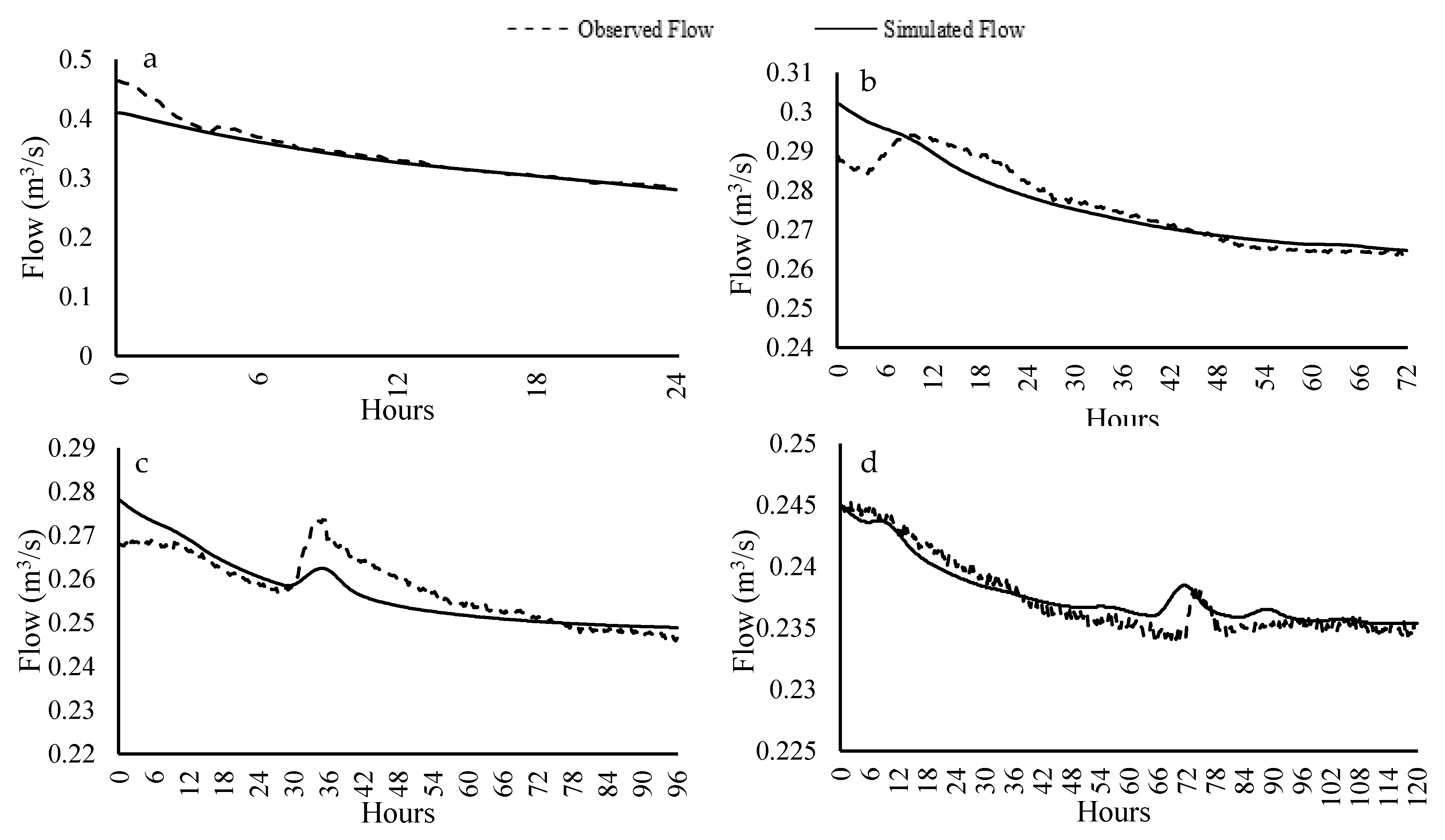
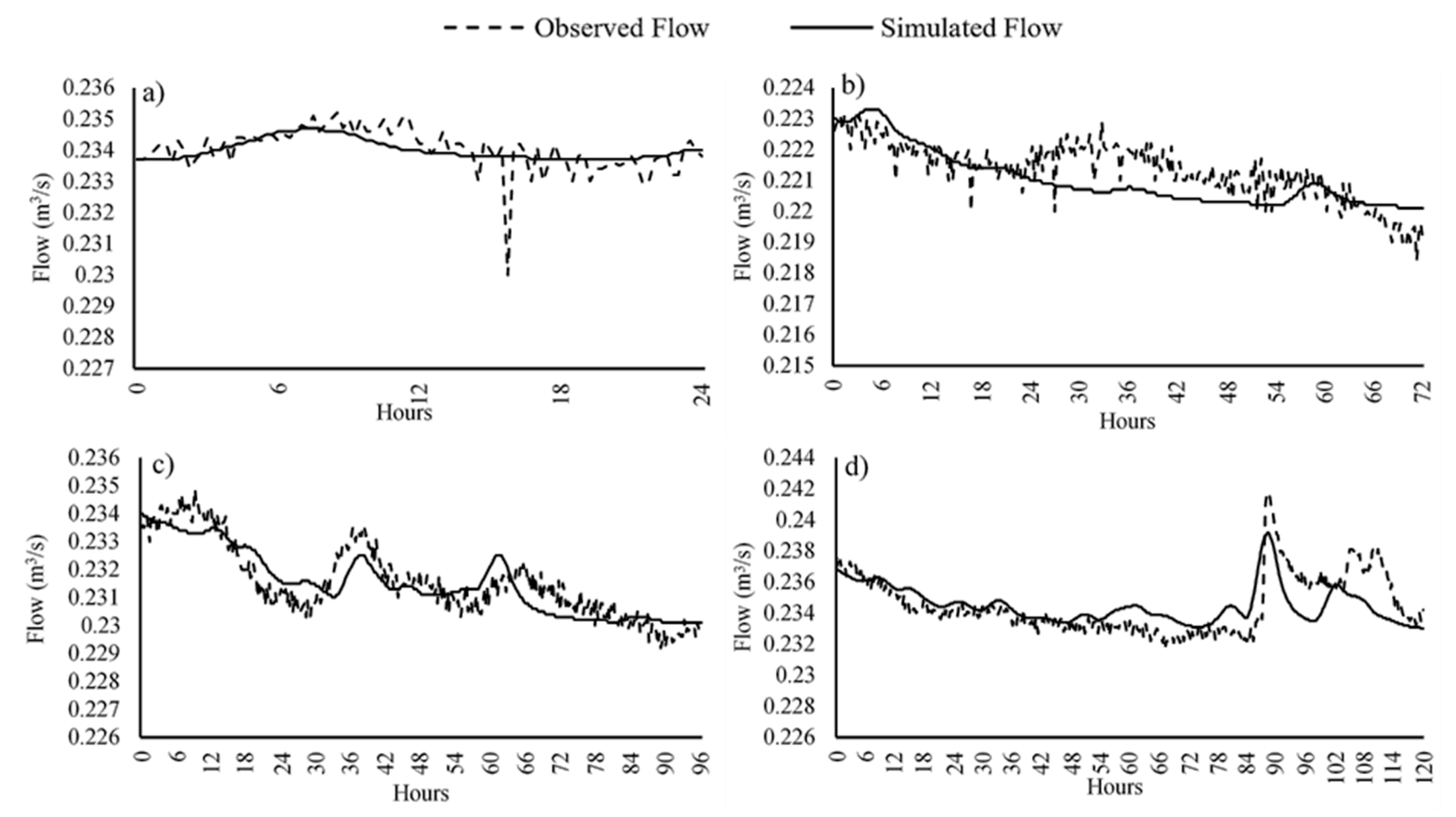
2.3. Model Calibration

Model calibration involved setting the initial baseflow to match that of the observed tributary value for the selected event, then gradually adjusting unobserved model parameters until the modelled output best simulated those of the observed values [35,37,51,52]. Regarding the observed model parameters, infiltration was the key parameter for the hydrological model, it had been collected from October 2019 to August 2021 (with a break from March to July 2020 due to COVID-19), and this parameter could not be changed during the calibration process. The same applied to rainfall and baseflow, as these had been observed through use of the rain gauge and in-channel telemetry. This meant the only adjustable parameters were the lag times and peaking coefficients of the Snyder unit hydrograph transform (Equations (8) and (9)), so these parameters were adjusted through trial-and-error until one set of Snyder values (based on site observations and observed and simulated model output) could be used across all events and produce a similar outcome to the observed flow. This process was undertaken for both the summer and winter models, using available data from the time periods specified in Section 2.2.
The Nash and Sutcliffe (1970) Efficiency (NSE) method was used to determine the closeness-of-fit between the simulated and observed values in calibration. The NSE equation is displayed as follows:
NSE = 1 [ i = 1 n ( Y i o b s Y i s i m ) 2 i = 1 n ( Y i o b s Y m e a n ) 2 ]
where Y i o b s is the observed discharge, Y i s i m is the simulated discharge, and Y m e a n is the mean of observed discharge. Table 2 shows the timeframes of the model calibration for winter and summer models, in addition to the individual and mean NSE values. The NSE method produces a value between 0 and 1, as an indication of how well the simulated dataset ( Y i s i m ) fits the observed dataset ( Y i o b s ) [53,54]. A value of 1 indicates a perfect fit between the two datasets, whereas a value of 0 (or a negative value) indicates a poor fit.
The mean NSE of both the winter and summer calibrations are 0.65. Seen from Table 2, the shorter duration events (24- and 72-h) showed a lower calibration NSE output compared with longer duration events (96- and 120-h). Across the summer calibration events, the lowest NSE value of 0.29 was produced by the 96-h duration, influencing the average NSE. Figure 4 and Figure 5 show the observed and simulated discharge flow graphs for winter and summer model calibration events.

2.4. Model Validation

The model was validated, again, using the NSE method for determination of relationship; however, different storm events were used to those used in calibration (using the same durations) (Table 3) [37,55]. Table 3 shows the timeframes of model validation for winter and summer models, in addition to the individual and mean NSE values.
The mean NSE of the winter validations is 0.87, and summer 0.44. The NSE average for validation events in the winter is high (0.87) indicating that the winter model is very effective at modelling the observed response from the site; whereas the summer validation NSE is 0.44, indicating that the output from the summer models is less accurate than the winter model. Figure 6 and Figure 7 show the observed and simulated discharge flow graphs for winter and summer model validation events.
The chosen calibration and validation datasets were selected primarily due to the scarcity of collected telemetry data from the study site and the timescales from which the data needed to be collected. Therefore, replication of calibration and validation events for the purposes of accuracy was not possible in this instance. Data scarcity for calibration and hydrological modelling is a common occurrence in the field of hydrological modelling. The methods presented throughout this section could be adopted by other researchers in the discipline aiming to simulate similar scenarios to those presented here.

2.5. Model Boundary Conditions

2.5.1. Precipitation and AEP Events

The Flood Estimation Handbook (FEH) was used to generate the design storms used in simulations [56]. Annual exceedance probabilities (AEPs) representing 50% (1 in 2), 10% (1 in 10), 2% (1 in 50), and 1% (1 in 100) rainfall intensities were simulated over 6-, 24-, and 96-h durations [56,57,58]. The 24- and 96-h durations were chosen to test the short-to-medium scale impacts of woodland planting on infiltration. The 6 h duration was chosen due to the requirement of all UK sustainable drainage systems (SuDS) to be tested to this level [59,60]. The rainfall intensities were chosen for similar reasons: the modelled results would enable further understanding regarding the true ability of woodland planting to mitigate runoff from low intensity (50% AEP) to very high intensity (1% AEP) storms, offering insight in to their use as a method of NFM.

2.5.2. Infiltration Data

The collected infiltration data (Section 2.1) were interpreted and included as a primary focus of the modelling process. As this study focuses on the impacts of woodland planting on runoff, the mean infiltration rate (in mL) from every sample site at 10 and 200 cm proximities through both winter and summer (see Section 2.1) were compiled and averaged. The HofE forest planted new woodland every year from 2006 to 2012, but infiltration data were only collected every other year from 2006 (plus a control and the cc.1900 woodland area). To account for the infiltration values of woodland areas planted in the years between the sample plots (2007, 2009, 2011), which needed to be included in the model to fully represent the land cover of the study site, the median value of observed data in both years before and after was calculated. For example, the infiltration value for the unobserved 2007 areas were calculated using the median of the average 2006 and 2008 infiltration data (etc.). Given the lack of observed data and supporting literature in this area, this method is based on mathematical extrapolation and the observation of similar soil texture across the site (Table 1).

2.5.3. Interception

As the sampled woodland is deciduous, interception needed to be considered as it would vary seasonally across the study site [61,62,63]. Interception loss was not empirically monitored for this study; however, it was accounted for, considering the interception loss for grassland to be negligible (<10%) [11,64], and the interception from broadleaves to be between 10–34% (mean 24.25%) [65,66]. FEH values were adjusted in the summer model to account for the rainfall loss due to interception, as simulating the site in both winter and summer with uniform rainfall would not account for any interception loss encountered. This method allows for the inclusion of interception loss in the model without the use of specialised equipment or continuous monitoring, and was an important process, as the influence of interception loss would vary seasonally across the site, both at present and in the future.

2.5.4. Baseflow

Antecedent baseflow had to be calculated, as neglecting to consider this parameter could result in the total discharge from each simulated storm being inaccurate, and not represent true site conditions [67,68]. To calculate the baseflow, telemetry data from both winter and summer periods (Section 2.2) were averaged, the average baseflow for winter models is 0.284 m3 s−1 and for summer models is 0.239 m3 s−1.

2.6. Hydrological Simulations

Three scenarios were simulated using both the winter and summer models with the intention of simulating the peak outflow of the site dependent on varying observed infiltration. Infiltration values for the first simulation scenario were derived from the collected infiltration data from the HofE site (Section 2.1); these data were simulated to reflect the “current HofE (woodland) land cover” as it is at present, and would allow a representation of current site peak discharge. Infiltration values for the second simulation scenarios were altered to represent sites discharge if it was impermeable land cover (developed). The rationale for this originates in Section 1, where it is acknowledged that urbanisation is a key influence of rising flood risk in the UK [1,2]. Infiltration for scenario three were adjusted to represent infiltration collected from the grassland control site (Figure 1). This was to enable a comparison (Section 3) between peak flows from current woodland cover, impermeable land cover, and grassland land cover. It was decided to use the above scenarios as they could be based on collected infiltration data from the site, and provide an accurate representation of the hydrological variations of the sampled study site compared to using published values.

3. Results

Figure 8 shows the peak discharge of the 6-h summer and winter simulations, Table 4 shows the tabulated data with the discrepancy between land cover types shown in comparison to the current HofE site as a percentage.
Figure 8 and Table 4 show that peak runoffs from the impermeable land cover simulations are higher than current and grassland simulations across all modelled storm events in both summer and winter; however, the discrepancy in the winter was slight. Peak flows from HofE land cover were 9.84%, 5.95%, 4.39%, and 3.82% lower than impermeable for a 50%, 10%, 2%, and 1% AEP events, respectively. However, in the summer this difference was higher, with peak flows being 94.55%, 47.62%, 27.91%, and 22.49% greater across 50%, 10%, 2%, and 1% AEP events for impermeable land cover compared to HofE. Grassland peak flows for winter and summer differ significantly, with summer peak flows being 84.71%, 41.67%, 23.52%, and 18.67% higher for 50%, 10%, 2%, and 1% AEP events, respectively. In the winter, grassland shows a 47.54%, 34.52%, 25.44%, and 22.14% reduction in peak flows compared to HofE land cover; this reduction is less in the summer, being 10.91%, 5.71%, 4.07%, and 3.35% for 50%, 10%, 2%, and 1% AEP storms.
Figure 8 and Table 5 show that impermeable cover produces the highest peak flows, compared to the HofE and grassland simulations, over both summer and winter. Current HofE site values are similar to impermeable values throughout the winter; however, this trend is not seen in the summer, where HofE site values are much lower. Grassland produces the lowest peak flows overall; however, grassland values are more similar to current HofE site values in the summer.
Figure 9 shows the peak discharge of the 24-h summer and winter simulations, Table 5 shows the tabulated data with the discrepancy between land cover types shown in comparison to the HofE site as a percentage.
Figure 9 and Table 5 show the highest peak runoff of all simulated land cover types over both winter and summer to be generated by the impermeable land cover; being on average 2.07% higher than HofE land cover in the winter, and 18.31% higher in the summer over all AEPs. The impermeable cover, however, produces the same peak runoff as the HofE site for the 50% AEP in the winter, and peak flows for the impermeable land cover for 10%, 2%, and 1% AEPs in the winter are on average higher than that of the HofE site land cover by only 1.39%. A similar trend is seen in the summer, where peak flows from HofE land cover are only 0.24% lower than impermeable values for all AEPs. All 24-h events show less of a discrepancy between the HofE and impermeable land covers in the winter compared to the 6-h simulations, showing that, as storm duration increases, the flows from impermeable and HofE land cover become more similar in the winter months. Similar to the 6-h duration, grassland peak flows are lower than impermeable and HofE site land cover throughout the winter, however HofE site and grassland peak flows vary less in the summer. In the winter, grassland peak flow is 32.10%, 23.15%, 16.78%, and 14.29% lower than HofE land cover for 50%, 10%, 2%, and 1% AEPs; however, in the summer, grassland is only 4.65%, 2.99%, 2.08%, and 1.79% lower than the current site for all respective AEPs.
Results from the 24-h simulations are similar in trend to those of the 6-h simulations. Impermeable cover produces the highest peak flows over both summer and winter. These values are similar to HofE site discharge in the winter, but not the summer. Grassland produces the lowest peak flows; however, grassland values are more similar to HofE site values in the summer. Summer peak flows for all land cover types are higher than winter values.
Figure 10 shows the peak discharge of the 96-h summer and winter simulations; Table 6 shows the tabulated data with the discrepancy between land cover types shown in comparison to the HofE site as a percentage.
As apparent from Figure 10 and Table 6, the results from the 96-h simulations show similar trends to 6- and 24-h simulations; however, the discrepancy in peak flow between land cover simulations are less notable, as are the seasonal variations in peak flows. Impermeable cover exhibits the highest peak flows compared to HofE and grassland cover; however, this difference is marginal. Impermeable peak flows are 1.25%, 0.99%, 0.80%, and 0.72% higher in the winter, and 5.13%, 2.94%, 1.54%, and 1.39% higher in the summer than HofE land cover for 50%, 10%, 2%, and 1% AEP events, respectively. There is more variation between HofE land cover and grassland in the winter than the summer. Peak flows from the grassland cover are 16.25%, 10.89%, 7.20%, and 6.52% higher than the HofE site in the winter for 50%, 10%, 2%, and 1% AEP events, respectively; however, only showing a difference of 1.28%, 0.98% for 50% and 10% AEP events, and 0 change for the 2%, and 1% AEPs in the summer. Peak flows show less variation between summer and winter for all land cover types, compared to the trends seen in the 6- and 24-h duration simulations.
The results displayed in Figure 10 and Table 6 show that the 96-h duration simulations show less variation in peak flows across all land cover types. There is very little variation in peak flows between land cover types; however, impermeable is slightly higher compared to both current HofE land cover and grassland cover over both summer and winter.
Overall, Figure 8, Figure 9 and Figure 10 and Table 4, Table 5 and Table 6 show that, at present, impermeable cover produces the highest peak flows over all durations and storm intensities compared to other simulated land cover types. However, this is somewhat expected as it is known that the increase in impermeable surface cover is driving the push towards NFM (see Section 1) [1,2,10]. The current land cover of the site shows less of a peak flow compared to impermeable; however, the discrepancy is small and reduces with increased storm duration and intensity. The grassland simulations result in the lowest peak flows, regardless of season or storm scenario. The summer simulations show significantly higher peak flows compared to winter values across all land cover types in the lower duration storms (6- and 24-h); however, this is less significant in the higher duration simulations (96 h).

4. Discussion

The results of the HEC-HMS models presented throughout Section 3 show that woodland planting across the HofE site has reduced peak runoff compared to if the entire site was impermeable, by an average of 6% for 6-h, 2% for 24-h, and 1% for 96-h duration events in the winter; and 48%, 18%, and 2.7% for 6-, 24-, and 96-h durations in the summer. This finding reinforces the benefit that woodland planting can have on increasing the surrounding soils infiltration potential, storage potential, resultantly reducing peak flow from the study area. Whereas the current HofE site does reduced peak flow compared to the impermeable scenario, an entirely grassland catchment shows the greatest reduction in peak flow, being 32%, 21%, and 10% lower than the current site in the winter, and 6%, 2%, and 0.5% lower than the HofE site in the summer for 6-, 24-, and 96-h duration storms, respectively.
It is worth considering that the reduction in peak flows exhibited by grassland compared to both the impermeable and current HofE site reduces as storm duration and intensity increases. This can be explained through considering both the age, and relative root spread of the woodland species sampled [69,70]. As discussed in Section 2.1, aside from the cc.1900 (Quercus Petraea) woodland, the oldest trees sampled were planted in 2006 (Betula Pendula) and the youngest in 2012 (Populus Tremula). Therefore, the 2006 trees have only been developing for 15 years, and the 2012 trees for 9. Betula Pendula reaches its ultimate height at around 60 years from planting, and can live for up to 100 years in total, meaning that the infiltration data collected and simulated in this study is only representative of the beginning of the likely effects that this tree will have, and infiltration will only improve as the tree (and its root system) develop, as the tree approaches maturity [71,72,73,74]. A similar rationale can be applied to the Populus Tremula (2012) tree; the growth of Aspen in the UK slows at around 30 years, and trees can live for 100–120 years [75,76,77]. Thus, if this project was to be replicated in 20 years, tree roots would have developed, breaking up the surrounding soil, and infiltration would likely be greater due to the increased porosity [15,16]. Consequently, the modelled data show that, whilst some reduction in runoff is possible during the growth phase of trees, it will not be until they mature that the total potential reduction is demonstrated in comparison to grassland peak flow reduction.

4.1. Woodland Planting Mentality

The findings of this project are significant when considering the way in which woodland areas are currently managed, regarding the growth and felling of trees and the removal of mature woodlands to make way for either newer areas of woodland or, more significantly, impermeable developments [4,15,78]. It is not uncommon for mature(ing) woodland to be removed to make way for impermeable developments, which significantly alters the local hydrology of an area, sealing-off once permeable areas and excluding them from participating in infiltration processes [4,15,79,80]. Felled trees as a result of development are commonly ‘balanced out’ by planting saplings in alternate locations, however newly planted saplings will not have a comparable moderating impact on flood risk compared with the felled mature trees [18,74,80,81]. This project has demonstrated the above through presenting modelled results, showing that young trees, whilst they do reduce peak flows compared to impermeable land cover, have not yet developed the root systems, and influenced surrounding infiltration rates, to the extent they will with maturity.

4.2. The Influence of Precipitation, Interception, and Model Calibration

Apparent throughout Section 3 is that summer peak flows over all simulated land cover types are higher than the corresponding winter values, this discrepancy reduces in the 96-h duration storm; however, it is more apparent in the 6- and 24-h duration storms. As discussed in Section 2.5.3, the hydrological effects of interception were accounted for in the summer through reducing the precipitation received. Therefore, it would be assumed that summer peak flows would be reduced; however, this is not the case. A reason for this output may be effect of surface pooling (as discussed above); however, another explanation may be due to the parameters used in calibration. The summer and winter models were calibrated individually (Section 2, Table 2), and a set of parameters used for each. The purpose of calibration is to align the observed and simulated outputs as closely as possible over varying events, leaving a final set of values that will produce a reliable output [82,83]. In this case, the only variables that could be adjusted were the components of the Snyder transform method, and the summer model had a quicker lag and a higher peaking coefficient than the winter model. It is possible that this caused the variation seen between summer and winter; however, the calibration was comprehensive, resulting in a final calibration and validation NSE of 0.65 and 0.44 for summer.

4.3. Antecedent Conditions and Results

Grassland continually showing the greatest reduction in peak flow may have been influenced by several external factors. The grassland control site comprises of a sandier soil texture than the pedology of the other sample sites (with the exception of 2010, see Table 1), making it more permeable [84]. This means that when the grassland infiltration data are applied to the whole site to the represent grassland coverage, it is not accounting for variations in soil texture across the site [85,86,87]. Additionally, Table 1 shows that the cc. 1900, 2008, and 2012 sites are comprised of a clay-heavy soil texture, meaning that they are naturally less permeable due to the smaller particle sizes of clay compared with sand [84]. This may be an indication as to why the current HofE site peak flow is higher than that of grassland, particularly in the winter. The winter of 2020 was the fifth wettest on record (329.4 mm/143% higher than the 1981–2010 baseline), and February of 2020 was the wettest ever recorded, with 155 mm of precipitation (258% higher than the 1981–2010 baseline) [88,89]. These dates are within the time periods that winter infiltration data were collected, and the excess rainfall received would have contributed to the study site saturation, influencing infiltration data collection. See Figure 11.
As seen in Figure 11, the variation between antecedent rainfall and clay-saturation throughout winter, and cracking and drying-out throughout summer may have led to infiltration rates being significantly higher than the grassland for the current site simulations in the winter. These effects may also explain the higher peak flows observed throughout summer compared with winter; the increase in surface pooling of the sample sites in the winter (Figure 11a,b) held water in place across the study site. Infiltration would have been slowed due to the clay-geology and antecedent conditions of the site [90,91], meaning runoff was slowed, creating more of a lag between precipitation and peak flow in the winter. Whereas in the summer, the cracking of the ground (Figure 11c,d) reduced infiltration, with the dry clay acting similarly to an impermeable surface. Due to this, rainfall was able to runoff into the watercourse, causing a quicker lag time and a higher peak.

4.4. Study Applications

Whilst antecedent weather conditions and soil texture have influenced the trends seen between woodland and grassland land cover (see Section 3), the clay-heavy soil textures of the sample site are representations of the conditions of many sites around the UK. With the woodland sites being clay, and the ongoing comprehensive infiltration data collection, this project provides an assessment of the impact of NFM (woodland planting) over one of the most impermeable soil types throughout the UK.
Area calculations regarding the coverage of superficial alluvium, clay, peat, and fluvial deposits throughout the UK show that 15% (39,269.24 km2) of UK superficial geology is similar in infiltration to the geology of the HofE site [92]. This demonstrates that the results of this study are significant, and are representative of 15% of UK geology, demonstrating that the results found throughout this study with regard to woodland planting and their runoff reduction capabilities can be extrapolated, furthering the usage of NFM across the UK. This therefore shows that woodland planting can be considered as a method of NFM throughout other areas of the UK, and once could expect to find similar positive results to those found in this study.

5. Conclusions and Future Work

The results from the simulations undertaken in this study have shown that woodland can reduce peak flows when compared to impermeable cover; however, at present, grassland reduces peak flow most in both winter and summer. The values of the data collected throughout is that; if woodland can reduce peak flows at present over a predominantly clay (impermeable) geology, then the value of woodland planting on a site with slightly more permeable geology would show greater results than this study. This presents an opportunity for this research to be extrapolated and applied to other geologies and soil textures, to potentially aid in justifying the use of NFM (woodland planting), as a viable method of increasing infiltration and reducing ruff peaks to watercourses.
Woodland planting is gaining momentum as a method of NFM due to its ability to break up soil and increase infiltration and water storage. This study took infiltration measurements at 10 and 200 cm away from woodland planted at a 2.2 km2 area in Warwickshire, England, from November 2019 until August 2021. Infiltration data were incorporated into two calibrated and validated HEC-HMS models, and the reductions in peak flow for woodland, grassland, and impermeable land cover were quantified. Results of this study show that, across a predominantly clay-site:
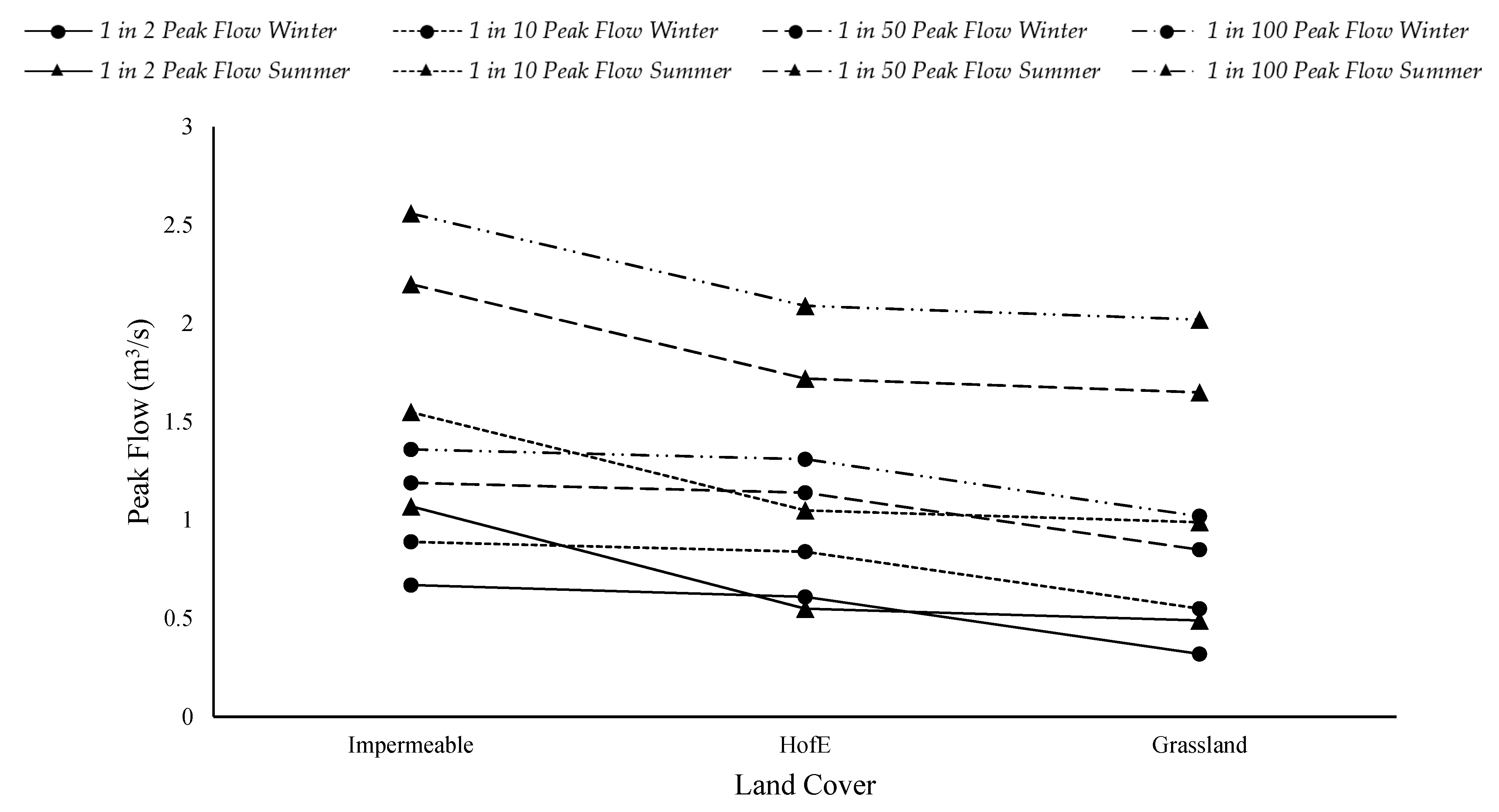
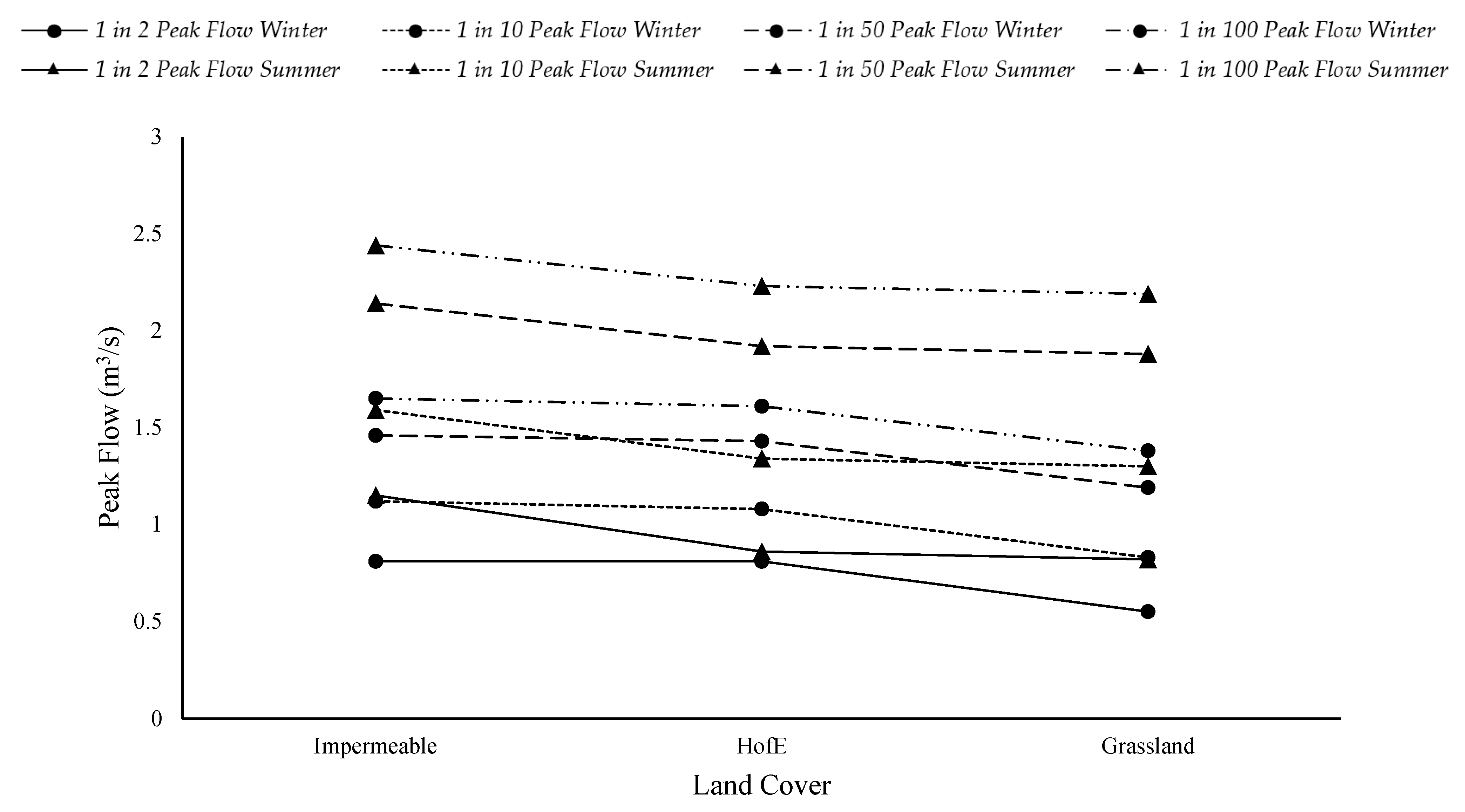
  • Woodland planting across the HofE site shows less of a peak flow compared to impermeable land cover simulations; however, the discrepancy is small and reduces with increase storm duration and intensity.
  • The grassland simulations result in the lowest peak flows, regardless of season or storm scenario.
  • Impermeable land cover produces the highest peak flows throughout all durations and storm intensities compared to woodland and grassland; however, this is somewhat expected as it is known that the increase in impermeable surface cover is aiding the push towards NFM) [1,2,10].
  • The summer simulations show significantly higher peak flows compared to winter values across all land cover types in the lower duration storms (6- and 24-h); however this is less significant in the higher duration simulations (96-h).
The quantified results of this study show woodland to have a positive impact on peak flow reduction after only 15 years (since 2006), and indicate that the impacts will become more significant with root spread as the site matures [16,93]. This study is also representative of a clay-textured site, the same soil texture as 15% of the UK, indicating that if woodland can show a reducing in peak flow across this study site, similar results will be seen in other similar sites. Further to this, the results will likely be more significant in areas inherent of a more permeable soil texture [84].
Additionally, this study has provided insight into how to collect and extrapolate infiltration data and model such information in HEC-HMS. Additionally, it has provided a methodology regarding the calibration and validation of HEC-HMS models where empirical data are sparse. This will enable other authors in the field of hydrology to use this project as a framework when contributing to the knowledge base regarding infiltration, NFM, woodland planting, and hydrology as a whole.
Future work will involve developing a method of projecting the collected infiltration data, with the intention of using the HEC-HMS model to project the ability of woodland planting to mitigate flow and overland runoff into the future, regarding precipitation and baseflow increases in light of climate change.

Author Contributions

Conceptualization, methodology, software, validation, formal analysis, investigation, resources, data curation, writing—original draft preparation N.R.; writing—review and editing, M.R., C.L., M.B.; visualization, N.R., C.L., M.B., M.R.; supervision, C.L., M.B., M.R. All authors have read and agreed to the published version of the manuscript.

Funding

This research received no external funding.

Data Availability Statement

To access the data collected and analysed in this study, please contact the corresponding author: Nathaniel Revell ([email protected]).

Acknowledgments

Special thanks are extended to the HofE forest, in particular Stephen Coffey, for their support and assistance throughout the data collection phase of this project.

Conflicts of Interest

The authors declare no conflict of interest.

References

  1. Ellis, N.; Anderson, K.; Brazier, R. Mainstreaming natural flood management: A proposed research framework derived from a critical evaluation of current knowledge. Prog. Phys. Geogr. Earth Environ. 2021, 1–23. [Google Scholar] [CrossRef]
  2. Ferguson, C.; Fenner, R. The impact of Natural Flood Management on the performance of surface drainage systems: A case study in the Calder Valley. J. Hydrol. 2020, 590, 125354. [Google Scholar] [CrossRef]
  3. Lowe, J.A.; Bernie, D.; Bett, P.; Bricheno, L.; Brown, S.; Calvert, D.; Clark, R.; Edwards, T.; Fosser, G.; Fung, F.; et al. UKCP18 Science Overview Report; Met Office: Exeter, UK, 2019.
  4. Murphy, T.R.; Hanley, M.E.; Ellis, J.S.; Lunt, P.H. Native woodland establishment improves soil hydrological functioning in UK upland pastoral catchments. Land Degrad. Dev. 2021, 32, 1034–1045. [Google Scholar] [CrossRef]
  5. Shuttleworth, E.L.; Evans, M.G.; Pilkington, M.; Spencer, T.; Walker, J.; Milledge, D.; Allott, T.E.H. Restoration of blanket peat moorland delays stormflow from hillslopes and reduces peak discharge. J. Hydrol. X 2019, 2, 100006. [Google Scholar] [CrossRef]
  6. Metcalfe, P.; Beven, K.; Hankin, B.; Lamb, R. A new method, with application, for analysis of the impacts on flood risk of widely distributed enhanced hillslope storage. Hydrol. Earth Syst. Sci. 2018, 22, 2589–2605. [Google Scholar] [CrossRef] [Green Version]
  7. Forbes, H.; Ball, K.; McLay, F. Natural Flood Management Handbook; Scottish Environment Protection Agency: Stirling, UK, 2016; ISBN 978-0-85759-024-4.
  8. Ferguson, C.R.; Fenner, R.A. The potential for natural flood management to maintain free discharge at urban drainage outfalls. J. Flood Risk Manag. 2020, 13, 1–15. [Google Scholar] [CrossRef]
  9. Dadson, S.J.; Hall, J.W.; Murgatroyd, A.; Acreman, M.; Bates, P.; Beven, K.; Heathwaite, L.; Holden, J.; Holman, I.P.; Lane, S.N.; et al. A restatement of the natural science evidence concerning catchment-based “natural” flood management in the UK. Proc. R. Soc. A Math. Phys. Eng. Sci. 2017, 473, 20160706. [Google Scholar] [CrossRef] [PubMed] [Green Version]
  10. Burgess-Gamble, L.; Ngai, R.; Wilkinson, M.; Nisbet, T.; Pontee, N.; Harvey, R.; Kipling, K.; Addy, S.; Rose, S.; Maslen, S.; et al. Working with Natural Processes—Evidence Directory; Environment Agency: Bristol, UK, 2018.
  11. Rachelle, N.; Wilkinson, M.; Nisbet, T.; Harvey, R.; Addy, S.; Burgess-Gamble, L.; Rose, S.; Maslen, S.; Nicholson, A.; Page, T.; et al. Working with Natural Processes—Evidence Directory Appendix 2: Literature Review; Environment Agency: Bristol, UK, 2017.
  12. Wells, J.; Labadz, J.C.; Smith, A.; Islam, M.M. Barriers to the uptake and implementation of natural flood management: A social-ecological analysis. J. Flood Risk Manag. 2020, 13, 1–12. [Google Scholar] [CrossRef]
  13. Lacob, O.; Rowan, J.S.; Brown, I.; Ellis, C. Evaluating wider benefits of natural flood management strategies: An ecosystem-based adaptation perspective. Hydrol. Res. 2014, 45, 774–787. [Google Scholar] [CrossRef] [Green Version]
  14. Dittrich, R.; Ball, T.; Wreford, A.; Moran, D.; Spray, C.J. A cost-benefit analysis of afforestation as a climate change adaptation measure to reduce flood risk. J. Flood Risk Manag. 2019, 12, 1–11. [Google Scholar] [CrossRef] [Green Version]
  15. Chandler, K.R.; Stevens, C.J.; Binley, A.; Keith, A.M. Influence of tree species and forest land use on soil hydraulic conductivity and implications for surface runoff generation. Geoderma 2018, 310, 120–127. [Google Scholar] [CrossRef] [Green Version]
  16. Zhang, D.; Wang, Z.; Guo, Q.; Lian, J.; Chen, L. Increase and Spatial Variation in Soil Infiltration Rates Associated with Fibrous and Tap Tree Roots. Water 2019, 11, 1700. [Google Scholar] [CrossRef] [Green Version]
  17. GOV.UK. £3.9 Million to Drive Innovative Tree Planting. Available online: https://www.gov.uk/government/news/39-million-to-drive-innovative-tree-planting (accessed on 13 July 2021).
  18. Murphy, T. Optimising Oak Woodland Establishment into UK Upland Pastures in the Context of Climate Change; And the Role of Oak Woodland in Soil Hydrological Recovery for Natural Flood Management; University of Plymouth: Plymouth, UK, 2021. [Google Scholar]
  19. Ordnance Survey Ordnance Survey Open Data Download. Available online: https://www.ordnancesurvey.co.uk/opendatadownload/products.html (accessed on 15 February 2019).
  20. Ren, X.; Hong, N.; Li, L.; Kang, J.; Li, J. Effect of infiltration rate changes in urban soils on stormwater runoff process. Geoderma 2020, 363. [Google Scholar] [CrossRef]
  21. Bátková, K.; Miháliková, M.; Matula, S. Hydraulic properties of a cultivated soil in temperate continental climate determined by mini disk infiltrometer. Water 2020, 12, 843. [Google Scholar] [CrossRef] [Green Version]
  22. Rahman, M.A.; Moser, A.; Anderson, M.; Zhang, C.; Rötzer, T.; Pauleit, S. Comparing the infiltration potentials of soils beneath the canopies of two contrasting urban tree species. Urban For. Urban Green. 2019, 38, 22–32. [Google Scholar] [CrossRef]
  23. LaMotte Soil Texture Test Kit. Available online: https://lamotte.com/products/soil/individual-soil-plant-tissue-test-kits/soil-texture-test-1067 (accessed on 15 October 2020).
  24. METER® Group Inc. Mini Disk Infiltrometer User’s Manual; METER: Pullman, WA, USA, 2018. [Google Scholar]
  25. Hepner, H.; Lutter, R.; Tullus, A.; Kanal, A.; Tullus, T.; Tullus, H. Effect of Early Thinning Treatments on Above-Ground Growth, Biomass Production, Leaf Area Index and Leaf Growth Efficiency in a Hybrid Aspen Coppice Stand. Bioenergy Res. 2020, 13, 197–209. [Google Scholar] [CrossRef]
  26. Mauer, O.; Palátová, E. The role of root system in silver birch (Betula pendula Roth) dieback in the air-polluted area of Krušné hory Mts. J. For. Sci. 2003, 49, 191–199. [Google Scholar] [CrossRef] [Green Version]
  27. Perry, T.O. Tree Roots: Facts and Fallacies. J. Arboric. 1982, 8, 197–211. [Google Scholar]
  28. Bagarello, V.; Sgroi, A. Using the single-ring infiltrometer method to detect temporal changes in surface soil field-saturated hydraulic conductivity. Soil Tillage Res. 2004, 76, 13–24. [Google Scholar] [CrossRef]
  29. NextGen. NextGen Spernal, UK. Available online: https://nextgenwater.eu/demonstration-cases/spernal/ (accessed on 16 March 2020).
  30. Terink, W.; Leijnse, H.; van den Eertwegh, G.; Uijlenhoet, R. Spatial resolutions in areal rainfall estimation and their impact on hydrological simulations of a lowland catchment. J. Hydrol. 2018, 563, 319–335. [Google Scholar] [CrossRef]
  31. Roberts, N. Assessing the spatial and temporal variation in the skill of precipitation forecasts from an NWP model. Meteorol. Appl. 2008, 15, 163–169. [Google Scholar] [CrossRef] [Green Version]
  32. Maier, R.; Krebs, G.; Pichler, M.; Muschalla, D.; Gruber, G. Spatial Rainfall Variability in Urban Environments—High-Density Precipitation Measurements on a City-Scale. Water 2020, 12, 1157. [Google Scholar] [CrossRef] [Green Version]
  33. Malik, S.; Pal, S.C. Application of 2D numerical simulation for rating curve development and inundation area mapping: A case study of monsoon dominated Dwarkeswar river. Int. J. River Basin Manag. 2020, 1–11. [Google Scholar] [CrossRef]
  34. Rampinelli, C.G.; Knack, I.; Smith, T. Flood mapping uncertainty from a restoration perspective: A practical case study. Water 2020, 12, 1948. [Google Scholar] [CrossRef]
  35. Derdour, A.; Bouanani, A.; Babahamed, K. Modelling rainfall runoff relations using HEC-HMS in a semi-arid region: Case study in Ain Sefra watershed, Ksour Mountains (SW Algeria). J. Water Land Dev. 2018, 36, 45–55. [Google Scholar] [CrossRef] [Green Version]
  36. Joshi, N.; Bista, A.; Pokhrel, I.; Kalra, A.; Ahmad, S. Rainfall-Runoff Simulation in Cache River Basin, Illinois, Using HEC-HMS. In Proceedings of the World Environmental and Water Resources Congress 2019, Pittsburgh, PA, USA, 19–23 May 2019; American Society of Civil Engineers: Reston, VA, USA, 2019; pp. 348–360. [Google Scholar]
  37. Al-Mukhtar, M.; Al-Yaseen, F. Modeling water quality parameters using data-driven models, a case study Abu-Ziriq marsh in south of Iraq. Hydrology 2019, 6, 24. [Google Scholar] [CrossRef] [Green Version]
  38. Rangari, V.A.; Sridhar, V.; Umamahesh, N.V.; Patel, A.K. Rainfall Runoff Modelling of Urban Area Using HEC-HMS: A Case Study of Hyderabad City. In Advances in Water Resources Engineering and Management; AlKhaddar, R., Singh, R.K., Dutta, S., Kumari, M., Eds.; Lecture Notes in Civil Engineering; Springer: Singapore, 2020; Volume 39, pp. 113–125. ISBN 978-981-13-8180-5. [Google Scholar]
  39. Department for Environment Food & Rural Affairs LIDAR Composite DTM. Available online: https://environment.data.gov.uk/dataset/668881ad-4f8f-42bd-b835-89acf0269496 (accessed on 16 July 2021).
  40. Kafle, M.R. Rainfall-Runoff Modelling of Koshi River Basin Using HEC-HMS. J. Hydogeol. Hydrol. Eng. 2019, 8, 1–9. [Google Scholar]
  41. Ramly, S.; Tahir, W.; Abdullah, J.; Jani, J.; Ramli, S.; Asmat, A. Flood Estimation for SMART Control Operation Using Integrated Radar Rainfall Input with the HEC-HMS Model. Water Resour. Manag. 2020, 34, 3113–3127. [Google Scholar] [CrossRef]
  42. Cunge, J.A. On the subject of a flood propagation computation method (Maskingum method). J. Hydraul. Res. 1969, 7, 205–230. [Google Scholar] [CrossRef]
  43. Dong, X. How to put plant root uptake into a soil water flow model. F1000Research 2016, 5, 1–9. [Google Scholar] [CrossRef] [Green Version]
  44. Broadbridge, P.; Daly, E.; Goard, J. Exact Solutions of the Richards Equation with Nonlinear Plant-Root Extraction. Water Resour. Res. 2017, 53, 9679–9691. [Google Scholar] [CrossRef]
  45. Kuhlmann, A.; Neuweiler, I.; Van Der Zee, S.E.A.T.M.; Helmig, R. Influence of soil structure and root water uptake strategy on unsaturated flow in heterogeneous media. Water Resour. Res. 2012, 48, 1–16. [Google Scholar] [CrossRef]
  46. Blengino Albrieu, J.L.; Reginato, J.C.; Tarzia, D.A. Modeling water uptake by a root system growing in a fixed soil volume. Appl. Math. Model. 2015, 39, 3434–3447. [Google Scholar] [CrossRef]
  47. Difonzo, F.V.; Masciopinto, C.; Vurro, M.; Berardi, M. Shooting the Numerical Solution of Moisture Flow Equation with Root Water Uptake Models: A Python Tool. Water Resour. Manag. 2021, 35, 2553–2567. [Google Scholar] [CrossRef]
  48. Darya, F.; Pavel, K.; Jan, G.; Andrea, J.; Jana, N. The use of Snyder synthetic hydrograph for simulation of overland flow in small ungauged and gauged catchments. Soil Water Res. 2018, 13, 185–192. [Google Scholar] [CrossRef] [Green Version]
  49. Zelelew, D.G.; Melesse, A.M. Applicability of a spatially semi-distributed hydrological model for watershed scale runoff estimation in Northwest Ethiopia. Water 2018, 10, 923. [Google Scholar] [CrossRef] [Green Version]
  50. Koneti, S.; Sunkara, S.L.; Roy, P.S. Hydrological modeling with respect to impact of land-use and land-cover change on the runoff dynamics in Godavari river basin using the HEC-HMS model. ISPRS Int. J. Geo-Inf. 2018, 7, 206. [Google Scholar] [CrossRef] [Green Version]
  51. Met Office UK Climate Averages. Available online: https://www.metoffice.gov.uk/research/climate/maps-and-data/uk-climate-averages/gcq89t680 (accessed on 23 September 2021).
  52. Kumarasamy, K.; Belmont, P. Calibration parameter selection and watershed hydrology model evaluation in time and frequency domains. Water 2018, 10, 710. [Google Scholar] [CrossRef] [Green Version]
  53. Nash, J.E.; Sutcliffe, J.V. River flow forecasting through conceptual models Part I—A discussion of principles. J. Hydrol. 1970, 10, 282–290. [Google Scholar] [CrossRef]
  54. Naik, A.P.; Ghosh, B.; Pekkat, S. Estimating soil hydraulic properties using mini disk infiltrometer. ISH J. Hydraul. Eng. 2019, 25, 62–70. [Google Scholar] [CrossRef]
  55. McMillan, H.K.; Booker, D.J.; Cattoën, C. Validation of a national hydrological model. J. Hydrol. 2016, 541, 800–815. [Google Scholar] [CrossRef]
  56. UK Centre for Ecology and Hydrology. The Flood Estimation Handbook; UK Centre for Ecology and Hydrology: Wallingford, UK, 1999; Available online: https://www.ceh.ac.uk/services/flood-estimation-handbook (accessed on 12 July 2021).
  57. Darwish, M.M.; Tye, M.R.; Prein, A.F.; Fowler, H.J.; Blenkinsop, S.; Dale, M.; Faulkner, D. New hourly extreme precipitation regions and regional annual probability estimates for the UK. Int. J. Climatol. 2021, 41, 582–600. [Google Scholar] [CrossRef]
  58. Wobus, C.; Gutmann, E.; Jones, R.; Rissing, M.; Mizukami, N.; Lorie, M.; Mahoney, H.; Wood, A.; Mills, D.; Martinich, J. Modeled changes in 100 year Flood Risk and Asset Damages within Mapped Floodplains of the Contiguous United States. Nat. Hazards Earth Syst. Sci. Discuss. 2017, 1–21. [Google Scholar] [CrossRef] [Green Version]
  59. Local Authority SuDS Officer Organisation (LASOO). Non-Statutory Technical Standards for Sustainable Drainage; LASOO: London, UK, 2016. [Google Scholar]
  60. Department for Environment, Food and Rural Affairs. Draft National Standards and Specified Criteria for Sustainable Drainage; Defra: London, UK, 2014.
  61. Klamerus-Iwan, A. Different views on tree interception process and its determinants. For. Res. Pap. 2014, 75, 291–300. [Google Scholar] [CrossRef] [Green Version]
  62. Rahman, M.; Ennos, R. What We Know and Don’t Know about the Surface Runoff Reduction Potential of Urban Trees; Technical Report; Technical University of Munich: Munich, Germany, 2016; pp. 1–14. [Google Scholar]
  63. Komatsu, H.; Kume, T.; Otsuki, K. Increasing annual runoff-broadleaf or coniferous forests? Hydrol. Process. 2011, 25, 302–318. [Google Scholar] [CrossRef]
  64. Nisbet, T. Water Use by Trees; Information Note FCIN065; Forestry Commission: Edinburgh, UK, 2005; pp. 1–8.
  65. Calder, I.R. Assessing the water use of short vegetation and forests: Development of the Hydrological Land Use Change (HYLUC) model. Water Resour. Res. 2003, 39, 1–8. [Google Scholar] [CrossRef]
  66. Lunka, P.; Patil, S.D. Impact of tree planting configuration and grazing restriction on canopy interception and soil hydrological properties: Implications for flood mitigation in silvopastoral systems. Hydrol. Process. 2016, 30, 945–958. [Google Scholar] [CrossRef] [Green Version]
  67. Schütte, S.; Schulze, R.E. Projected impacts of urbanisation on hydrological resource flows: A case study within the uMngeni Catchment, South Africa. J. Environ. Manag. 2017, 196, 527–543. [Google Scholar] [CrossRef]
  68. Yusop, Z.; Chan, C.H.; Katimon, A. Runoff characteristics and application of HEC-HMS for modelling stormflow hydrograph in an oil palm catchment. Water Sci. Technol. 2007, 56, 41–48. [Google Scholar] [CrossRef] [Green Version]
  69. Randrup, T.B. A review of tree root conflicts with sidewalks, curbs, and roads. Urban Ecosyst. 2001, 5, 209–225. [Google Scholar] [CrossRef]
  70. Birkinshaw, S.J.; Bathurst, J.C.; Robinson, M. 45 years of non-stationary hydrology over a forest plantation growth cycle, Coalburn catchment, Northern England. J. Hydrol. 2014, 519, 559–573. [Google Scholar] [CrossRef] [Green Version]
  71. Lee, S.J.; Connolly, T.; Wilson, S.M.; Malcolm, D.C.; Fonweban, J.; Worrell, R.; Hubert, J.; Sykes, R.J. Early height growth of silver birch (Betula pendula Roth) provenances and implications for choice of planting stock in Britain. Forestry 2015, 88, 484–499. [Google Scholar] [CrossRef] [Green Version]
  72. Kuparinen, A.; Savolainen, O.; Schurr, F.M. Increased mortality can promote evolutionary adaptation of forest trees to climate change. For. Ecol. Manag. 2010, 259, 1003–1008. [Google Scholar] [CrossRef]
  73. Zeltiņš, P.; Gailis, A.; Jansons, J.; Katrevičs, J.; Jansons, Ā. Genetic Parameters of Growth Traits and Stem Quality of Silver Birch in a Low-Density Clonal Plantation. Forests 2018, 9, 52. [Google Scholar] [CrossRef] [Green Version]
  74. Hynynen, J.; Niemisto, P.; Vihera-Aarnio, A.; Brunner, A.; Hein, S.; Velling, P. Silviculture of birch (Betula pendula Roth and Betula pubescens Ehrh.) in northern Europe. Forestry 2010, 83, 103–119. [Google Scholar] [CrossRef]
  75. CAB International. The CABI Encyclopedia of Forest Trees; CABI Publishing: Wallingford, UK, 2013; ISBN 9781780642369. [Google Scholar]
  76. Savill, P. The Silviculture of Trees Used in British Forestry, 3rd ed.; CABI Publishing: Wallingford, UK, 2019. [Google Scholar]
  77. MacKenzie, N.A. Ecology, Conservation and Management of Aspen: A Literature Review; CABI Publishing: Wallingford, UK, 2010. [Google Scholar]
  78. Thomas, H.; Nisbet, T.R. Slowing the Flow in Pickering: Quantifying the Effect of Catchment Woodland Planting on Flooding Using the Soil Conservation Service Curve Number Method. Int. J. Saf. Secur. Eng. 2016, 6, 2–20. [Google Scholar]
  79. Hankin, B.; Chappell, N.; Page, T.; Kipling, K.; Whitling, M.; Burgess-Gamble, L. Mapping the Potential for Working with Natural Processes—Technical Report; Environment Agency: Bristol, UK, 2018.
  80. Cooper, M.M.D.; Patil, S.D.; Nisbet, T.R.; Thomas, H.; Smith, A.R.; McDonald, M.A. Role of forested land for natural flood management in the UK: A review. Wiley Interdiscip. Rev. Water 2021, 8, 1–16. [Google Scholar] [CrossRef]
  81. Archer, N.A.L.; Bonell, M.; Coles, N.; MacDonald, A.M.; Auton, C.A.; Stevenson, R. Soil characteristics and landcover relationships on soil hydraulic conductivity at a hillslope scale: A view towards local flood management. J. Hydrol. 2013, 497, 208–222. [Google Scholar] [CrossRef] [Green Version]
  82. Sharu, E.H. Development of HEC-HMS Model for Flow Simulation at Dungun River Basin Malaysia. Adv. Agric. Food Res. J. 2020, 1, 1–16. [Google Scholar] [CrossRef]
  83. Hamdan, A.N.A.; Almuktar, S.; Scholz, M. Rainfall-Runoff Modeling Using the HEC-HMS Model for the Al-Adhaim River Catchment, Northern Iraq. Hydrology 2021, 8, 58. [Google Scholar] [CrossRef]
  84. Folorunso, O.; Aribisala, J. Effect of Soil Texture on Soil Infiltration Rate. Arch. Curr. Res. Int. 2018, 14, 1–8. [Google Scholar] [CrossRef]
  85. Silber, A. Chemical Characteristics of Soilless Media. In Soilless Culture; Elsevier: Amsterdam, The Netherlands, 2019; pp. 113–148. ISBN 9780444636966. [Google Scholar]
  86. Rabot, E.; Wiesmeier, M.; Schlüter, S.; Vogel, H.J. Soil structure as an indicator of soil functions: A review. Geoderma 2018, 314, 122–137. [Google Scholar] [CrossRef]
  87. Sun, D.; Yang, H.; Guan, D.; Yang, M.; Wu, J.; Yuan, F.; Jin, C.; Wang, A.; Zhang, Y. The effects of land use change on soil infiltration capacity in China: A meta-analysis. Sci. Total Environ. 2018, 626, 1394–1401. [Google Scholar] [CrossRef]
  88. The Met Office Record Breaking Rainfall. Available online: https://www.metoffice.gov.uk/about-us/press-office/news/weather-and-climate/2020/2020-winter-february-stats (accessed on 11 June 2021).
  89. Davies, P.A.; McCarthy, M.; Christidis, N.; Dunstone, N.; Fereday, D.; Kendon, M.; Knight, J.R.; Scaife, A.A.; Sexton, D. The wet and stormy UK winter of 2019/2020. Weather 2021, wea.3955. [Google Scholar] [CrossRef]
  90. Groenendyk, D.G.; Ferré, T.P.A.; Thorp, K.R.; Rice, A.K. Hydrologic-process-based soil texture classifications for improved visualization of landscape function. PLoS ONE 2015, 10, e0131299. [Google Scholar] [CrossRef] [Green Version]
  91. Leung, A.K.; Boldrin, D.; Liang, T.; Wu, Z.Y.; Kamchoom, V.; Bengough, A.G. Plant age effects on soil infiltration rate during early plant establishment. Geotechnique 2018, 68, 646–652. [Google Scholar] [CrossRef] [Green Version]
  92. British Geological Survey 1:625k Bedrock and Superficial UK Geology. Available online: https://www.bgs.ac.uk/datasets/bgs-geology-625k-digmapgb/ (accessed on 15 June 2021).
  93. Xie, C.; Cai, S.; Yu, B.; Yan, L.; Liang, A.; Che, S. The effects of tree root density on water infiltration in urban soil based on a Ground Penetrating Radar in Shanghai, China. Urban For. Urban Green. 2020, 50, 126648. [Google Scholar] [CrossRef]
Figure 1. Sample sites, sampling locations, rain gauge, and telemetry locations [19]. Data is reproduced under the open government license.
Water 13 03039 g001
Figure 2. (a) MDI performing measurement at the study site; (b) 10 and 200 cm proximity MDI sample replication points outlined in orange.
Water 13 03039 g002
Figure 3. HEC-HMS hydrological model. Brown indicates forested plots, green indicates grassland only plots, grey indicates impermeable surfaces, and cross-hatching represents infiltration sample plots.
Water 13 03039 g003
Figure 4. Observed and simulated discharge for winter model calibration events; (a) is the 24-h duration, (b) is the 72-h duration, (c) is the 96-h duration and (d) is the 120-h duration.
Water 13 03039 g004
Figure 5. Observed and simulated discharge for summer model calibration events; (a) is the 24-h duration, (b) is the 72-h duration, (c) is the 96-h duration and (d) is the 120-h duration.
Water 13 03039 g005
Figure 6. Observed and simulated discharge for winter model validation events; (a) is the 24-h duration, (b) is the 72-h duration, (c) is the 96-h duration and (d) is the 120-h duration.
Water 13 03039 g006
Figure 7. Observed and simulated discharge for summer model validation events; (a) is the 24-h duration, (b) is the 72-h duration, (c) is the 96-h duration and (d) is the 120-h duration.
Water 13 03039 g007
Figure 8. Output peak flows from all simulated land cover types.
Water 13 03039 g008
Figure 9. Output peak flows from all simulated land cover types (24-h).
Water 13 03039 g009
Figure 10. Output peak flows from all simulated land cover types (96-h).
Water 13 03039 g010
Figure 11. (a,b) saturation of the 2006 sample site during winter data collection, (c) cracking of the 2006, and (d) 2008 sample sites in the winter (locations can be identified using Figure 1).
Water 13 03039 g011
Table 1. Soil percentiles and texture classification of each sample site.
Sample SiteSand %Silt %Clay %UK Soil Classification
Control532027SaCLSandy clay loam
Pre-1900474013SSLSandy silt loam
2006202060CClay
2008132067CClay
2010533314SaLSandy loam
2012331354CClay
Table 2. Calibration events for winter and summer models. Note that the start and end time describes the time at which modelling began, not the start of the storm event.
Calibration Events
Winter
Duration (h)Start DateStart TimeEnd DateEnd TimeRainfall (mm)NSE
2416 January 202104:0017 January 202104:001.80.41
7217 January 202116:0020 January 202116:0010.600.30
9630 November 201904:0004 December 201904:000.800.92
12008 October 202007:0013 October 202007:006.700.98
Summer
2409 September 202003:0010 September 202003:001.200.62
7219 August 202007:0022 August 202007:0019.600.80
9601 August 202001:0005 August 202001:007.900.29
12028 August 202007:0002 September 202007:0013.400.89
Table 3. Validation events for winter and summer models. Note that the start and end time describes the time at which modelling began, not the start of the storm event.
Validation Events
Winter
Duration (h)Start DateStart TimeEnd DateEnd TimeRainfall (mm)NSE
2414 January 202104:3015 January 202104:301.100.90
7206 December 202007:0009 December 202007:002.700.81
9602 November 202001:0006 November 202001:006.700.87
12013 October 202007:0018 October 202007:004.500.88
Summer
2404 September 202002:0005 September 202002:000.700.35
7209 September 202022:0012 September 202022:001.000.23
9604 September 202022:0008 September 202022:004.200.74
12030 August 202002:0004 September 202002:008.000.42
Table 4. Peak discharge of all simulated land cover types over a 6-h duration rainfall event.
6-hAEP %HofE (Wooded Land Cover)
(m3 s−1)
Impermeable Land Cover
(m3 s−1)
Change from HofE (as %)Grassland Land Cover
(m3 s−1)
Change from HofE (as %)
Winter
Peak volume 500.610.679.840.32−47.54
100.840.895.950.55−34.52
21.141.194.390.85−25.44
11.311.363.821.02−22.14
Summer
Peak volume 500.551.0794.550.49−10.91
101.051.5547.620.99−5.71
21.722.227.911.65−4.07
12.092.5622.492.02−3.35
Table 5. Peak discharge of all simulated land cover types over a 24-h duration rainfall event.
24-hAEP %HofE (Wooded Land Cover)
(m3 s−1)
Impermeable Land Cover
(m3 s−1)
Change from HofE (as %)Grassland Land Cover
(m3 s−1)
Change from HofE (as %)
Winter
Peak volume 500.610.679.840.32−47.54
100.840.895.950.55−34.52
21.141.194.390.85−25.44
11.311.363.821.02−22.14
Summer
Peak volume 500.551.0794.550.49−10.91
101.051.5547.620.99−5.71
21.722.227.911.65−4.07
12.092.5622.492.02−3.35
Table 6. Peak discharge of all simulated land cover types over a 96-h duration rainfall event.
96-hAEP %HofE (Wooded land Cover)
(m3 s−1)
Impermeable Land Cover
(m3 s−1)
Change from HofE (as %)Grassland Land Cover
(m3 s−1)
Change from HofE (as %)
Winter
Peak volume 500.610.679.840.32−47.54
100.840.895.950.55−34.52
21.141.194.390.85−25.44
11.311.363.821.02−22.14
Summer
Peak volume 500.551.0794.550.49−10.91
101.051.5547.620.99−5.71
21.722.227.911.65−4.07
12.092.5622.492.02−3.35
Publisher’s Note: MDPI stays neutral with regard to jurisdictional claims in published maps and institutional affiliations.

