Seasonal Variations of the Depletion Factor during Recession Periods in the Senegal, Gambia and Niger Watersheds

1
G-EAU, IRD (AgroParisTech, Cirad, IRSTEA, MontpellierSupAgro, Univ Montpellier), BP5095, 34196 Montpellier, France
2
Département de Géographie, FLSH-UCAD, BP 5005 Dakar-Fann, Senegal
*
Author to whom correspondence should be addressed.
Water 2020, 12(9), 2520; https://doi.org/10.3390/w12092520
Submission received: 17 July 2020
/
Revised: 27 August 2020
/
Accepted: 29 August 2020
/
Published: 9 September 2020
(This article belongs to the Special Issue Multiscale Impacts of Anthropogenic and Climate Changes on Tropical and Mediterranean Hydrology)
Abstract
:The daily depletion factor K describes the discharge decrease of rivers only fed by groundwater in the absence of rainfall. In the Senegal, Gambia and Niger river basins in West Africa, the flow recession can exceed 6 months and the precise knowledge of K thus allows discharge forecasts to be made over several months, and is hence potentially interesting for hydraulic structure managers. Seasonal flow recession observed at 54 gauging stations in these basins from 1950 to 2016 is represented by empirical and usual conceptual models that express K. Compared to conventional conceptual models, an empirical model representing K as a polynomial of the decimal logarithm of discharge Q gives better representations of K and better discharge forecasting at horizons from 1 to 120 days for most stations. The relationship between specific discharge Qs and K, not monotonous, is highly homogeneous in some sub-basins but differs significantly between the Senegal and Gambia basins on the one hand and the Niger basin on the other. The relationship K(Q) evolves slightly between three successive periods, with values of K generally lower (meaning faster discharge decrease) in the intermediate period centered on the years 1970–1980. These climate-related interannual variations are much smaller than the seasonal variations of K.
1. Introduction
1.1. Background, Context
According to [1], “the decrease of discharge corresponding to the emptying of groundwater without any precipitation is called the flow recession of a river”. This stream flow regime has been the subject of numerous studies, including reviews [2,3].
According to these authors, the flow recession concerns “all natural storages feeding the stream, including unsaturated grounds and lakes”. Among the oldest works, [4] established the differential equation governing the discharge of an aquifer in a homogeneous ground. This author derives two conceptual models that give the discharge rate of the groundwater into a river under certain boundary conditions. The first, which is the most widely used recession model [1,5], is described as linear [2]. Assuming a thick aquifer whose free surface is close to the horizontal, it expresses the discharge Q at time T as a function of discharge Q0 at time T0, with a constant α characteristic of the ground and the dimensions of the aquifer and dependent on the unit of time (but independent of T0), or with a constant K equal to e−α, called “depletion factor” [6]:
The second model proposed by [4], described as non-linear [2], assumes a groundwater table limited by an impermeable horizontal bottom and vertical wall, draining into the watercourse at its base. It is expressed in this way, with a constant σ0 characteristic of the soil and the dimensions of the aquifer and depending on both the unit of time T and the initial time T0:
According to [5], the relationship (1) first applied by [7] is generally referred to as the “Maillet formula”, while the relationship (2), used by [8] for African rivers, is generally referred to as the “Tison formula”.
Reference [9] shows that these two formulas are particular cases of a more general conceptual model (Q = ZVm) that represents the emptying of a reservoir under the assumption of a discharge Q proportional to a certain m power of the remaining water volume V, with a proportionality constant Z. This author finds the Maillet equation (1) with m equal to 1, his model then representing the emptying of a vertical cylinder by a porous plug at its base [1]. When m is different from 1, he obtains the following result where V0 is the volume remaining at time T0:
with m = 2, the “Coutagne equation” (3) gives the Tison equation (2) and represents the emptying of a vertical cylindrical reservoir by a parabolic spillway with a vertical axis [10].
Some authors propose the empirical addition of a constant term W to Maillet’s equation [11,12,13,14,15], to Tison’s equation (Maillet, in [4]) or to that of Coutagne [9,16]. The relationships thus obtained are called here “generalized Maillet equation” (6) and “generalized Coutagne equation” (7):
in these relationships, the parameters α and σ0 depend on the time unit and σ0 also depends on the initial time T0, which can be set arbitrarily. With the relationship (6), the recession can be represented indifferently from the flow rates QA and QB at the initial times TA and TB if the relationship (8) is respected. With the relationship (7), QA and QB at the initial times TA and TB, associated with σA and σB, must verify the relationship (9).
Relationship (10) is a particular case of the generalized Coutagne equation obtained after changing the variable by translation over time. It is used in different forms with the parameters λ, μ and r by some authors [13,17,18,19,20,21]:
Reference [22] proposes an empirical adaptation of the Maillet formula, by a change of variable with a power function over time. So the “Horton formula”, sometimes referred to as the double exponential [2], is expressed as follows with the parameters β and p:
Finally, recession is often represented by the sum of Maillet formulas [4,6,23,24,25,26] or Maillet formulas and Tison formulas [27].
The most commonly used conceptual models to represent recession, listed by [3,28], can all be represented by the generalized Maillet (6), generalized Coutagne (7) or Horton (11) formulas, or by combinations of these formulas. The calibration of these conceptual or empirical models is usually based on the analysis of certain relationships in observed data, using either a graphical or least squares method. These relationships, sometimes interpreted as envelope curves to distinguish the origin of the flows (slow variable feeding by the aquifers and more rapid variable feeding for the other origins), are as follows:
- Relationship between Q(T) and Q(T + dT): correlation method. With dT = 1 day, [29] uses this mean relationship as an empirical recession curve, and [30] represents the upper envelope curve by a line passing through the origin, whose slope corresponds to the depletion factor K of the Maillet equation (1). With dT = 5 days, [31] represents the mean relationship by a line passing through the origin, whose slope corresponds to K5.
- Relationships between T and Log(Q) established for different recession sequences. Reference [32] uses these relationships and interprets their slope in each point as −α (Maillet’s formula). He derives an empirical model giving α as a function of Q and T. Ref. [33] set the Maillet formula by representing the relationships obtained for the different sequences by linear relationships, whose common slope corresponds to −α.
- Relationship between Log(Q) and Log(−dQ/dT). Refs. [34,35] represent the low envelope curve of this relationship by sections of linear functions, whose slope and ordinate at the origin correspond respectively to (n + 1)/n and Log(nσ0Q0−1/n), where n and σ0 are the parameters of the Coutagne equation (3). The 3/2 slope obtained for low flows gives n = 2, according to the Tison equation (2). Reference [36] obtains an average relationship with a slope close to 1, according to the Maillet equation (1).
- Relationship between Q and −dQ/dT. For different periods varying in distance from the beginning of recession, [37] represent the upper and lower envelopes of this relationship by lines passing through the origin, whose slope corresponds to the α parameter of the Maillet equation (1). These authors find that α is not very variable for low envelopes associated with baseflow from groundwater, while it decreases over time for high envelopes.
Each of the above methods, therefore, consists in representing, generally by one or more lines, a relationship between a primary variable (Q(T), T, Log(Q) or Q) and a secondary variable (Q(T + dT), Log(Q), Log(−dQ/dT) or −dQ/dT). This can be problematic for rivers in West Africa, where Q and −dQ/dT can decrease by several orders of magnitude during recession sequences spread over several months. Any elementary function adjusted to Q or −dQ/dT by the least squares method can then lead to very large relative errors for the lowest values of Q(T + dT) or −dQ/dT. Conversely, adjusting a function on logarithms of Q or −dQ/dT can be unfavorable and allow large relative errors for the highest values of Q or −dQ/dT.
The method used by [5,38], derived from the correlation method, does not have these disadvantages. From the mean Qm of observed discharge, these authors calibrate the Maillet equation by calculating the ratio Qm(T + dT)/Qm(T), interpreted as KdT. They deduce K from the resulting ratios calculated for different dT values.
To study the flow recession on the Senegal River basin in West Africa, reference [39] uses a quite similar method to the previous one. Instead of Qm(T + dT)/Qm(T), they calculate for dT = 1 day the daily values of Q(T + dT)/Q(T) that corresponds to the daily depletion factor K of the Maillet formula. Despite their wide dispersion between 0.5 and 1, the values obtained show an average seasonal evolution that can be represented by an empirical function of time T, which is counted from an origin set at the same date each year. This function represents K with the same accuracy for very different discharges, which is an advantage over the methods mentioned above. For most of the stations analyzed, K does not vary monotonously with T: from a low value at the beginning of recession, K increases to a maximum value and then decreases rapidly until the end of recession. Among the commonly used conceptual models, only the generalized Coutagne model (7), used with a negative W, makes it possible to represent such a variation of K (for a demonstration see text S1).
1.2. Objectives of the Project
This study, which is an extension of the work of [39], focuses on the depletion factor K in the Senegal, Gambia and Niger river basins in West Africa. Precise knowledge of K, always situated between 0 and 1 by definition, is of interest for two main reasons:
- The knowledge of groundwater, since K describes the recharge of the river flow by the groundwater in the absence of rainfall. A high K coefficient, close to 1, corresponds to a slow decrease in the discharge, thanks to important contributions from the water tables. Conversely, a low K coefficient corresponds to a rapid decrease in the flow of rivers, with little discharge supply from groundwater. K thus characterizes the capacity of groundwater to supply rivers. This capacity depends both on geological and pedological characteristics (transmissivity, storage, permeability) and on the abundance of previous rainfall inputs to the basin.
- The forecasting of discharge during recession periods, which can extend more than 6 months in the region. Flow forecasts can, therefore, be made over very long horizons of several months, which can be of great interest to managers of hydraulic structures such as dams.
For 54 stations located in the Senegal, Gambia and Niger river basins, we model the flow recession of rivers from observed values of the daily depletion factor K over the period 1950–2016. In addition to the most frequently used Maillet model (K constant), other models are tested to describe seasonal variations of K as a function of time T or discharge Q, using formulas whose form is empirical or imposed by the generalized Coutagne equation (7). We compare the performance of the different models in representing K and in forecasting discharge Q at all possible forecast horizons during the recession sequences enabled by the models. Finally, we compare seasonal variations and interannual variations of K.
The following sections present the method, data, results and conclusions of the study. All dates are expressed in day/month/year.
2. Materials and Methods
2.1. Methods
2.1.1. Observed Values of the Daily Depletion Factor K
According to equation (1), the daily depletion factor K(T) is equal to Q(T + 1)/Q(T) with T expressed in days. But to limit their dispersion, its values are calculated over 3 consecutive days from the flows observed at times T − 1 and T + 2:
Only the values K(T) based on flows Q(T − 1) and Q(T + 2) belonging to the same recession sequence are retained, with T verifying the following 3 conditions:
- C1: times T − 2 to T + 2 fall within the usual recession period, which starts and ends on invariable dates T1 and T2, expressed in days/months;
- C2: between times T − 2 and T + 2, the discharge is known at a daily time step with no missing data and decreases in the broad sense, meaning that Q(T + k) ≤ Q(T + k − 1) for all integer numbers k between −1 and 2;
- C3: the discharge Q(T + 2) is greater than a minimum threshold Qthr arbitrarily set at 0.1 m3·s−1.
2.1.2. Analyses Performed
We tested 5 models to represent the depletion factor K:
- The Maillet’s conceptual model (model 0). This model was chosen because it is the most often used model of recession.
- An empirical model representing K as a function of time (model 1).
- An empirical model representing K as a function of discharge (model 2).
- The generalized Coutagne conceptual model. This model was chosen because it is the only usual conceptual model capable of representing the non-monotonic evolution of K observed in the Senegal River basin during the recession period (see above). The generalized Coutagne model is used to represent K as a function of time (model 3) or as a function of discharge (model 4).
For each station, we represent the seasonal variations of K(T) with these five models calibrated using the least squares method:
- model 0: average Km of the observed values of K(T), constant value compatible with the Maillet formula;
- model 1: empirical polynomial function f of the delay D(T) elapsed between the initial time T0 (invariable, expressed in day/month) and T, defined with parameters A1 to A6 by:
- model 2: empirical function g of the discharge Q(T), polynomial of the decimal logarithm of Q defined with parameters B1 to B6 by:
- model 3: function fb of the delay D(T), verifying with the parameters Q0, W, σ0 and n the relationship (15) imposed by the generalized Coutagne formula:
- model 4: function gb of the discharge Q(T), verifying with the parameters Q0, W, σ0 and n the relationship (16) imposed by the generalized Coutagne formula:
Calibrated on all the N observed values of K, each of these models makes it possible to represent hydrographs Q(T) that differ between different recession periods by homothety for models 0, 1 and 3 and by time translation for models 0, 2 and 4 (for a demonstration see Text S2). The models are classified according to the Nash and Sutcliffe efficiency coefficient CNSE0 relative to the N modeled K values (CNSE0 = 0 for model 0 based on the Maillet formula), with Ra rank ranging from 1 for maximum CNSE0 to 5 for minimum CNSE0. The models’ ability to forecast recession flows is then evaluated for all entire H forecast horizons between 1 and 120 days.
Let a sequence of uninterrupted recession be limited by the times Tb − 2 and Tb + Np + 1, during which conditions C1 to C3 are checked for any T between Tb and Tb + Np − 1. These conditions make it possible to calculate Np observed values of K with equation (12) between the times Tb and Tb + N − 1, and also to calculate Np × (Np + 1)/2 forecasted discharges over the sequence with each recession model: Np values are forecast on a first sub sequence at times Tb + 1 to Tb + Np from the discharge observed at time Tb, for horizons H from 1 to Np days; Np − 1 values are forecast on a second sub sequence at times Tb + 2 to Tb + Np from the discharge observed at time Tb + 1, for horizons H from 1 to Np − 1 days; a value is predicted on a Npth sub sequence at time Tb + Np from the discharge observed at time Tb + Np − 1, for a horizon of 1 day. For each sub sequence, each forecast discharge is calculated with the recession model applied to the previous day’s discharge (observed for the first of the sub sequence and forecast for the following ones).
The accuracy of the forecast discharges is evaluated as follows: for each horizon H, using the relative standard error Rrmse (ratio between the standard error Se and the average Qm of the corresponding observed flows) and the Nash and Sutcliffe efficiency coefficient CNSE1 for the Ne values forecast at horizon H over all the recession periods defined above; using the CNSE2 for the Nt values predicted at the different horizons (with ).
2.2. Data
The data used are the average daily discharges observed under natural conditions between 1950 and 2016 at 54 gauging stations (Table 1, Table 2 and Table 3 and Figure 1) located in the upper basins of the Senegal River (up to Kaédi), the Gambia River (in Senegal, upstream of Gouloumbo) and the Niger River (in Mali, up to Ansongo). These data come from the former ORSTOM/IRD databases developed and enriched through various projects [39,40,41,42,43], often carried out in partnership with data-producing or -managing organizations (Direction Nationale de l’Hydraulique du Mali, Organisation pour la Mise en Valeur du fleuve Gambie, Organisation pour la Mise en Valeur du fleuve Sénégal, Service de Gestion et de Planification des Ressources en Eau du Sénégal).
Among the discharges obtained by translating the levels observed at the stations, all the reconstructed values are excluded from the analyses of the recession regime. Data influenced by large reservoir dams upstream (at Soukoutali and downstream from 1987 on the Senegal basin (Manantali dam); at Sélingué and downstream from 1981 on the Niger basin (Sélingué dam)) are also excluded.
The stations analyzed control basins whose area ranges from 18 to more than 280,000 km2. Their mean interannual specific discharges Qsm (calculated by integrating certain reconstituted values) vary between 0.56 and 17.59 l·s−1·km−2 (Table 1, Table 2 and Table 3). The study, therefore, concerns very diverse stations, for which the data also cover the study period in a very variable way (varying numbers of missing observations).
The annual peak flood in the region occurs generally in mid September, except in the Inner Niger Delta (DIN) and downstream, where the flood mainly formed upstream spreads very slowly (Figure 2). The general decrease in flow occurs then and persists until the arrival of flows caused by the following monsoon, usually in May or June or even in July downstream of the DIN. The origin T0 of the times is therefore set to the previous 15 September for all stations and the T1 and T2 start and end dates of the usual recession period are set to 15 September and 31 May, respectively, except for the following stations:
- T1 = 15 October and T2 = 30 June for Akka on Niger (rank 50), due to the slower spread of flows as they pass the DIN;
- T1 = 15 November and T2 = 31 July for for Diré, Koryoumé, Tossaye and Ansongo on Niger (ranks 51 to 54), for the same reasons as Akka;
- T1 = 15 September and T2 = 30 April for Moussala and Siramakana in the Senegal watershed (ranks 12 and 17), Diaguery and Niokolokoba in the Gambia watershed (ranks 29 and 30) and Manankoro in the Niger watershed (rank 42), where the discharge ceases each year before the end of April.
3. Results
3.1. Calibration of Models Representing K
3.1.1. Results for Daka Saidou Station
This station has the largest number (N = 10,966) of observed values of K (mean: Km = 0.9714). The average evolution of K as a function of D (growth from September to the beginning of February and then decline until the end of May, Figure 3) is better represented by model 1 than by model 3 (CNSE0 = 0.347 and 0.296 respectively). Similarly, the mean evolution of K as a function of Q is better represented by model 2 than by model 4 (CNSE0 = 0.392 and 0.335 respectively): K increases strongly as a function of Q under low flows; under Q greater than about 25 m3·s−1, K decreases as a function of Q until the highest flows are reached (Figure 4).
3.1.2. Results for All Stations
For the calibration of functions f and g of models 1 and 2, the degree of the polynomial of D or log(Q) is generally limited to 3. However, a higher degree (between 4 and 6) is used to improve the calibration for 30% of the stations for f and 41% for g, mainly for the Niger basin. To set the functions fb and gb of models 3 and 4, a superior limit of 10 is imposed on parameter n and Q0 is arbitrarily set to the highest discharge Q associated with observed K (with no effect on the quality of the model, see above: relation (9)).
The parameters of the different models calibrated for each station are given in the Supplementary Materials (Tables S1–S3 for models 0 to 2 and Table S4 for models 3 and 4), with the CNSE0 of calibration, the Ra classification rows and the extremities of the calibration domains (Dmin and Dmax for f and fb and Qmin and Qmax for g and gb). Figure 5 compares model performance in describing the observed values of K. For the average of their rank Ra over all stations, indicated in brackets, the models rank from best to worst as follows: model 2 (1.2), model 1 (2.3), model 4 (2.9), model 3 (3.9) and model 0 (4.6). The best results are obtained with model 2 for 81% of the stations, with model 1 for 13% of the stations, with model 3 for 4% of the stations and with model 4 for 2% of the stations. The results of the two best models are detailed below.
3.1.3. Results for Model 1, Describing K as an Empirical Function of D
For most stations in the Senegal and Gambia basins (Figure 6a–g), the evolution of K as a function of time D elapsed since 15 September is large and very close to that observed at Daka Saidou: K increases as a function of D for 3 to 5 months from mid September on, then decreases until the end of May. Most downstream stations (ranks 23 to 25 for Senegal; 32 and 35 to 37 for Gambia) are characterized by smaller amplitude of K variations and some differences at the beginning and end of the recession.
Compared to the above stations, those in the Niger Basin have very different seasonal variations of K, with smaller amplitude (Figure 6h–j): K decreases with D for about 2 months from a very high value at the beginning of the recession period, and then changes relatively little for most stations.
3.1.4. Results for Model 2, Describing K as an Empirical Function of Q
For most stations in the Senegal and Gambia (Figure S1) basins, the functions K = g(Q) are similar to those of Daka Saidou, as shown in Figure 7a–e and Figure 8a,b, where discharge Q on the abscissa is mostly replaced by specific discharge Qs (flow divided by catchment area) to facilitate readability. Under low flows, K increases rapidly with Qs. Under higher flows, K gradually decreases as a function of Qs with curves often quite close to each other at most stations in the same sub basin such as Bafing, Falémé and Senegal (Figure 7b,c,e). As an exception to these general trends, there is an additional inflection and growth of the function g(Q) under the highest flow rates, at the following stations: Siramakana and Niokolokoba (ranges 17 and 30) that drain the northernmost and, therefore, least watered, sub basins among the stations analyzed in the Senegal and Gambia basins respectively; Bakel, Matam and Kaedi (ranges 23 to 25) in the Senegal basin and Missira Gonasse, Simenti, Wassadou upstream and Wassadou downstream (ranges 32 and 35 to 37) in the Gambia basin, the most downstream stations in these basins.
For stations in the Niger Basin (Figure S2 and Figure 8c–e), the K = g(Q) functions differ significantly from previous ones with a smaller amplitude of variation and a reverse direction of variation (except under low flows). For four stations (rows 43, 49, 50 and 52), the K rate increases as a function of discharge over the entire tidal range. For the other stations, K generally increases as a function of discharge at low water, slightly decreases at medium water and increases at high water.
3.2. Performance of the Recession Models in Forecasting Discharge
3.2.1. Calculation Details
For each station, the discharge chronicle used to calculate the observed K rates is also used to evaluate the discharge forecasts made with the different recession models, at all entire H horizons between 1 and 120 days. For model 0 characterized by a constant K rate characteristic of each station, we use the value K0 which maximizes the overall CNSE2 of the Nt forecasts calculated at the different horizons H. This optimal rate K0 differs slightly from the average Km of the observed K rates (Figure 9; Table S1). But the differences observed between basins are identical with K0 and Km, with a distribution function that is low for the Gambia, intermediate for Senegal and high for Niger. The K0 value is particularly low for Siramakana and Niokolokoba stations (ranges 17 and 30), mentioned above for their relations K = g(Q).
The discharge forecasts calculated with models 1 to 4 are performed for D and Q values within their calibration ranges. For some stations (mainly in the Niger basin), however, the function g tends to overestimate K under the highest flows, with values very close to or slightly higher than 1. The application range of g under high water for these stations is therefore reduced, with a limit Qlim lower than Qmax (Table S3). In this case, model 2 is applied with a value g(Qlim) for all flows above Qlim.
3.2.2. Results for All Forecasting Horizons
Unlike parameter K0 of model 0, the parameters of models 1 to 4 are not optimized to maximize the overall CNSE2 from forecasts to different forecast horizons, but simply based on observed values of K. Notwithstanding, these models perform better (higher CNSE2) than model 0 for most stations, except models 3 and 4 in the Niger basin (Figure 10). The number of stations for which a model gives the best results (maximum CNSE2) is 3, 10, 40, 0 and 1 for models 0 to 5 respectively, whose average rankings based on CNSE2 are 3.8, 2.4, 1.4, 4.3 and 3.1. Overall, model 2 is, therefore, the best for flow forecasts at different horizons H between 1 and 120 days.
3.2.3. Results for Each Forecasting Horizon
For all models, the accuracy of flow forecasts, expressed by CNSE1, tends to decrease with time horizon H, as shown in Figure 11 for Daka Saidou station and Figures S3 and S4 for Kedougou and Mopti. For Daka Saidou, the superiority of models 1 and 2 over the others is verified for each horizon.
The following result shows that model 2 provides the best overall forecasts for all stations for each forecast horizon: for each horizon H between 1 and 120 days, the average for the different stations of the relative standard error Rrmse is always lower with model 2 than with the other models (Figure 12). The advantage of model 2 increases with the forecast horizon, since compared to model 0, it gives a lower average Rrmse value of 15% to 30% for each horizon between 1 and 30 days, 30% to 36% for each horizon between 31 and 60 days and 36% to 41% for each horizon between 61 and 120 days.
The values of the Nash and Sutcliffe coefficient CNSE1 and the relative standard error Rrmse for flow forecasting at each station are given for all H horizon multiples of 5 days in Supplementary Materials (Tables S5 and S6).
Example: Forecasting of Ne = 3082 discharge values at horizon H = 70 days gives CNSE1 equal to 0.165, 0.798, 0.769, 0.654 and 0.647 with models 0, 1, 2, 3 and 4, respectively
3.3. Interannual Evolution of the Recession Regime
3.3.1. Results for Daka Saidou Station
For each station, model 2, based on all available data from 1950 to 2016, represents the observed values of K with some errors. For most stations, the chronological accumulation Ce of these errors does not vary randomly according to the chronological rank Rc. On the contrary, Ce shows fairly clear overall slope breaks under low flows, high flows or all flows as the case may be. However, the slope dCe/dRc of Ce is equal to the error of the model. When fairly regular over a certain period, this slope then corresponds to a systematic error of the model, which justifies a particular calibration of the model in this period. For the Daka Saidou station, for example (Figure 13), the overall slope of Ce(Rc) under high flows, initially negative (K is generally underestimated by the model), increases significantly and even becomes positive from about March 1976 (K is strongly overestimated), then decreases while remaining positive from about December 1994 (K is overestimated). The model can, therefore, be calibrated over three periods 1 to 3 (October 1952 to February 1976; March 1976 to November 1994; December 1994 to October 2016) to better represent K. The three curves K = g(Q) obtained differ quite clearly under high flows, with the lowest values obtained in period 2 and the highest in period 1 (Figure 14). However, their general shape remains identical to that of the average model based on all the data.
3.3.2. Results for All Stations
By reproducing this analysis of the cumulative errors Ce(Rc) for each station, we obtain the following results (Figure 15):
- for 44 stations, a transition between period 1 and 2 can be detected by Ce(Rc) overall change in slope under high flows (38 stations) or low flows (6 stations). Except for the station of rank 1, for which data are lacking, this transition can be dated between March 1968 and March 1983, depending on the station. For 39 of these 44 stations, the transition from period 1 to period 2 corresponds to an increase in errors in the average model and therefore a decrease in K observed for the same Q, like for Daka Saidou;
- for 26 stations, a transition between period 2 and 3 can be detected by a change in Ce(Rc) slope under high flows (25 stations) or under low flows (1 station). Except for stations 29 to 31, for which data are lacking, this transition can be dated between March 1988 and December 1994, depending on the station. For these 26 stations, the transition from period 2 to period 3 corresponds to a decrease in the errors of the average model and therefore to an increase in K observed for the same Q, like for Daka Saidou;
- the following results are observed for the average Km of the observed values of K (Table S1): Km decreases by an average of 1.2% between periods 1 and 2 and increases by an average of 0.8% between periods 2 and 3. This evolution of Km is observed at all stations with rare exceptions. With α = −Log(K) according to equation (1), these average changes in K over all the stations correspond to an average increase of 0.0120 d−1 between periods 1 and 2 and a decrease of 0.0080 d−1 between periods 2 and 3 for the parameter α generally used with the Maillet formula. This evolution of α between periods 1 and 2 is consistent with the results presented by [44,45] for several basins of West and Central Africa, [46] for the Niger River and [47] for the Bani.
For each station, model 2 is finally calibrated successively on the three periods 1, 2 and 3, defined from the transition dates determined above for the stations concerned. For the other stations, these dates are arbitrarily fixed (or specified for stations 1 and 29 to 31) from the dates determined at neighboring stations: the transition between periods 1 and 2 for 8 stations (ranks 1, 4 to 7, 11, 37 and 54); the transition between periods 2 and 3 for 9 stations (ranks 4 to 7, 12, 27 and 29 to 31).
For each station, as for Daka Saidou (Figure 14), the general shape of the g(Q) curves set over successive periods is identical to that of the average model set over all the data (see Figures S5 and S6 for examples). The main differences already noted between basins on the g(Q) curves set on all the data are, therefore, found over each period 1 to 3, in particular for the g(Q) slope on most of the upper part of the tidal range: mainly negative in the Senegal and Gambia basins and positive in the Niger basin.
For all stations, the amplitude of variation of the average function g(Q) over its field of application is much greater than the offsets observed between functions g(Q) set over successive periods. On average for all stations, this amplitude max(g(Q))–min(g(Q)) represents 13% of the average observed rate Km over all the data. It is much higher than the differences observed between the average Km values calculated over periods 1 and 2 (Figure 16). The seasonal variations of K, therefore, appear to be much greater than its interannual variations
4. Discussion
For the representation of the daily depletion factor K and the discharge forecasting at horizons 1 to 120 days during recession regimes over the Senegal, Gambia and Niger basins, empirical models 1 (K = f(D)) and 2 (K = g(Q)) give better overall results than conceptual models based on the Maillet (model 0) and generalized Coutagne (models 3 and 4) formula. The best (model 2) represents K by a polynomial of the decimal logarithm of the discharge Q, with a Nash and Sutcliffe CNSE0 coefficient varying between 0.04 and 0.83 (mean 0.37, median 0.37) compared to the observed values of K over the 1950–2016 period. Compared to the most frequently used Maillet formula, it improves flow forecasting with on average a 30% to 41% decrease of relative standard error Rrmse, for each forecast horizon H between 31and 120 days.
Model 2 shows a fairly homogeneous relationship over some areas or sub-basins (Bafing, Falémé, Senegal, Upper Niger) between the specific discharge Qs and K. On average over each basin, according to this model, K evolves during the recession period as follows:
- In the Senegal and Gambia basins, K is generally quite low at the beginning of the recession (between 0.80 and 0.95 under the highest discharges Q). It then increases over time (K(Q) decreasing) to reach a fairly high value (between 0.96 and 0.98), for a specific flow rate Qs between 0.3 and 2 l·s−1·km−2 depending on the sub-basin concerned, before decreasing (K(Q) strongly increasing) until the end of the recession. The downstream stations are characterized by a decrease of K at the beginning of the recession (K(Q) increasing), from very high values, close to 1 under the highest flows;
- In the Niger basin, K is generally very high at the beginning of the recession (higher than 0.975 under the highest flows). It then decreases (K(Q) slightly increases) to a value greater than 0.95, reached for a specific discharge Qs between 7 and 17 l·s−1·km−2 upstream of the Inner Delta or for a discharge Q of about 133 m3·s−1 for stations downstream. Then, K evolves relatively little according to the flow and in a variable way according to the station, until the end of the recession.
The basins also differ in the K0 value of K which optimizes discharge forecasts at horizons 1 to 120 days with the model 0 (Maillet formula). Overall, K0 is quite low in the Gambia basin (average = 0.934; median = 0.941), medium in the Senegal basin (average = 0.955; median = 0.960) and quite high in the Niger basin (average = 0.972; median = 0.972). These differences may be related to the geological and soil characteristics of the three basins, but also to the rainfall regime. Indeed, the Gambia basin, which has the least rainfall in its upstream part according to [48], has the fastest drying up, while the Niger basin, which has the most rainfall according to [48], has the slowest drying up.
Finally, for most stations, the analysis of the chronological accumulation of errors on K with model 2 shows successive periods that differ slightly for model calibration. According to the available data, for each station we identified two or three periods with transition dates ranging from 1968 to 1983 between periods 1 and 2 and from 1988 to 1994 between periods 2 and 3. Generally, the average Km of K observed decreases between periods 1 and 2 and increases between periods 2 and 3. The faster depletion during period 2 is probably related to a decrease in groundwater reserves, as a result of reduced rainfall in West Africa during this period [48,49]. Over each period, the function K = g(Q) differs slightly from the average function based on all the data. However, the differences between periods are much smaller than the amplitude of variation of g(Q) over its field of application. On average for all stations, seasonal variations of K represent 13% of the average observed Km rate (15% for Senegal; 15% for Gambia; 9% for Niger), while interannual variations of Km are only about 1% between successive periods 1 and 2. For each basin, the seasonal variations of the daily depletion factor K are, therefore, much greater than its climate-related interannual variations.
Supplementary Materials
The following are available online at https://www.mdpi.com/2073-4441/12/9/2520/s1: mathematical demonstrations (Texts S1 and S2) and detailed results (Tables S1–S6 and Figures S1–S6) for interested readers. However, this material is not essential for the understanding of the article. A list of variables and parameters used is given in the Abbreviations.
Author Contributions
conceptualization, J.-C.B.; data curation, J.-C.B.; formal analysis, J.-C.B.; investigation, J.-C.B., H.D., J.-C.P.; methodology, J.-C.B.; project administration, J.-C.B.; resources, J.-C.B.; software, J.-C.B.; supervision, J.-C.B.; validation, J.-C.B., H.D., J.-C.P.; visualization, J.-C.B., H.D., J.-C.P.; writing—original draft, J.-C.B.; writing—review & editing, J.-C.B., H.D., J.-C.P. All authors have read and agreed to the published version of the manuscript.
Funding
This research received no external funding.
Conflicts of Interest
the authors declare no conflict of interest.
Abbreviations
List of Variables and Parameters
| Ai (d−i) | with i integer between 0 and 6: model 1 parameters (K = f(D)), polynomial coefficients of D |
| Bi (-) | with i integer between 0 and 6: model 2 parameters (K = g(Q)), polynomial coefficients of log(Q) |
| Ce (-) | chronological accumulation of model 2 errors in relation to observed values of K |
| CNSE0 (-) | Nash and Sutcliffe model efficiency coefficient, equal to 1-((standard error)/(standard deviation))2, for the modeling of K |
| CNSE1 (-) | Nash and Sutcliffe model efficiency coefficient, for the forecast of Q at a given horizon H |
| CNSE2 (-) | Nash and Sutcliff model efficiency coefficient, for the forecast of Q at all horizons H |
| D (d) | period elapsed since the previous 15 September |
| Dmax (d) | upper limit of the calibration range of the function f(D) |
| Dmin (d) | lower limit of the calibration range of the function f(D) |
| f (-) | relationship giving K as a function of D (model 1, empirical) |
| fb (-) | relationship giving K as a function of D (model 3, based on the generalized Coutagne formula) |
| g (-) | relationship giving K as a function of Q (model 2, empirical) |
| gb (-) | relationship giving K as a function of Q (model 4, based on the generalized Coutagne formula) |
| H (d) | horizon of discharge forecast |
| i (-) | rank of a recession sequence |
| j (-) | rank of a recession sequence |
| K (-) | daily discharge depletion factor, between 0 (end of flow) and 1 (flow constancy) |
| K0 (-) | optimal constant value of K, maximizing the CNSE2 of the Nt forecast discharges with the recession model 0 at all H horizons between 1 and 120 days |
| Km (-) | average of the N observed values of K |
| Log (-) | neperian logarithm |
| log (-) | decimal logarithm |
| m (-) | positive exponent of volume V, used in the Coutagne theory |
| n (-) | positive exponent of time in the Coutagne formula |
| N (-) | number of observed values of K |
| Ne (-) | number of discharge values forecast by recession model, for a given forecast horizon H |
| Ns (-) | number of stations for which Ne is greater than 1 |
| Nt (-) | number of discharge values forecast per recession model, for all forecast horizons H between 1 and 120 days |
| p (-) | positive exponent of time used in the Horton formula |
| P (-) | percentage of stations, between 0 (no stations) and 100 (all stations) |
| Q (m3·s−1) | discharge |
| QA (m3·s−1) | discharge at time TA |
| QB (m3·s−1) | discharge at time TB |
| Qlim (m3·s−1) | upper limit of the application range of function g(Q) |
| Qm (m3·s−1) | average of observed discharges |
| Qmax (m3·s−1) | upper limit of the calibration range of function g(Q) |
| Qmin (m3·s−1) | lower limit of the calibration range of function g(Q) |
| Q0 (m3·s−1) | discharge at the beginning of a recession sequence |
| Qs (l·s−1·km−2) | specific discharge (discharge per unit of drained area) |
| Qsm (l·s−1·km−2) | mean interannual specific discharge |
| Qthr (m3·s−1) | minimum discharge required to account for the observed values of K |
| r (-) | exponent of time used in the Otnes model |
| Ra | rank of a recession model for a given station, between 1 for the best (maximum CNSE) and 5 for the worst (minimum CNSE) |
| Rc | chronological rank of K modeled |
| Rrmse | relative standard error of the discharges forecast per recession model, for a given time horizon |
| S (-) | homothety slope between hydrographs of distinct recession sequences |
| Se (m3·s−1) | standard error of the discharge forecasts calculated by a recession model, for a given horizon H |
| T (d) | time |
| TA (d) | initial time |
| TB (d) | initial time |
| Tb (d) | date of the oldest K observed during an uninterrupted sequence of recession |
| Tr (d) | time translation duration |
| T0 (d) | initial time, used in the Maillet and Tison formulas |
| T1 (d) | usual start date of the recession period, expressed in “dd/mm” format |
| T2 (d) | usual end date of the recession period, expressed in “dd/mm” format |
| V (m3) | remaining water volume in a reservoir used in the Coutagne theory |
| W (m3·s−1) | constant used in the generalized Maillet and generalized Coutagne formulas. If positive, it is the theoretical value of the discharge reached after an infinite time during a recession phase |
| Z (m3(1−m)·s−1) | proportionality constant between Q and Vm in the Coutagne theory |
| α (d−1) | positive recession coefficient, used in the Maillet formula (exponential form) |
| β (d−p) | positive recession coefficient, used in the Horton formula |
| λ (m3·s−1·dr) | parameter used in the Otnes model |
| μ (m3·s−1) | parameter used in the Otnes model |
| σ0 (d−1) | positive recession coefficient, used in the Tison and Coutagne formulas |
References
- Roche, M. Hydrologie de Surface; Gauthier-Villars/ORSTOM: Paris, France, 1963; p. 430. [Google Scholar]
- Hall, F.R. Base Flow Recessions—A review. Water Resour. Res. 1968, 4, 973–983. [Google Scholar] [CrossRef]
- Tallaksen, L.M. A Review of Baseflow Recession Analysis. J. Hydrol. 1995, 165, 349–370. [Google Scholar] [CrossRef]
- Boussinesq, J. Recherches théoriques sur l’écoulement des nappes d’eau infiltrées dans le sol et sur le débit des sources. J. Math. Pure Appl. 1904, 10, 5–78. [Google Scholar]
- Lang, C. Etiages et Tarissements: Vers Quelles Modélisations ? L’approche Conceptuelle et L’analyse Statistique en Réponse à la Diversité Spatiale des Ecoulements en Etiage des Cours d’eau de l’Est Français; Thèse de l’université Paul Verlaine de Metz: Metz, France, 2007; Available online: https://tel.archives-ouvertes.fr/tel-00534656/document (accessed on 3 January 2014).
- Barnes, B.S. The structure of discharge-recession curves. Trans. Am. Geophys Union 1939, 20, 721–725. [Google Scholar] [CrossRef]
- Maillet, E. Essai d’hydraulique Souterraine et Fluviale; Herman, A., Ed.; Libraire Sci. Hall: Paris, France, 1905. [Google Scholar]
- Tison, G. Courbe de Tarissement, Coefficient D’écoulement et Perméabilité du Bassin; Mém. A.I.H.S.: Helsinki, Finland, 1960; pp. 229–243. [Google Scholar]
- Coutagne, A. Meteorologie et Hydrologie. Etude Générale des Variations de Débit en Fonction des Facteurs qui les Conditionnent. 2me Partie. Les Variations de Débit en Période non Influencée par les Précipitations. Le Débit D’infiltration (Corrélations Fluviales Internes); La Houille Blanche: Grenoble, France, 1948; pp. 416–436. Available online: https://www.shf-lhb.org/articles/lhb/pdf/1948/07/lhb1948053.pdf (accessed on 24 June 2019).
- Carlier, M. Hydraulique Générale et Appliquee; Eyrolles: Paris, France, 1972; p. 565. [Google Scholar]
- Thomson, S.H. Hydrologic conditions in the chalk at Compton, West-Sussex. Trans. Inst. Water Eng. 1921, 26, 228–261. [Google Scholar]
- Wicht, C.L. Determination of the effects of watershed-management on mountain streams. Trans. Am. Geophys. Union 1943, 24, 594–606. [Google Scholar] [CrossRef]
- Toebes, C.; Strang, D.D. On recession curves, 1-Recession equations. J. Hydrol. NZ 1964, 3, 2–15. [Google Scholar]
- Radczuk, L.; Szarska, O. Use of the flow recession curve for the estimation of conditions of river supply by underground water. IAHS Publ. 1989, 187, 67–74. [Google Scholar]
- Clausen, B. Modelling streamflow recession in two Danish streams. Nord. Hydrol. 1992, 23, 73–88. [Google Scholar] [CrossRef]
- Padilla, A.; Pulido-Bosh, A.; Mangin, A. Relative importance of baseflow and quickflow from hydrographs of karst spring. Ground Water 1994, 32, 267–277. [Google Scholar] [CrossRef]
- Otnes, J. Uregulerte elvers vassføring i tørrværsperioder. Nor. Geogr. Tidsskr. 1953, 14, 210–218. [Google Scholar] [CrossRef]
- Otnes, J. Tørrværskurven. In Hydrologi i Praksis; Otnes, J., Ræstad, E., Eds.; Ingeniørforlaget: Oslo, Norway, 1978; pp. 227–233. [Google Scholar]
- Gjørsvik, O.G. Grosetbekken. En Vurdering av Vannbalansen; NVE Rep. 2, Part I, 1970; Norwegian Water and Energy Admin: Oslo, Norway, 1970. [Google Scholar]
- Andersen, T. En Undersøkelse av Grunnvannsmagasinet i et Representativt Høyfjellsområde. Master’s Thesis, University of Oslo, Oslo, Norway, 1972. [Google Scholar]
- Tjomsland, T.; Ruud, E.; Nordseth, K. The physiographic influence on recession runoff in small Norwegian rivers. Nord. Hydrol. 1978, 9, 17–30. [Google Scholar] [CrossRef]
- Horton, R.E. The role of infiltration in the hydrologic cycle. Trans. Am. Geophys. Union 1933, 14, 446–460. [Google Scholar] [CrossRef]
- Werner, P.W.; Sundquist, K.J. On the groundwater recession curve for large watersheds. IAHS Publ. 1951, 33, 202–212. [Google Scholar]
- Pereira, L.S.; Keller, H.M. Recession characteristics of small mountain basins, derivation of master recession curves and optimization of recession parameters. IAHS Publ. 1982, 138, 243–255. [Google Scholar]
- Nutbrown, D.A. Normal mode analysis of the linear equation of groundwater flow. Water Resour. Res. 1975, 11, 979–987. [Google Scholar] [CrossRef]
- Petras, I. An approach to the mathematical expression of recession curves. Water S. Afr. 1986, 12, 145–150. [Google Scholar]
- Ishihara, T.; Takagi, F. A study of the variation of low flow. Disaster Prev. Res. Inst. Kyoto Univ. Bull. 1965, 15, 75–98. [Google Scholar]
- Dewandel, B.; Lachassagne, P.; Bakalowicz, M.; Weng, P.; Al-Malki, A. Evaluation of aquifer thickness by analysing recession hydrographs. Application to the Oman ophiolite hard-rock aquifer. J. Hydrol. 2003, 274, 248–269. [Google Scholar] [CrossRef]
- Langbein, W.B. Some channel-storage studies and their application to the determination of infiltration. Trans. Am. Geophys. Union 1938, 19, 435–445. [Google Scholar] [CrossRef]
- Knisel, W.G. Baseflow recession analysis for comparison of drainage basin and geology. J. Geophys. Res. 1963, 68, 3649–3653. [Google Scholar] [CrossRef]
- Lebaut, S. L’apport de L’analyse et de la Modélisation Hydrologiques de Bassins Versants Dans la Connaissance du Fonctionnement d’un Aquifère: Les Grès d’Ardenne-Luxembourg; Thèse de l’université de Metz: Metz, France, 2000; Available online: http://docnum.univ-lorraine.fr/public/UPV-M/Theses/2000/Lebaut_Sebastien.LMZ0010.pdf (accessed on 2 October 2019).
- Federer, C.A. Forest transpiration greatly speeds streamflow recession. Water Resour. Res. 1973, 9, 1599–1604. [Google Scholar] [CrossRef]
- Bako, M.D.; Hunt, D.N. Derivation of baseflow recession constant using computer and numerical analysis. Hydrol. Sci. J. 1988, 33, 357–367. [Google Scholar] [CrossRef]
- Brutsaert, W.; Nieber, J.L. Regionalized drought flow hydrographs from a mature glaciated plateau. Water Resour. Res. 1977, 13, 637–643. [Google Scholar] [CrossRef]
- Troch, P.A.; De Troch, P.; Brutsaert, W. Effective water table depth to describe initial conditions prior to storm rainfall in humid regions. Water Resour. Res. 1993, 29, 427–434. [Google Scholar] [CrossRef]
- Vogel, R.M.; Kroll, C.N. Regional geohydrologic-geomorphic relationships for the estimation of low flow statistics. Water Resour. Res. 1992, 28, 2451–2458. [Google Scholar] [CrossRef]
- Zecharias, Y.B.; Brutsaert, W. Recession characteristics of groundwater outflow and base flow from mountainous watersheds. Water Resour. Res. 1988, 24, 1651–1658. [Google Scholar] [CrossRef]
- Lang, C.; Gilles, E. Une méthode d’analyse du tarissement des cours d’eau pour la prévision des débits d’étiage. Norois 2006, 201, 31–43. [Google Scholar] [CrossRef] [Green Version]
- Bader, J.C.; Cauchy, S.; Duffar, L.; Saura, P. Monographie Hydrologique du Fleuve Sénégal: De L’origine des Mesures Jusqu’en 2011; Bader, J.C., Ed.; IRD: Marseille, France, 2015; pp. 79–920. ISBN 978-2-7099-1885-5. [Google Scholar]
- Rochette, C.; Camus, H.; Danuc, R.; Pereira-Barreto, S. Le Bassin du Fleuve Senegal. Monographies Hydrologiques, 1; ORSTOM: Paris, France, 1974; p. 440. ISBN 2-7099-0344-X. [Google Scholar]
- Brunet-Moret, Y.; Chaperon, P.; Lamagat, J.P.; Molinier, M. Monographie Hydrologique du Fleuve Niger; Monographies hydrologiques, 8; ORSTOM: Paris, France, 1986; pp. 402–510. [Google Scholar]
- Lamagat, J.P.; Albergel, J.; Bouchez, J.M.; Descroix, L. Monographie Hydrologique du Fleuve Gambie; ORSTOM, OMVG: Dakar, Sénégal, 1990; p. 247. [Google Scholar]
- Vauchel, P.; Guiguen, N.; Gomis, D.; Konaté, L. Appui Institutionnel Aux Brigades Régionales du Ministère de L’hydraulique: Rapports D’avancement de Septembre 1998 à Septembre 2000; IRD, SGPRE: Dakar, Sénégal, 2000; p. 88. [Google Scholar]
- Olivry, J.C. Etudes Régionales Sur Les Basses Eaux, Les Effets Durables du Déficit des Précipitations Sur Les Etiages et Les Tarissements en Afrique de L’ouest et du Centre; XIIèmes journées hydrologiques de l’ORSTOM: Montpellier, France, 1996. [Google Scholar]
- Bricquet, J.P.; Bamba, F.; Mahé, G.; Toure, M.; Olivry, J.C. Evolution récente des ressources en eau de l’Afrique atlantique. Revue des Sciences de l’eau 1997, 3, 321–337. [Google Scholar] [CrossRef] [Green Version]
- Bricquet, J.P.; Mahé, G.; Bamba, F.; Olivry, J.C. Changements climatiques récents et modification du régime hydrologique du fleuve Niger à Koulikouro (Mali). L’hydrologie Tropicale: Géoscience et Outil Pour le Développement. 1995, Volume 238. Available online: https://books.google.fr/books?hl=fr&lr=&id=azUCAebIN-YC&oi=fnd&pg=PA157&dq=46.%09Bricquet,+J.P.%3B+Mah%C3%A9,+G.%3B+Bamba,+F.%3B+Olivry,+J.C.+Changements+climatiques+r%C3%A9cents+et+modification+du+r%C3%A9gime+hydrologique+du+fleuve+Niger+%C3%A0+Koulikouro+(Mali)&ots=MXLgArm6vz&sig=QUNj1kfsu8aHq4b-ivKMTMR0eII#v=onepage&q&f=false (accessed on 8 June 2020).
- Mahé, G.; Olivry, J.C.; Dessouassi, R.; Orange, D.; Bamba, F.; Servat, E. Relations eaux de surface–eaux souterraines d’une rivière tropicale au Mali. C.R. Acad. Sci. 2000, 330, 689–692. [Google Scholar] [CrossRef]
- L’Hôte, Y.; Mahé, G. Afrique de L’ouest et Centrale: Précicpitations Moyennes Annuelles (Période 1951–1989); ORSTOM: Paris, France, 1996; Available online: https://horizon.documentation.ird.fr/exl-doc/pleins_textes/divers16-08/010058020.pdf (accessed on 24 August 2020).
- Descroix, L.; Diongue, N.A.; Panthou, G.; Bodian, A.; Sane, Y.; Dacosta, H.; Malam, A.M.; Vandervaere, J.-P.; Quantin, G. Evolution récente de la pluviométrie en Afrique de l’ouest à travers deux régions: La Sénégambie et le bassin du Niger moyen. Climatologie 2015, 12, 25–43. [Google Scholar] [CrossRef] [Green Version]
Figure 1.
Hydrographic networks of the Senegal River upstream of Kaédi, Gambia upstream of Gouloumbo and Niger upstream of Ansongo, based on the maps of [40] for Senegal, [41] for Niger and [42] for Gambia.

Figure 2.
Median annual hydrographs for Senegal at Bakel (rank 23), Gambia at Wassadou upstream (rank 36), Niger at Koulikouro (rank 40) and Niger at Diré (rank 51) over the period 1970–1979.
Figure 2.
Median annual hydrographs for Senegal at Bakel (rank 23), Gambia at Wassadou upstream (rank 36), Niger at Koulikouro (rank 40) and Niger at Diré (rank 51) over the period 1970–1979.
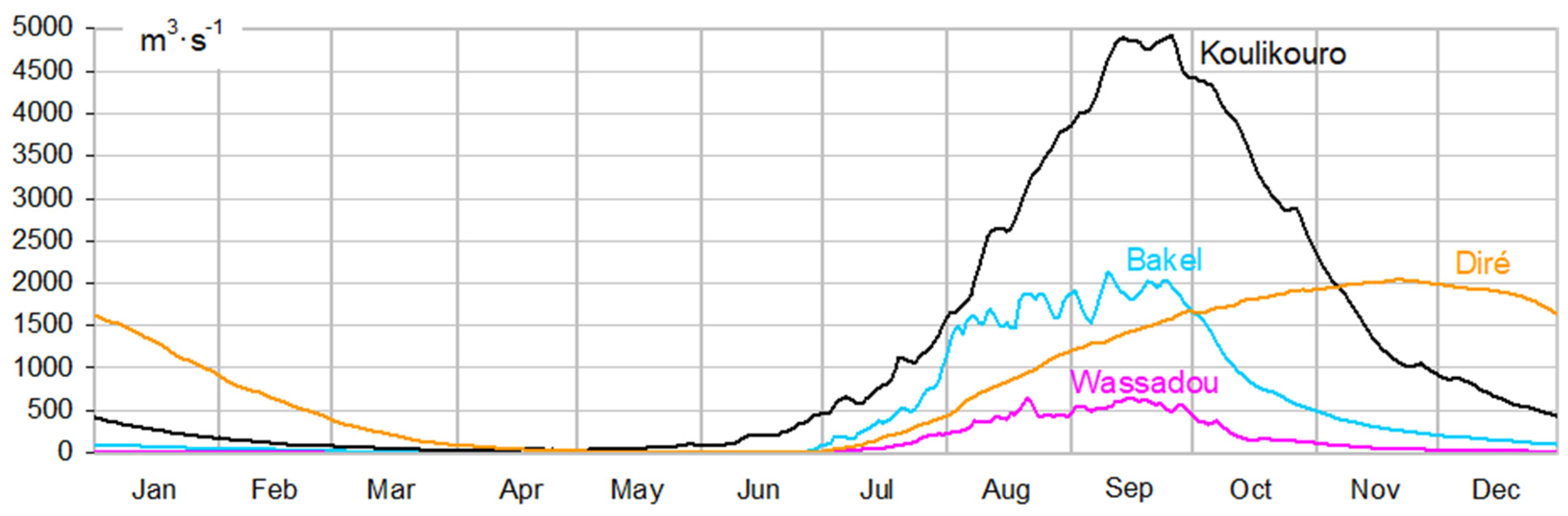
Figure 3.
Relationship between D (time elapsed since 15 September) and K at Daka Saidou on the Bafing (row 8; N = 10,966 observed values from 5 october 1952 to 20 october 2016; CNSE0 = 0.347 for model 1 with K = f(D), CNSE0 = 0.296 for model 3 with K = fb(D)).
Figure 3.
Relationship between D (time elapsed since 15 September) and K at Daka Saidou on the Bafing (row 8; N = 10,966 observed values from 5 october 1952 to 20 october 2016; CNSE0 = 0.347 for model 1 with K = f(D), CNSE0 = 0.296 for model 3 with K = fb(D)).

Figure 4.
Relationship between discharge Q and K at Daka Saidou on the Bafing (row 8; 10,966 points observed from 5 october 1952 to 20 october 2016; CNSE0 =0.392 for model 2 with K = g(Q); CNSE0 = 0.335 for model 4 with K = gb(Q)), with abscissa in logarithmic values on the left (a) and natural values on the right (b).
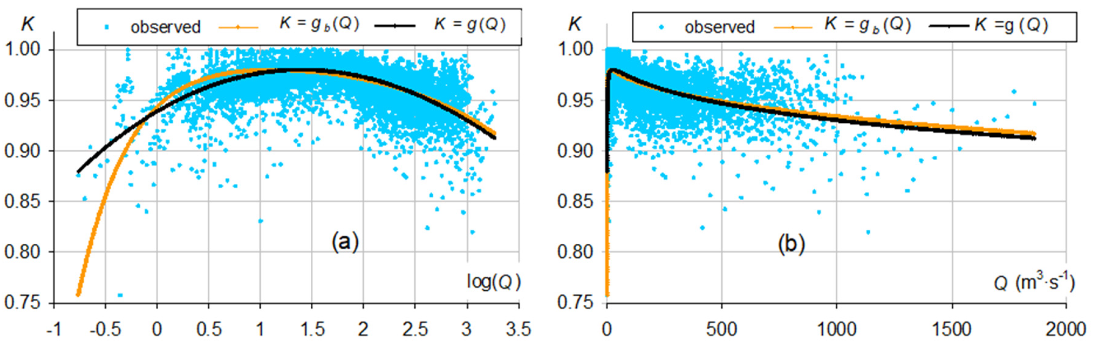
Figure 5.
Efficiency coefficient CNSE0 and number N of calibration of models 1 to 4 describing K as a function of D or Q, for each station analyzed.
Figure 5.
Efficiency coefficient CNSE0 and number N of calibration of models 1 to 4 describing K as a function of D or Q, for each station analyzed.

Figure 6.
Model 1 representing K as a function of the time D elapsed since the previous 15 September (K = f(D)) at the 54 stations located in the Senegal, Gambia and Niger basins, by sub-basins: High Bafing (a); Bafing (b); Faleme (c); Bakoye (d); Senegal (e); Gambia tributaries (f); Gambia (g); High Niger (h); Bani (i); Niger (j).

Figure 7.
Model 2 representing K as a function of the specific discharge Qs at the 25 stations located in the Senegal basin (relations K = g(Q)), with abscissa in logarithmic values on the left (index 1) and natural values on the right (index 2), by sub-basins: High Bafing (a1,a2), Bafing (b1,b2), Faleme (c1,c2), Bakoye (d1,d2), Senegal (e1,e2).

Figure 8.
Model 2 representing K as a function of the specific discharge Qs or the discharge Q at stations 26 to 54 in the Gambia and Niger basins (relations K = g(Q)), with abscissa in logarithmic values on the left (index 1) and natural values on the right (index 2), by sub-basins: Gambia tributaries (a1,a2), Gambia (b1,b2), High Niger (c1,c2), Bani (d1,d2), Niger (e1,e2).

Figure 9.
Mean Km of K observed and optimal value K0 maximizing the efficiency coefficient CNSE2 of the Nt discharge forecasts made with model 0 (Maillet) at horizons H between 1 and 120 days.
Figure 9.
Mean Km of K observed and optimal value K0 maximizing the efficiency coefficient CNSE2 of the Nt discharge forecasts made with model 0 (Maillet) at horizons H between 1 and 120 days.

Figure 10.
CNSE2 efficiency coefficient and number Nt of the discharge forecasts made with the different K models (optimal K0 value or D or Q functions) at all H horizons between 1 and 120 days.
Figure 10.
CNSE2 efficiency coefficient and number Nt of the discharge forecasts made with the different K models (optimal K0 value or D or Q functions) at all H horizons between 1 and 120 days.

Figure 11.
Performance of models in forecasting discharge during recession periods at Daka Saidou on the Bafing, according to the forecast horizon.
Figure 11.
Performance of models in forecasting discharge during recession periods at Daka Saidou on the Bafing, according to the forecast horizon.
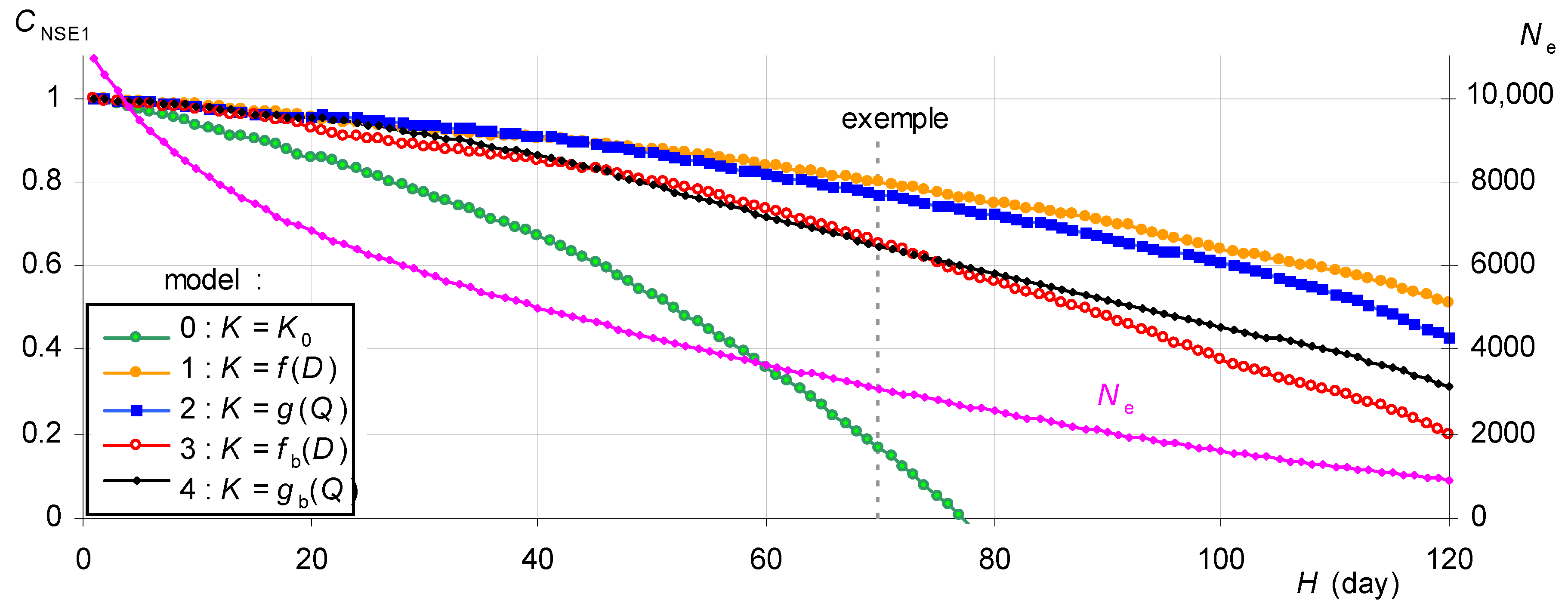
Figure 12.
Average model performance in forecasting discharge at all stations, according to the forecast horizon H (average of the relative standard error Rrmse, calculated on the Ns stations for which the number Ne of discharge forecasts at horizon H is greater than 1).
Figure 12.
Average model performance in forecasting discharge at all stations, according to the forecast horizon H (average of the relative standard error Rrmse, calculated on the Ns stations for which the number Ne of discharge forecasts at horizon H is greater than 1).
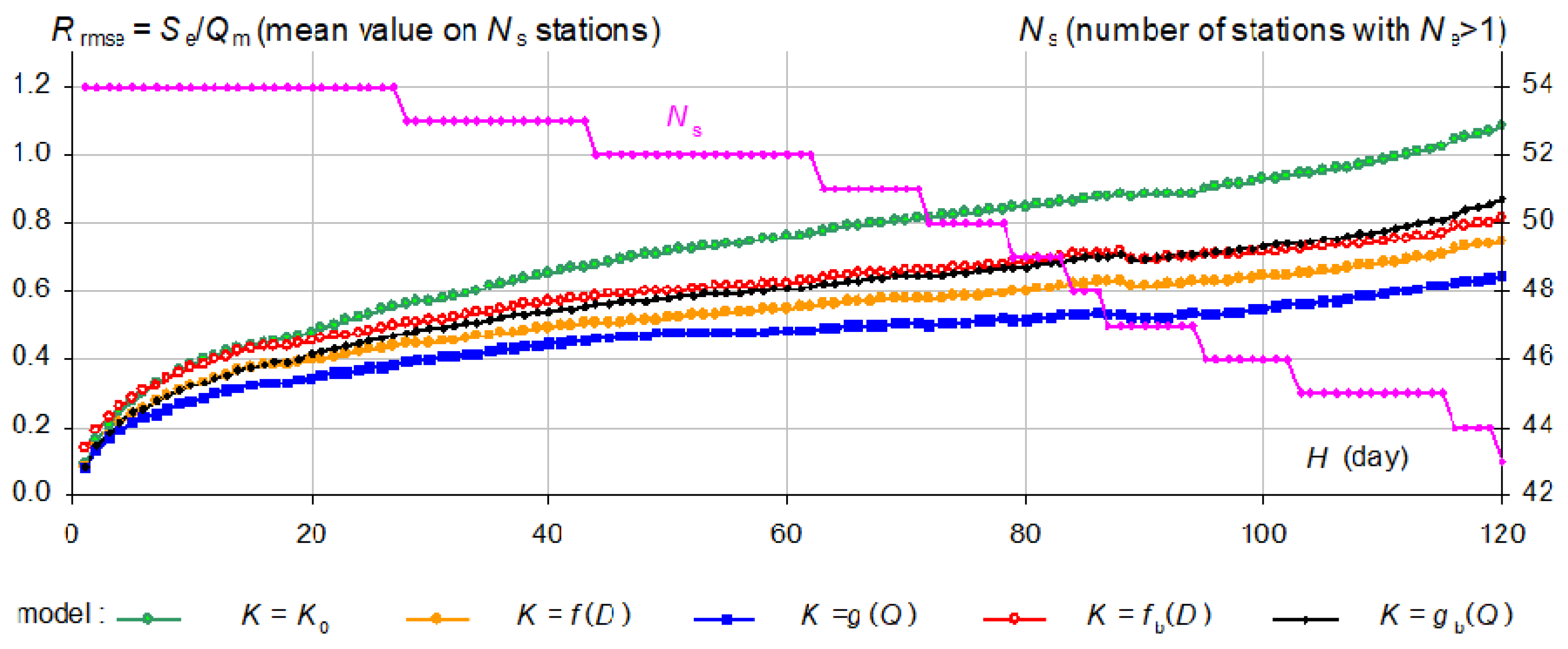
Figure 13.
Chronological evolution of the cumulative error Ce of model 2 with respect to the N = 10,966 observed values of K on the Bafing at Daka Saidou, for low flows with frequency of exceedance between 0.5 and 0.99 (a), high flows with frequency between 0.01 and 0.5 (b), and all flows except extreme flows, with frequency between 0.01 and 0.99 (c).

Figure 14.
Model 2 representing K as a function of discharge Q, calibrated on successive periods 1 to 3 and on the overall period, for the Bafing at Daka Saidou (station 8), with abscissa in logarithmic values on the left (a) and natural values on the right (b).
Figure 14.
Model 2 representing K as a function of discharge Q, calibrated on successive periods 1 to 3 and on the overall period, for the Bafing at Daka Saidou (station 8), with abscissa in logarithmic values on the left (a) and natural values on the right (b).

Figure 15.
Division of the data series into successive periods for each station, based on the dates of change in the overall slope of the time accumulation Ce of the model 2 error.
Figure 15.
Division of the data series into successive periods for each station, based on the dates of change in the overall slope of the time accumulation Ce of the model 2 error.
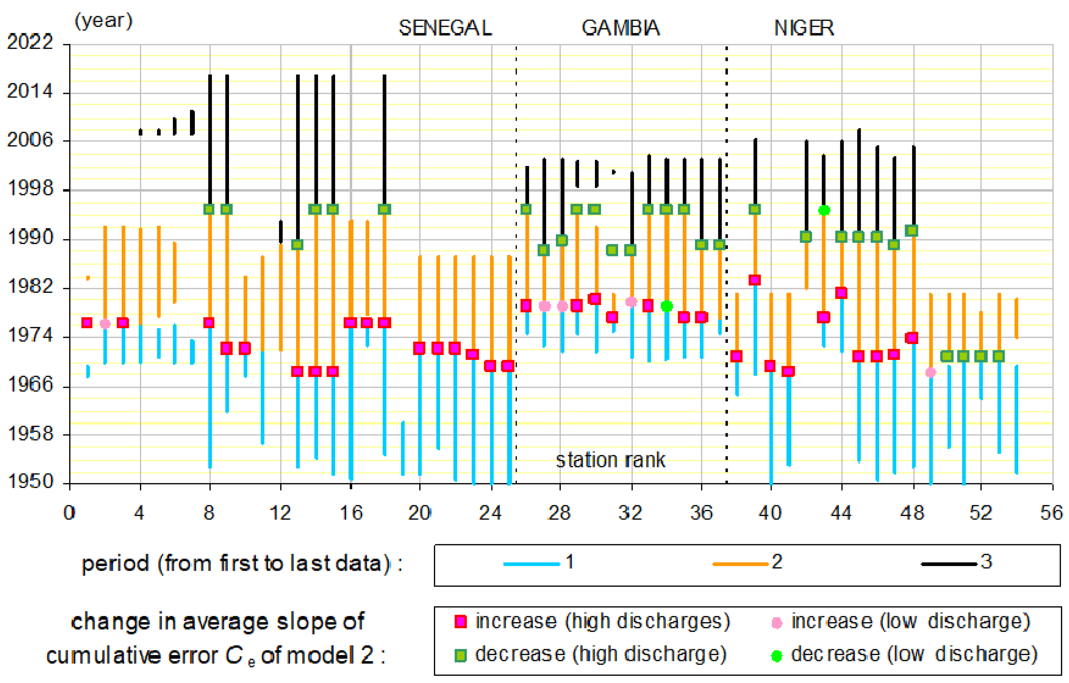
Figure 16.
Mean Km of K observed over each period 1 and 2 and minimum and maximum values of K modeled as a function of discharge (model K = g(Q) calibrated on all observations).
Figure 16.
Mean Km of K observed over each period 1 and 2 and minimum and maximum values of K modeled as a function of discharge (model K = g(Q) calibrated on all observations).


Table 1.
Senegal basin-list of stations analyzed, with their catchment area and mean specific discharge Qsm over the period 1970–1979.
Table 1.
Senegal basin-list of stations analyzed, with their catchment area and mean specific discharge Qsm over the period 1970–1979.
| Sub-Basin | River | Station | Rank | Long. (° W) | Lat. (° N) | Area (km2) | Qsm l·s−1·km−1 |
|---|---|---|---|---|---|---|---|
| High Bafing | Bafing | Pont km17 | 1 | 12°09′ | 10°29′ | 18 | 17.45 |
| High Bafing | Samenta | Doureko | 2 | 11°42′ | 11°18′ | 225 | 17.38 |
| High Bafing | Kioma | Teliko | 3 | 11°53′ | 11°22′ | 360 | 17.34 |
| High Bafing | Kioma | Salouma | 4 | 11°42′ | 11°17′ | 775 | 15.96 |
| High Bafing | Téné | Bebele | 5 | 11°49′ | 11°01′ | 3470 | 17.59 |
| High Bafing | Bafing | Balabori | 6 | 11°22′ | 11°18′ | 11,600 | 13.29 |
| Bafing | Bafing | Boureya | 7 | 10°44′ | 11°45′ | 14,800 | 12.77 |
| Bafing | Bafing | Daka Saidou | 8 | 10°37′ | 11°57′ | 15,700 | 12.50 |
| Bafing | Bafing | Makana | 9 | 10°17′ | 12°33′ | 22,000 | 10.44 |
| Bafing | Bafing | Soukoutali | 10 | 10°25′ | 13°12′ | 27,800 | 9.11 |
| Bafing | Bafing | Dibia | 11 | 10°48′ | 13°14′ | 33,500 | 7.74 |
| Faleme | Faleme | Moussala | 12 | 11°18′ | 12°31′ | 3103 | 10.04 |
| Faleme | Faleme | Fadougou | 13 | 11°23′ | 12°31 | 9300 | 5.75 |
| Faleme | Faleme | Gourbassy | 14 | 11°38′ | 13°24′ | 17,100 | 5.01 |
| Faleme | Faleme | Kidira | 15 | 12°13′ | 14°27′ | 28,900 | 3.61 |
| Bakoye | Bakoye | Toukoto | 16 | 09°53′ | 13°27′ | 16,500 | 2.94 |
| Bakoye | Baoule | Siramakana | 17 | 09°53′ | 13°35′ | 59,500 | 0.56 |
| Bakoye | Bakoye | Oualia | 18 | 10°23′ | 13°36′ | 84,700 | 1.05 |
| Bakoye | Bakoye | Kalé | 19 | 10°39′ | 13°43′ | 85,600 | 1.05 |
| Senegal | Senegal | Galougo | 20 | 11°03′ | 13°51′ | 128,400 | 2.79 |
| Senegal | Senegal | Gouina | 21 | 11°06′ | 14°00′ | 128,600 | 2.83 |
| Senegal | Senegal | Kayes | 22 | 11°27′ | 14°27′ | 157,400 | 2.32 |
| Senegal | Senegal | Bakel | 23 | 12°27′ | 14°54′ | 218,000 | 2.36 |
| Senegal | Senegal | Matam | 24 | 13°15′ | 15°39′ | 230,000 | 1.99 |
| Senegal | Senegal | Kaédi | 25 | 13°30′ | 16°08′ | 253,000 | 1.53 |
Table 2.
Gambia basin—list of stations analyzed, with their catchment area and mean specific discharge Qsm over the period 1970–1979.
Table 2.
Gambia basin—list of stations analyzed, with their catchment area and mean specific discharge Qsm over the period 1970–1979.
| Sub-Basin | River | Station | Rank | Long. (° W) | Lat. (° N) | Area (km2) | Qsm l·s−1km−1 |
|---|---|---|---|---|---|---|---|
| tributaries | Sili | pont routier | 26 | 12°16′ | 13°32′ | 90 | 9.12 |
| tributaries | Diarha | pont routier | 27 | 12°37′ | 12°36′ | 760 | 10.00 |
| tributaries | Tiokoye | pont routier | 28 | 12°32′ | 12°34′ | 950 | 9.41 |
| tributaries | Diaguery | pont routier | 29 | 12°05′ | 12°38′ | 1010 | 7.52 |
| tributaries | Niokolokoba | pont routier | 30 | 12°44′ | 13°04′ | 3000 | 2.65 |
| tributaries | Koulountou | Gué (parc) | 31 | 13°29′ | 12°47 | 5350 | 4.88 |
| tributaries | Koulountou | Missira Gounasse | 32 | 13°37′ | 13°12′ | 6200 | 5.13 |
| Gambia | Gambia | Kedougou | 33 | 12°11′ | 12°33′ | 7550 | 10.69 |
| Gambia | Gambia | Mako | 34 | 12°21′ | 12°52′ | 10,450 | 8.86 |
| Gambia | Gambia | Simenti | 35 | 13°18′ | 13°02′ | 20,500 | 6.42 |
| Gambia | Gambia | Wassadou amont | 36 | 13°22′ | 13°21′ | 21,200 | 6.20 |
| Gambia | Gambia | Wassadou aval | 37 | 13°23′ | 13°21′ | 33,500 | 3.96 |
Table 3.
Niger basin—list of stations analyzed, with their catchment area and mean specific discharge Qsm over the period 1970–1979.
Table 3.
Niger basin—list of stations analyzed, with their catchment area and mean specific discharge Qsm over the period 1970–1979.
| Sub-Basin | River | Station | Rank | Long. (° W) | Lat. (° N) | Area (km2) | Qsm l·s−1km−1 |
|---|---|---|---|---|---|---|---|
| High Niger | Sankarani | Selingue | 38 | 08°13′ | 11°38′ | 34,200 | 9.51 |
| High Niger | Niger | Banankoro | 39 | 08°40′ | 11°41′ | 70,740 | 12.72 |
| High Niger | Niger | Koulikouro | 40 | 07°33′ | 12°51′ | 120,000 | 10.60 |
| High Niger | Niger | Ke Macina | 41 | 05°21′ | 13°58′ | 141,000 | 8.41 |
| Bani | Degou | Manankoro | 42 | 07°27′ | 10°27′ | 1550 | 5.52 |
| Bani | Banifing | Kolondieba | 43 | 06°51′ | 11°03′ | 3050 | 3.36 |
| Bani | Baoulé | Madina Diassa | 44 | 07°40′ | 10°47′ | 7880 | 6.60 |
| Bani | Baoulé | Dioila | 45 | 06°48′ | 12°31 | 32,500 | 3.25 |
| Bani | Bani | Douna | 46 | 05°54′ | 13°12′ | 101,600 | 2.73 |
| Bani | Bani | Beneny Kegny | 47 | 04°54′ | 13°23′ | 116,000 | 2.47 |
| Bani | Bani | Sofara | 48 | 04°05′ | 14°05′ | 125,400 | 1.96 |
| Niger | Niger | Mopti | 49 | 04°12′ | 14°30′ | 281,600 | 3.00 |
| Niger | Niger | Akka | 50 | 04°14′ | 15°24′ | - | - |
| Niger | Niger | Diré | 51 | 03°23′ | 16°16′ | - | - |
| Niger | Niger | Koryoumé | 52 | 03°01′ | 16°40′ | - | - |
| Niger | Niger | Tossaye | 53 | 00°35′ | 16°57′ | - | - |
| Niger | Niger | Ansongo | 54 | −00°30′ | 15°40′ | - | - |
© 2020 by the authors. Licensee MDPI, Basel, Switzerland. This article is an open access article distributed under the terms and conditions of the Creative Commons Attribution (CC BY) license (http://creativecommons.org/licenses/by/4.0/).
Share and Cite
MDPI and ACS Style
Bader, J.-C.; Dacosta, H.; Pouget, J.-C. Seasonal Variations of the Depletion Factor during Recession Periods in the Senegal, Gambia and Niger Watersheds. Water 2020, 12, 2520. https://doi.org/10.3390/w12092520
AMA Style
Bader J-C, Dacosta H, Pouget J-C. Seasonal Variations of the Depletion Factor during Recession Periods in the Senegal, Gambia and Niger Watersheds. Water. 2020; 12(9):2520. https://doi.org/10.3390/w12092520
Chicago/Turabian StyleBader, Jean-Claude, Honoré Dacosta, and Jean-Christophe Pouget. 2020. "Seasonal Variations of the Depletion Factor during Recession Periods in the Senegal, Gambia and Niger Watersheds" Water 12, no. 9: 2520. https://doi.org/10.3390/w12092520
Note that from the first issue of 2016, this journal uses article numbers instead of page numbers. See further details here.