A Quantile Mapping Method to Fill in Discontinued Daily Precipitation Time Series
by
 , ,
, ,
Manolis G. Grillakis
1,2,* ,
,
Christos Polykretis
1,2 ,
,
Stelios Manoudakis
2,
Konstantinos D. Seiradakis
2 and
Dimitrios D. Alexakis
1,2 1
Lab of Geophysical-Remote Sensing & Archaeo-environment, Institute for Mediterranean Studies, Foundation for Research and Technology Hellas, 74100 Rethymno, Crete, Greece
2
School of Environmental Engineering, Technical University of Crete, 73100 Chania, Crete, Greece
*
Author to whom correspondence should be addressed.
Water 2020, 12(8), 2304; https://doi.org/10.3390/w12082304
Submission received: 7 July 2020
/
Revised: 5 August 2020
/
Accepted: 13 August 2020
/
Published: 17 August 2020
(This article belongs to the Section Hydrology)
Abstract
:We present and assess a method to estimate missing values in daily precipitation time series for the Mediterranean island of Crete. The method involves a quantile mapping methodology originally developed for the bias correction of climate models’ output. The overall methodology is based on a two-step procedure: (a) assessment of missing values from nearby stations and (b) adjustment of the biases in the probability density function of the filled values towards the existing data of the target. The methodology is assessed for its performance in filling-in the time series of a dense precipitation station network with large gaps on the island of Crete, Greece. The results indicate that quantile mapping can benefit the filled-in missing data statistics, as well as the wet day fraction. Conceptual limitations of the method are discussed, and correct methodology application guidance is provided.
1. Introduction
The cornerstone of meteorological and climatological science is the quality of measurement of precipitation. Large instrumentation gaps occur due to network destruction (fires, wars) or technical limitations that dictate network reorganizations [1]. This is a difficult issue to tackle as there are legacy networks which provide decades of valuable data which, for various reasons, have been discontinued. An obvious workaround of treating missing values is to include only part of the data in the analyses, which however, may lead to the exclusion of valuable information from them or even induce unwanted biases [1]. Other methodological approaches to deal with the gaps is to fill in missing values using data from the same station (temporal fill-in of the missing data) or to make use of interpolation-based techniques that utilize nearby stations’ recordings to estimate the missing values (spatial fill-in) [2]. Temporal fill-in, however, has been found to be more suitable for variables with high autocorrelation and for calculating long-term averages and hence it is not suitable for daily precipitation [2]. Regarding the spatial interpolation methodologies found in the literature, they mainly belong to two major categories: geographical interpolation methods, which consider the location of the station, and non-geographical methods. Methods belonging in the first category among others are the kriging family of methods [3], while nearest neighbors, Thiessen polygons [4], and inverse distance weighting (IDW) [5] are classified as non-geographical methods [6]. Their main difference lies in the fact that geographical methods use the spatial correlation between neighboring observations to provide estimates of precipitation in the desired locations.
Many studies have tested the efficiency of interpolation methodologies in their ability to estimate the spatial fields of precipitation on different temporal scales, which can also be considered as a metric to assess the ability to fill in discontinuities. Despite the number of methods and the shakedown studies, the literature is not conclusive about the performance ranking of the different interpolation methods for the various timescales, showing that there are some usually well performing methods but with case-specific results. Regarding daily precipitation data fill-in, [7] tested ordinary kriging and co-kriging based methods of IDW were applied to interpolate daily precipitation in China. Co-kriging was found to provide better results compared to the other two methodologies, also indicating the drawbacks of IDW compared to geographical methods. In the same manner, one study [8] tested two interpolation methods, IDW and the multiquadric–biharmonic method, in a dense precipitation measuring network in the United States, indicating that the latter provided better results. In contrast to those findings, another author [9] studied a network of 13 rain gauges on Norfolk Island, finding that IDW and Thiessen methodology provided similar results compared to kriging. In a much broader study in terms of data for Northeast China [10], 40 years of data from 72 stations were studied, indicating similar results, i.e., that more complex methods did not provide added value compared to the simple IDW. In another study focused on a mountainous region of Israel [11], IDW methodology was shown to perform better compared to a local weighted regression (LWR) that also considered elevation and other explanatory variables. In coarser temporal precipitation resolution focused studies (monthly, annual), the comparison between different interpolation methodologies is not also conclusive. One study [12] compared ordinary kriging, IDW and splines to estimate annual precipitation, concluding that ordinary kriging performed better compared to the other two methods. It must be mentioned that the explicit characteristics of each case study region and its precipitation regime vary the attained comparison results. As an example, densely gauged case studies or regions with uniform precipitation characteristics (in space and/or time) are expected to aid simpler interpolation methods to perform well. However, in regions with sparse precipitation observations, the missing information can be complemented by secondary attributes that are more densely sampled [3]. Furthermore, in higher temporal resolution cases, i.e., daily data, the spatial variability of the precipitation may be so large that the theoretical advantage of more sophisticated methods may be diminished. In general, it can be said that the spatial variability of the precipitation increases as the timescale decreases; hence, regardless of the interpolation methodology, the skill is expected to increase as the timescale becomes larger. This highly stochastic nature of precipitation compared to other climatic variables such as temperature has also been mentioned [13]. Adding to the above-mentioned methodologies, also data-driven approaches have been used in the literature to fill in precipitation data. Indicative examples are the use of artificial neural networks to fill missing data form nearby stations [14,15].
Noteworthy drawbacks of the weighting and regression methods for daily precipitation fill-in are the overestimation of the number of rainy days, as they combine the rainy days of many nearby stations, as well as the distortion of the rainfall probability distribution, with heavy precipitation events likely to be systematically underestimated [1]. As a result, a side effect of the spatial fill-in procedures is that the estimated precipitation values most likely do not follow the statistical properties of the site. Beyond the under or over-estimation of the precipitation values, the probability distribution would be hampered. In this direction, quantile mapping-based methods have been used to adjust the statistical properties of the filled-in values. One study [16] used quantile mapping (QM) with empirical cumulative distribution function to fill in daily precipitation data voids over the Northwest Himalayas. The authors directly used the mapping of missing precipitation measurements from one station to another station and compared to the other simpler fill-in methodologies, finding that QM provided the best results. Similarly, another study [1] presented a methodology to estimate missing daily precipitation data that uses quantile mapping based on the gamma distribution function, in combination with multiple linear regression.
In this work, we present a method to fill in missing values in daily precipitation series that is tested and applied on the Mediterranean island of Crete. On the island, there have been two major legacy networks gauging daily precipitation. The development of the methodology presented in this work was motivated by the need to fill in each network’s gaps. The methodology is based on a two-step procedure: (a) assessment of the values from nearby stations and (b) adjustment of the biases in the probability density function of the filled values towards the target point of existing data. A set of different approaches for step (a) are considered and exhaustively tested. The results are meticulously tested using subsampling cross-validation.
2. Materials and Methods
2.1. Case Study Region
The island of Crete covers more than 6% of the area of Greece and is the 5th largest Mediterranean island. Crete’s climate is characterized as dry sub-humid Mediterranean, exhibiting warm and dry summers while winters are cold and rainy. More than 40% of the annual precipitation occurs in the months of December to February. The average precipitation of the island ranges from 440 mm/year in the eastern part of the island to more than 2000 mm/year in the western mountainous regions. The island of Crete exhibits a steep terrain, with elevations as high as 2456 m a.s.l. The steep orography has a strong effect on the precipitation regimen, with large orographic precipitation effects to be observed [17,18,19,20] that, in combination with its location within the Mediterranean, have resulted in numerous heavy precipitation events that were followed by serious flooding events, such as those which occurred in the Giofiros region in 1994 [17,21], in the Almirida region in 2007 [22,23], as well as February 2019′s extensive flooding in the Chania prefecture [24] and floods in the southern parts of the island [25]. Recent findings have indicated that the region’s precipitation regime facilitates rainfall induced soil erosivity to a larger extend than was previously thought [26,27]. From a hydrogeological perspective, the island is mainly composed of pre-alpine and alpine carbonate formations and neogene and quaternary (alluvial) sediments which expedite water penetration; hence, the region exhibits limited surface water resources [28]. Crete is a well-studied region in the context of climate change impacts, mainly for its location and size, its environmental heterogeneity, but also due to its hydrological isolation from continental Greece, which makes it ideal for studying climate change impacts [21,29,30,31].
2.2. Precipitation Data Availability
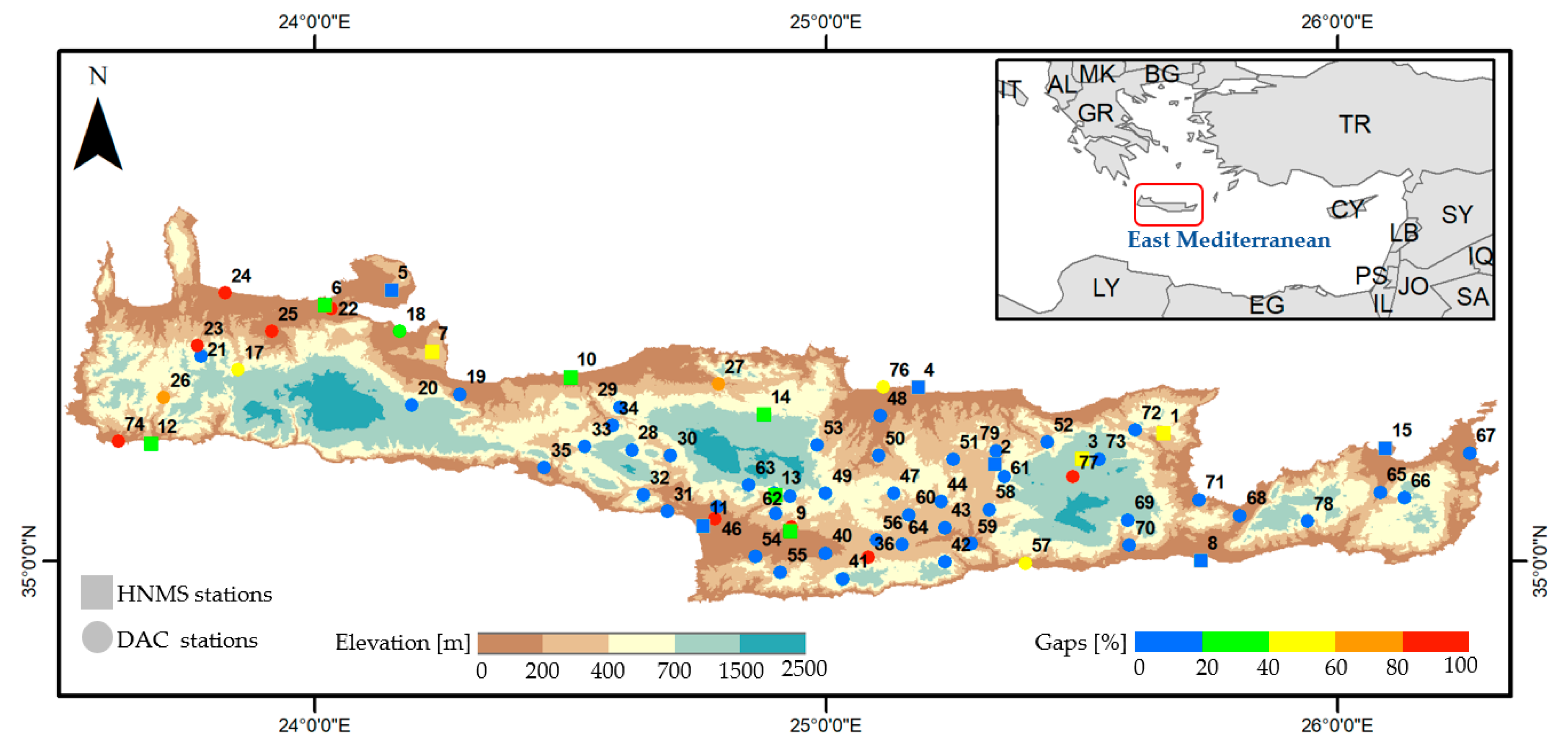
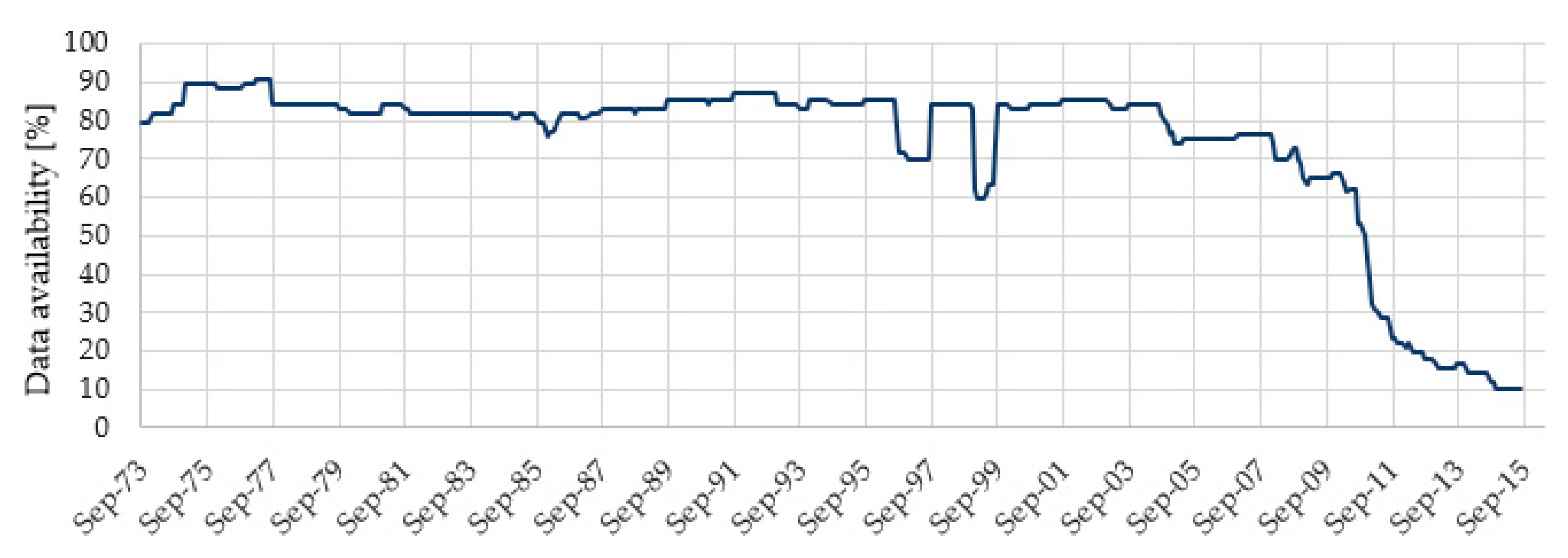
On the island of Crete, there have been two major precipitation gauging station networks. The first one has been in service since the early 1970s and was operated by the Decentralized Administration of Crete (DAC) (formerly Prefecture of Crete), from which data are mostly available from the period between 1973 and 2015, collected by a total of 62 stations. The second network of 15 stations is being operated by the Hellenic National Meteorological Service (HNMS), which has largely ceased operation, but some of the stations are still in operation. In recent years, another fully automatic network of meteorological stations has been developed from the National Observatory of Athens (NOA), but it is not assessed in this study due to the very few stations that provide data for periods longer than 10 years. The spatial distribution of the two networks, as well as the overall gaps of each station, are shown in Figure 1. In Figure 2, the temporal availability is shown, with 100% corresponding to all 77 stations that were considered. As can be observed, prior to 2008, the availability of the data ranged between 70% and 90%, while there was a gradual decrease in recent years, with the year 2015 having an availability of ~10% (8 stations).
2.3. Methodology
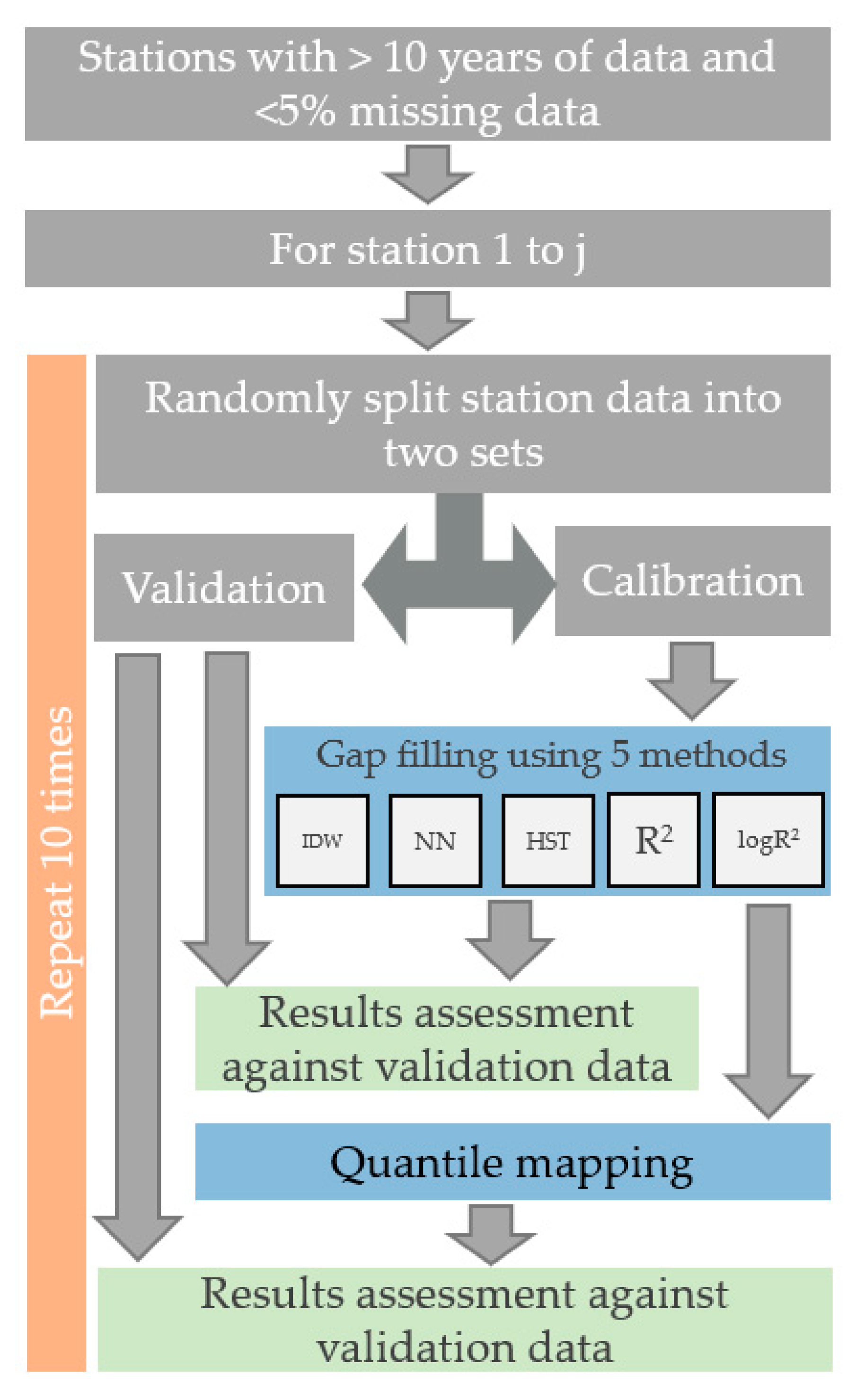
The methodology is divided into two discrete processing steps. First, the gaps are filled in in a spatial manner. Five different methods were assessed, including non-geographical interpolation techniques. After the fill-in, as a second step, the cumulative density function (CDF) of the filled-in values is adjusted towards the already existing data on the station. The two steps are analyzed in detail. To effectively assess the performance of the two-step procedure and the different methods, we considered all the stations that provide data for at least 10 years and with at least 95% completeness of daily data in each year. To assess the methods, we obtained data from one station at a time, randomly split the available data into a calibration and validation set and applied the two-step fill-in methodology. The validation portion of the data was considered to be the gaps that needed to be filled in. The results of the fill-in procedure were then assessed against the validation set. The procedure was repeated 10 times per station to ensure that the random split of the data into calibration and validation sets did not affect the results. This number was considered to be sufficient for the experimental design needs, as in the literature, similar calibration validation schemes are found to use six [32] to twenty [33] permutations. A flowchart with the procedure followed is shown in Figure 3.
2.3.1. Gap Filling
Five different methods of spatially filling the (artificially made) missing values were assessed. These are as follows: (a) the inverse distance weighting (IDW) method [5] (with a distance power of 2), (b) the spatially nearest station, (c) the least histogram distance, (d) the station with the best coefficient of determination (R2) [34] between the concurrent daily values and (e) the station with the best R2 as determined in (d), estimated from the logarithm of precipitation values. Method (a), IDW, is the only one that exploits multiple values of the nearby stations to estimate a missing value on the target station. The remaining four are different methods of selecting a substituting value from a single station. The nearest station uses the Euclidean distance as a criterion to select the station from which to assess a missing value. As for the number of the utilized neighbor stations, all the stations that provide a precipitation value at each timestep were considered. The least histogram distance method (HST) compares the histograms between the existing data of the target station and other stations explicitly. The histogram assessment was performed using a bin size of 1 mm. The distance of the histograms was quantified by estimating the root mean squared difference. Method (d) estimates the R2 between the existing data of the target station and other stations explicitly, and each missing value on the target station is substituted with the available precipitation value from the station with the best R2. Method (e) is the same as (d), with the difference being that the R2 is estimated from the logarithm (base of 10) of the precipitation. This methodology is routinely used in hydrological model assessment along with the Nash–Sutcliffe criterion [35]. The logarithmic transformation of the precipitation helps to flatten the rarer high values, while lower precipitation values are comparatively retained. Hence, the sensitivity of R2 to the high precipitation values is mitigated. It has to be mentioned that, in order to estimate the logarithmic value of the precipitation, all the zero precipitation values were omitted.
2.3.2. Quantile Mapping Correction
The filled-in data of a station using the abovementioned methods are then adjusted in their CDF using the existing observed data. The methodology used here is multi-segment statistical bias correction (MSBC) [36]. This method belongs to the wider family of quantile mapping techniques. The method considers discrete segments of the cumulative density function space and applies quantile mapping correction in each segment individually. A step by step example of applying the multi-segment correction methodology is provided elsewhere [32,36]. The methodology has proven to be efficient to adjust daily climate model data in a number of local [20,37,38,39] and global scale studies [39,40]. The methodology considers a wet day fraction adjustment before the quantile mapping, by adjusting the usually excessive wet days of the climate model simulations to the observed one. A threshold of 0.1 mm per day was considered for the wet day definition. Technical details about the application of the method are provided in the Appendix A in [36].
2.3.3. The Effect of the Ratio between the Filled in Data and the Existing Data
The previously described methodology quantifies the effect of quantile mapping on the fill-in data post-processing, under the assumption that the gaps to be filled are equal to the available data on the specific location. This has an important methodological implication for the quantile mapping application: when the filled gaps are much less (or much more) than the available data, the quantile mapping tends to stretch the filled values to cover the entire CDF space of the existing observations. Hence, it tends to inflate (or deflate) some of the frequent and low (or, more rarely, high) precipitation values to represent high return period events (milder events). On the above described experimental design, the gaps were considered equal to the existing data length, while also the length of the gaps/existing data were at least 10 years (5 years each), which allowed for a reasonable climate sampling. To quantify the effect of the total number of gaps to be filled in, an experiment was conducted in which the artificially created gaps varied between 20% and 90%.
3. Results and Discussion
3.1. Gap Filling Methods Assessment
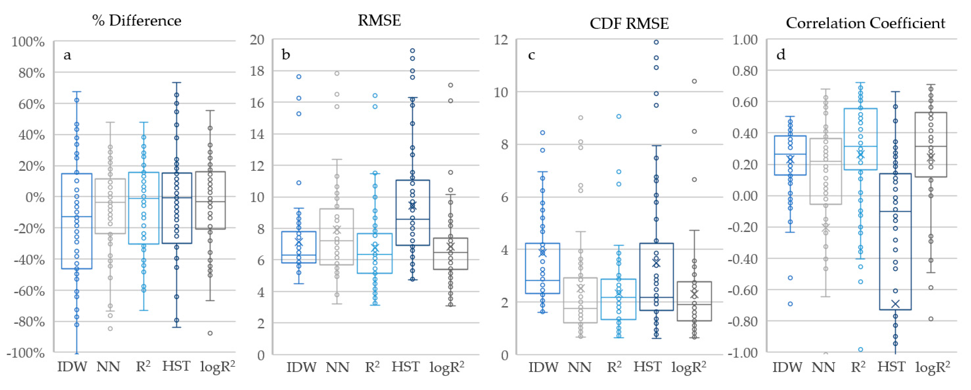
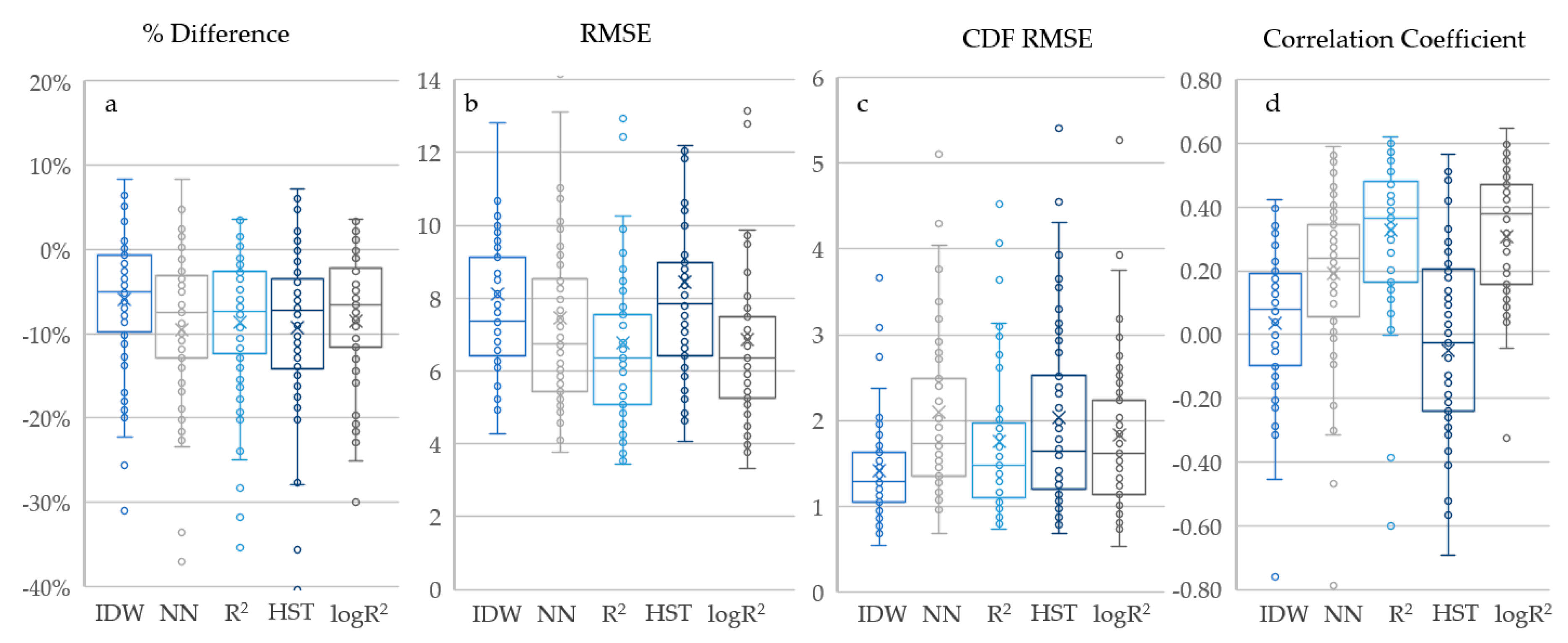
The results of the different methods to fill in the gaps are assessed in this section. Figure 4 shows the results of the comparison between the different gap filling methods against the validation data. Each dot in the boxplots corresponds to the results of each station omitted from validation. As the procedure was repeated 10 times, each point is the average among the 10 experiment permutations. Quantitatively, the % differences are remarkably high and mainly range between −40% and 20%. The RMSE of all methods ranges between 5 and 12 mm. The comparison between the ranked (CDF) values show better agreement than expected, with RMSE mainly between 1 mm and 5 mm. The Pearson’s correlation coefficient varies highly among the different methods, between −0.8 and 0.8. In terms of % difference, NN and logR2 methods are better at filling in data. The R2 and logR2 exhibit low root mean squared error (RMSE), while HST shows poor results. When the CDF of the filled-in data is compared to the validation data’s CDF, the NN, R2 and logR2 show better performance. Finally, in terms of Pearson’s correlation coefficient, the R2 and logR2 show the best results.
3.2. Benefits of Quantile Mapping
In Figure 5, we compare the different fill-in methods’ results to the validation data after the application of the quantile mapping. The benefits of the different metrics are profound. After the quantile mapping, all filling-in methods show a percent difference mainly between −15% and 0%, largely improving the difference, even with remaining negative bias (constructed precipitation values are lower than the actual validation values). The RMSE shows limited improvement, but in terms of CDF RMSE, the improvement signal is clearer, with RMSE values ranging between 1 mm and 3 mm. In terms of Pearson’s correlation coefficient, the results are roughly similar or even degraded compared to the non-quantile mapping application. An important point to be mentioned is that, while quantile mapping improved some aspects of the fill-in process, it did not significantly change the relative performance among the different fill-in methods. Hence, from a fill-in point of view, the best performing method is the R2, which provides a reasonable % difference, with the lowest RMSE, the second best RMSE in the CDF comparison and one of the best performing correlation coefficients.
3.3. Wet Day Fraction Adjustment
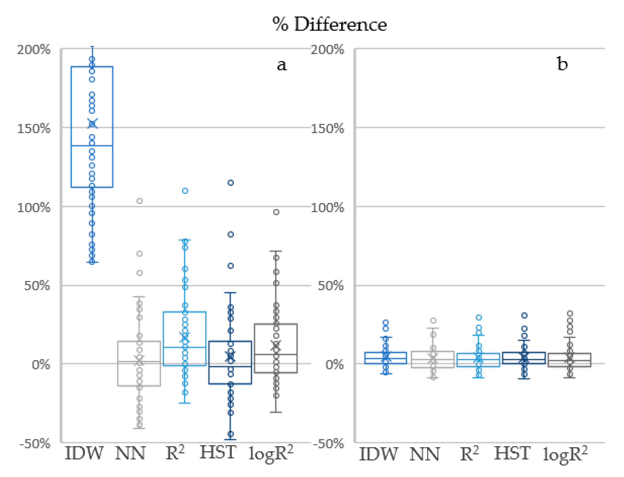
Beyond the benefits of the quantile mapping for the statistics of the filled-in data, the effect of the wet day fraction adjustment was assessed. In Figure 6, the difference in the wet day fraction in the filled-in values was assessed before and after the adjustment. The results indicate that the IDW driven fill-in methods result in a major wet day overestimation (Figure 6a). This result does not come as a surprise, as the IDW is the only technique tested that considers the combination of data from various nearby stations. The rest of the methods seem to exhibit a more limited difference in the wet day fraction, yet this is still high enough. This confirms the large discrepancy that may be exhibited between nearby stations as a result of the complex terrain and the uniformity of the microclimatic conditions of the island. The wet day correction applied provides a considerable improvement in the results, as shown in Figure 6b. The mostly positive remaining difference that all the fill-in methods exhibit is explained by the methodology of the wet day correction, i.e., the wet days of the filled-in values are trimmed to fit the observed data of the station. However, in the opposite case, i.e., filled-in data exhibit smaller fraction of wet days, the methodology (originally designed to work on climate model data) does not perform any adjustments.
3.4. The Effect of the Gap Size Relative to the Already Available Data on the Station
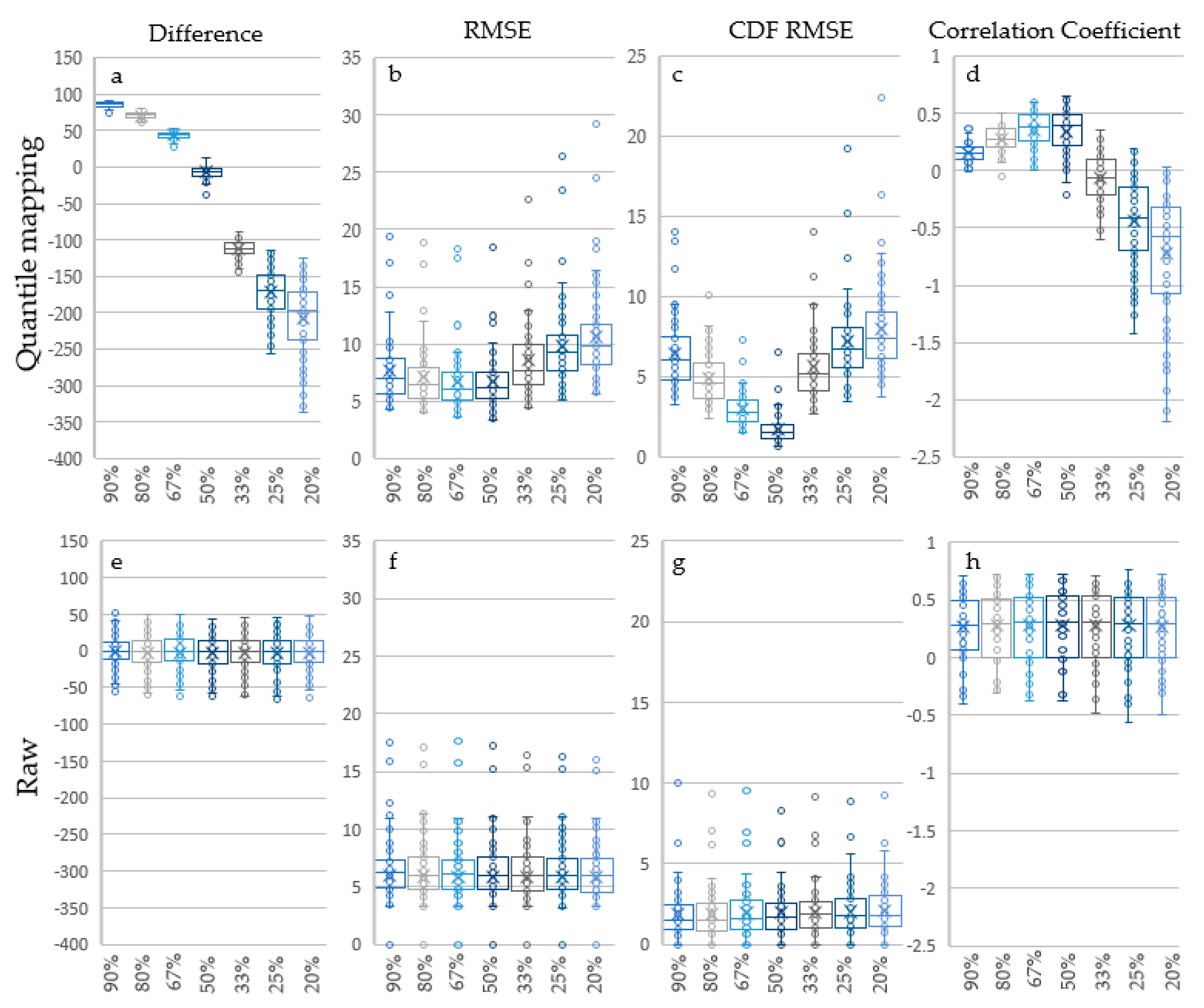
In this section, the results of the experiment described in Section 2.3.3 are presented. In order to quantify the effect of the total number of gaps to be filled-in compared to the already existing amount of data, we repeated the previous analysis (only for the R2 gap filling method), this time modifying the % of the artificially created gaps. Again, ten repetitions of the experiment were used. The results of the quantile mapping are shown in Figure 7a–d against the same experiment’s results with only the fill-in procedure (Figure 7e–h). It is shown that, in all the estimated metrics, the best attained results were found for gap sizes equal to the available observation of the station. The performance of all the metrics, i.e., the % difference, the RMSE, the RMSE of the CDF and the correlation coefficient, deteriorates beyond and below the ratio one to one between the gaps and the available data. In contrast, the results of the experiments without quantile mapping show an invariability with the fraction of the gaps that were filled in. All the above suggest that, when the gap size is different to the already existing data, then (a) when the gaps are less than the already existing data on the station, the quantile mapping of the same data length should be considered, even if the data are already known, and (b) in the opposite case when the gaps are more than the available data, then the gaps should be bias adjusted in batches similar to the available data length.
4. Discussion and Conclusions
A method to adjust the filled-in missing data of daily precipitation measurements is presented. The methodology is applied and tested for the Mediterranean island of Crete. The methodology makes use of a quantile mapping bias correction technique originally designed for daily precipitation adjustment in climate models. The methodology was tested on a large number of stations by creating artificial data gaps that were filled-in and processed with the presented methodology. The results were assessed using a subsampling cross-validation technique. The analysis performed suggests that the methodology works best when the gaps are filled in using the data of most similar station in terms of R2. Furthermore, experimental evidence provided here shows that the ratio of the missing data to the available data on the specific station of interest is a very important parameter that should be taken into consideration when this methodology is applied. The presented results indicate that quantile mapping offers profound benefits to the fill-in procedure, even if it does not benefit all aspects of the statistics. The large improvement in the difference and the CDF statistics shows that the quantile mapping adds value to the data, mainly when the filled-in data are used for long-term analyses rather than the reconstruction of a single precipitation event, even though, in the latter case, quantile mapping does not seem to statistically deteriorate the precipitation statistics. Further improvements could be achieved if the methodology was able to adjust the wet day fraction, even when the filled-in wet day fraction was lower than the respective fraction of the existing data on the specific station. The methodology could benefit the fill-in of other climatic variables under the condition that an appropriate quantile mapping methodology is used. As an example, the temperature variable cannot be processed with quantile mapping with the gamma distribution function as it cannot facilitate negative values. A drawback of this study is that this methodological sequence has not yet been tested for other regions; hence, its applicability elsewhere, outside the island of Crete, cannot be guaranteed.
Author Contributions
Conceptualization, M.G.G. and D.D.A.; methodology, M.G.G., C.P., S.M., K.D.S., D.D.A.; formal analysis, M.G.G., C.P., S.M., K.D.S.; investigation, M.G.G., C.P., S.M., K.D.S., D.D.A.; resources, D.D.A.; data curation, M.G.G.; writing—original draft preparation, M.G.G.; writing—review and editing, C.P., S.M., K.D.S., D.D.A.; visualization, M.G.G., C.P., S.M., K.D.S., D.D.A.; funding acquisition, D.D.A. All authors have read and agreed to the published version of the manuscript.
Funding
This research is part of a project which has received funding from the Hellenic Foundation for Research and Innovation (HFRI) and the General Secretariat for Research and Technology (GSRT), under grant agreement no. 651.
Acknowledgments
We acknowledge the Hellenic National Meteorological Service (HNMS) and Decentralized Administration of Crete for providing the data that were used in this study.
Conflicts of Interest
The authors declare no conflict of interest.
Appendix A

Table A1.
Location and information about the precipitation stations used in this study.
| Map ID | Name | Code | Elev (m) | Lon (deg) | Lat (deg) | Operated by | Gaps (%) |
|---|---|---|---|---|---|---|---|
| 1 | Fourni | MT54 | 316 | 25.7 | 35.3 | HNMS | 40.9 |
| 2 | Kasteli | MT50 | 349 | 25.3 | 35.2 | HNMS | 8.3 |
| 3 | Tzermiades | RG9 | 820 | 25.5 | 35.2 | HNMS | 53.3 |
| 4 | Herakleio | MT18 | 39 | 25.2 | 35.3 | HNMS | 0.0 |
| 5 | Souda | MT52 | 148 | 24.2 | 35.5 | HNMS | 0.0 |
| 6 | Chania | MT55 | 151 | 24 | 35.5 | HNMS | 25.6 |
| 7 | Vamos | MT51 | 240 | 24.2 | 35.4 | HNMS | 47.6 |
| 8 | Ierapetra | MT17 | 18 | 25.7 | 35 | HNMS | 11.4 |
| 9 | Gortys | MT16 | 182 | 24.9 | 35.1 | HNMS | 28.4 |
| 10 | Rethymno | 5.1 | 24.5 | 35.4 | HNMS | 25.3 | |
| 11 | Tympaki | 6 | 24.8 | 35.1 | HNMS | 0.0 | |
| 12 | Palaiochora | 20 | 23.7 | 35.2 | HNMS | 35.4 | |
| 13 | Zaros | 350 | 24.9 | 35.1 | HNMS | 35.0 | |
| 14 | Anwgeia | MT49 | 740 | 24.9 | 35.3 | HNMS | 25.9 |
| 15 | Sitia | MT38 | 114.1 | 26.1 | 35.2 | HNMS | 0.0 |
| 16 | Prasses | RG29 | 520 | 23.9 | 35.4 | DAC | 57.1 |
| 17 | Kalyves | MT19 | 19.9 | 24.2 | 35.4 | DAC | 20.4 |
| 18 | Mouri | RG18 | 50 | 24.3 | 35.3 | DAC | 8.1 |
| 19 | Askyfou | RG4 | 740 | 24.2 | 35.3 | DAC | 14.9 |
| 20 | Palaia Roumata | RG20 | 316 | 23.8 | 35.4 | DAC | 15.5 |
| 21 | Agrokipio | MT3 | 8 | 24 | 35.5 | DAC | 85.7 |
| 22 | Zymbragou | MT46 | 235 | 23.8 | 35.4 | DAC | 90.5 |
| 23 | Tavronitis | MT41 | 15.4 | 23.8 | 35.5 | DAC | 86.7 |
| 24 | Alikianos | MT4 | 66.3 | 23.9 | 35.4 | DAC | 90.5 |
| 25 | Kantanos | MT21 | 465.8 | 23.7 | 35.3 | DAC | 75.5 |
| 26 | Garazo | MT47 | 260 | 24.8 | 35.3 | DAC | 67.2 |
| 27 | Gerakari | RG8 | 660 | 24.6 | 35.2 | DAC | 10.0 |
| 28 | Kavousi | RG14 | 580 | 24.6 | 35.3 | DAC | 15.1 |
| 29 | Vizari | RG25 | 310 | 24.7 | 35.2 | DAC | 16.7 |
| 30 | Ag. Galini | RG1 | 20 | 24.7 | 35.1 | DAC | 15.3 |
| 31 | Melampes | RG16 | 560 | 24.6 | 35.1 | DAC | 18.0 |
| 32 | Spili | MT39 | 390 | 24.5 | 35.2 | DAC | 19.3 |
| 33 | Voleones | RG26 | 260 | 24.6 | 35.3 | DAC | 18.8 |
| 34 | Leukogeia | MT28 | 90 | 24.4 | 35.2 | DAC | 12.5 |
| 35 | Sternes | RG23 | 300 | 25.1 | 35 | DAC | 90.5 |
| 36 | Zaros | MT45 | 500 | 24.9 | 35.1 | DAC | 10.1 |
| 37 | Morwni | RG17 | 400 | 24.9 | 35.1 | DAC | 0.0 |
| 38 | Lagolia | RG15 | 140 | 24.8 | 35.1 | DAC | 2.6 |
| 39 | Vagionia | RG24 | 190 | 25 | 35 | DAC | 12.7 |
| 40 | Kapetaniana | RG13 | 800 | 25 | 35 | DAC | 13.5 |
| 41 | Axentrias | RG5 | 680 | 25.2 | 35 | DAC | 14.1 |
| 42 | Kalyvia | RG12 | 200 | 25.2 | 35.1 | DAC | 12.5 |
| 43 | Partira | RG21 | 400 | 25.2 | 35.1 | DAC | 9.5 |
| 44 | Gortys | 180 | 24.9 | 35.1 | DAC | 81.0 | |
| 45 | Tympaki-YEB | MT43 | 20 | 24.8 | 35.1 | DAC | 88.1 |
| 46 | Metaksoxwri | MT31 | 430 | 25.1 | 35.1 | DAC | 9.1 |
| 47 | Foinikia | MT13 | 40 | 25.1 | 35.3 | DAC | 7.1 |
| 48 | Ag. Varvara | MT1 | 570 | 25 | 35.1 | DAC | 6.3 |
| 49 | Profitis Hlias | MT36 | 380 | 25.1 | 35.2 | DAC | 3.8 |
| 50 | Voni | MT44 | 330 | 25.2 | 35.2 | DAC | 10.9 |
| 51 | Avdou | MT9 | 230 | 25.4 | 35.2 | DAC | 15.5 |
| 52 | Krousswnas | MT27 | 500 | 25 | 35.2 | DAC | 11.3 |
| 53 | Pompia | MT35 | 150 | 24.9 | 35 | DAC | 12.9 |
| 54 | Ag. Kyrillos | MT2 | 450 | 24.9 | 35 | DAC | 11.9 |
| 55 | Asimi | MT8 | 200 | 25.1 | 35 | DAC | 13.1 |
| 56 | Kapsaloi | MT22 | 10 | 25.4 | 35 | DAC | 40.7 |
| 57 | Kasanos | MT24 | 320 | 25.3 | 35.1 | DAC | 11.5 |
| 58 | Demati | MT10 | 210 | 25.3 | 35 | DAC | 13.8 |
| 59 | Tefeli | MT42 | 360 | 25.2 | 35.1 | DAC | 4.8 |
| 60 | Armaxa | MT6 | 450 | 25.3 | 35.2 | DAC | 12.3 |
| 61 | Gergeri | MT15 | 450 | 24.9 | 35.1 | DAC | 7.1 |
| 62 | Vorizia | RG27 | 520 | 24.8 | 35.1 | DAC | 4.0 |
| 63 | Protoria | MT37 | 225 | 25.1 | 35 | DAC | 12.7 |
| 64 | Marwnia | MT30 | 150 | 26.1 | 35.1 | DAC | 17.9 |
| 65 | Katsidwni | MT25 | 480 | 26.1 | 35.1 | DAC | 10.5 |
| 66 | Palaikastro | RG19 | 25 | 26.3 | 35.2 | DAC | 16.1 |
| 67 | Paxeia Ammos | MT34 | 50 | 25.8 | 35.1 | DAC | 16.7 |
| 68 | Malles | MT29 | 590 | 25.6 | 35.1 | DAC | 9.5 |
| 69 | Mythoi | MT32 | 200 | 25.6 | 35 | DAC | 18.9 |
| 70 | Kalo Xwrio | MT20 | 20 | 25.7 | 35.1 | DAC | 6.2 |
| 71 | Neapoli | MT33 | 240 | 25.6 | 35.3 | DAC | 8.3 |
| 72 | Eksw Potamoi | RG6 | 840 | 25.5 | 35.2 | DAC | 15.6 |
| 73 | Kountoura | MT26 | 8.9 | 23.6 | 35.2 | DAC | 82.9 |
| 74 | Heraklio-YEB | RG11 | 15 | 25.1 | 35.3 | DAC | 54.8 |
| 75 | Ag. Gewrgios | RG2 | 850 | 25.5 | 35.2 | DAC | 90.5 |
| 76 | Stavroxwri | MT40 | 325 | 25.9 | 35.1 | DAC | 10.9 |
| 77 | Kasteli-YEB | MT23 | 350 | 25.3 | 35.2 | DAC | 12.7 |
References
- Simolo, C.; Brunetti, M.; Maugeri, M.; Nanni, T. Improving estimation of missing values in daily precipitation series by a probability density function-preserving approach. Int. J. Climatol. 2010, 30, 1564–1576. [Google Scholar] [CrossRef]
- Kemp, W.P.; Burnell, D.G.; Everson, D.O.; Thomson, A.J. Estimating missing daily maximum and minimum temperatures. J. Clim. Appl. Meteorol. 1983, 22, 1587–1593. [Google Scholar] [CrossRef] [Green Version]
- Goovaerts, P. Geostatistical approaches for incorporating elevation into the spatial interpolation of rainfall. J. Hydrol. 2000, 228, 113–129. [Google Scholar] [CrossRef]
- Thiessen, A.H. Precipitation averages for large areas. Mon. Weather Rev. 1911, 39, 1082–1089. [Google Scholar] [CrossRef]
- ASCE. Hydrology Handbook; American Society of Civil Engineers: Hunter Mill, VA, USA, 1996. [Google Scholar]
- Chen, F.W.; Liu, C.W. Estimation of the spatial rainfall distribution using inverse distance weighting (IDW) in the middle of Taiwan. Paddy Water Environ. 2012, 10, 209–222. [Google Scholar] [CrossRef]
- Dong, X.H.; Bo, H.J.; Deng, X. Rainfall spatial interpolation methods and their applications to Qingjiang river basin. J. China Three Gorges Univ. (Nat. Sci.) 2009, 31, 6–10. [Google Scholar]
- Garcia, M.; Peters-Lidard, C.D.; Goodrich, D.C. Spatial interpolation of precipitation in a dense gauge network for monsoon storm events in the southwestern United States. Water Resour. Res. 2008, 44, W05S13. [Google Scholar] [CrossRef] [Green Version]
- Dirks, K.N.; Hay, J.E.; Stow, C.D.; Harris, D. High-resolution studies of rainfall on Norfolk Island Part II: Interpolation of rainfall data. J. Hydrol. 1998, 208, 187–193. [Google Scholar] [CrossRef]
- Zhuang, L.W.; Wang, S.L. Spatial interpolation methods of daily weather data in Northeast China. Quart. J. Appl. Meteorol. 2003, 14, 605–616. [Google Scholar]
- Kurtzman, D.; Navon, S.; Morin, E. Improving interpolation of daily precipitation for hydrologic modelling: Spatial patterns of preferred interpolators. Hydrol. Process. 2009, 23, 3281–3291. [Google Scholar] [CrossRef]
- Li, J.L.; Zhang, J.; Zhang, C.; Chen, Q.G. Analyze and compare the spatial interpolation methods for climate factor. Pratacult Sci. 2006, 23, 6–11. [Google Scholar]
- Kim, J.-W.; Pachepsky, Y.A. Reconstructing missing daily precipitation data using regression trees and artificial neural networks for SWAT streamflow simulation. J. Hydrol. 2010, 394, 305–314. [Google Scholar] [CrossRef]
- Boulanger, J.P.; Martinez, F.; Penalba, O.; Segura, E.C. Neural network based daily precipitation generator (NNGEN-P). Clim. Dyn. 2007, 28, 307–324. [Google Scholar] [CrossRef]
- Coulibaly, P.; Evora, N.D. Comparison of neural network methods for infilling missing daily weather records. J. Hydrol. 2007, 341, 27–41. [Google Scholar] [CrossRef]
- Devi, U.; Shekhar, M.S.; Singh, G.P.; Rao, N.N.; Bhatt, U.S. Methodological application of quantile mapping to generate precipitation data over Northwest Himalaya. Int. J. Climatol. 2019, 39, 3160–3170. [Google Scholar] [CrossRef]
- Koutroulis, A.G.; Tsanis, I.K. A method for estimating flash flood peak discharge in a poorly gauged basin: Case study for the 13–14 January 1994 flood, Giofiros basin, Crete, Greece. J. Hydrol. 2010, 385, 150–164. [Google Scholar] [CrossRef]
- Iordanidou, V.; Koutroulis, A.G.; Tsanis, I.K. Mediterranean cyclone characteristics related to precipitation occurrence in Crete, Greece. Nat. Hazards Earth Syst. Sci. 2015, 15, 1807–1819. [Google Scholar] [CrossRef] [Green Version]
- Koutroulis, A.G.; Tsanis, I.K.; Daliakopoulos, I.N. Seasonality of floods and their hydrometeorologic characteristics in the island of Crete. J. Hydrol. 2010, 394, 90–100. [Google Scholar] [CrossRef]
- Koutroulis, A.G.; Grillakis, M.G.; Tsanis, I.K.; Jacob, D. Exploring the ability of current climate information to facilitate local climate services for the water sector. Earth Perspect. 2015, 2, 6. [Google Scholar] [CrossRef] [Green Version]
- Grillakis, M.G.; Koutroulis, A.G.; Komma, J.; Tsanis, I.K.; Wagner, W.; Blöschl, G. Initial soil moisture effects on flash flood generation—A comparison between basins of contrasting hydro-climatic conditions. J. Hydrol. 2016, 541, 206–217. [Google Scholar] [CrossRef]
- Tsanis, I.K.; Seiradakis, K.D.; Daliakopoulos, I.N.; Grillakis, M.G.; Koutroulis, A.G. Assessment of geoeye-1 stereo-pair-generated dem in flood mapping of an ungauged basin. J. Hydroinf. 2014, 16, 1–18. [Google Scholar] [CrossRef]
- Gaume, E.; Bain, V.; Bernardara, P.; Newinger, O.; Barbuc, M.; Bateman, A.; Blaškovičová, L.; Blöschl, G.; Borga, M.; Dumitrescu, A.; et al. A compilation of data on European flash floods. J. Hydrol. 2009, 367, 70–78. [Google Scholar] [CrossRef] [Green Version]
- Davies, R. Report on the Flooding in Crete, Greece in February 2019. Available online: https://www.efas.eu/en/news/report-flooding-crete-greece-february-2019 (accessed on 1 June 2020).
- Tichavský, R.; Koutroulis, A.; Chalupová, O.; Chalupa, V.; Šilhán, K. Flash flood reconstruction in the Eastern Mediterranean: Regional tree ring-based chronology and assessment of climate triggers on the island of Crete. J. Arid Environ. 2020, 177, 104135. [Google Scholar] [CrossRef]
- Grillakis, M.G.; Polykretis, C.; Alexakis, D.D. Past and projected climate change impacts on rainfall erosivity: Advancing our knowledge for the eastern Mediterranean island of Crete. CATENA 2020, 193, 104625. [Google Scholar] [CrossRef]
- Polykretis, C.; Alexakis, D.D.; Grillakis, M.G.; Manoudakis, S. Assessment of intra-annual and inter-annual variabilities of soil erosion in Crete Island (Greece) by incorporating the Dynamic “Nature” of R and C-Factors in RUSLE modeling. Remote Sens. 2020, 12, 2439. [Google Scholar] [CrossRef]
- Polykretis, C.; Grillakis, M.G.; Alexakis, D.D. Exploring the impact of various spectral indices on land cover change detection using change vector analysis: A case study of Crete Island, Greece. Remote Sens. 2020, 12, 319. [Google Scholar] [CrossRef] [Green Version]
- Nerantzaki, S.D.; Efstathiou, D.; Giannakis, G.V.; Kritsotakis, M.; Grillakis, M.G.; Koutroulis, A.G.; Tsanis, I.K.; Nikolaidis, N.P. Climate change impact on the hydrological budget of a large Mediterranean island. Hydrol. Sci. J. 2019, 64, 1190–1203. [Google Scholar] [CrossRef]
- Grillakis, M.G.; Koutroulis, A.G. Hydrometeorological Extremes in a Warmer Climate: A Local Scale Assessment for the Island of Crete. Proceedings 2018, 7, 22. [Google Scholar] [CrossRef] [Green Version]
- Alexakis, D.D.; Grillakis, M. Comparison of different rainfall erosion estimation methods for the Island of Crete. Proceedings 2020, 30, 67. [Google Scholar] [CrossRef]
- Grillakis, M.G.; Koutroulis, A.G.; Daliakopoulos, I.N.; Tsanis, I.K. A method to preserve trends in quantile mapping bias correction of climate modeled temperature. Earth Syst. Dyn. 2017, 8, 889. [Google Scholar] [CrossRef] [Green Version]
- Brown, J.D.; Seo, D.J. A nonparametric postprocessor for bias correction of hydrometeorological and hydrologic ensemble forecasts. J. Hydrometeorol. 2010, 11, 642–665. [Google Scholar] [CrossRef] [Green Version]
- Devore, J.L. Probability and Statistics for Engineering and the Sciences; Cengage Learning: Boston, MA, USA, 2011; ISBN 1133169341. [Google Scholar]
- Krause, P.; Boyle, D.P.; Bäse, F. Comparison of different efficiency criteria for hydrological model assessment. Adv. Geosci. 2005, 5, 89–97. [Google Scholar] [CrossRef] [Green Version]
- Grillakis, M.G.; Koutroulis, A.G.; Tsanis, I.K. Multisegment statistical bias correction of daily GCM precipitation output. J. Geophys. Res. Atmos. 2013, 118, 3150–3162. [Google Scholar] [CrossRef]
- Daliakopoulos, I.N.; Pappa, P.; Grillakis, M.G.; Varouchakis, E.A.; Tsanis, I.K. Modeling soil salinity in greenhouse cultivations under a changing climate with SALTMED: Model modification and application in Timpaki, Crete. Soil Sci. 2016, 181, 241–251. [Google Scholar] [CrossRef]
- Grillakis, M.G.; Koutroulis, A.G.; Papadimitriou, L.V.; Daliakopoulos, I.N.; Tsanis, I.K. Climate-induced shifts in global soil temperature regimes. Soil Sci. 2016, 181, 264–272. [Google Scholar] [CrossRef]
- Grillakis, M.; Koutroulis, A.; Tsanis, I. Improving seasonal forecasts for basin scale hydrological applications. Water 2018, 10, 1593. [Google Scholar] [CrossRef] [Green Version]
- Papadimitriou, L.V.; Koutroulis, A.G.; Grillakis, M.G.; Tsanis, I.K. The effect of GCM biases on global runoff simulations of a land surface model. Hydrol. Earth Syst. Sci. 2017, 21, 4379–4401. [Google Scholar] [CrossRef]
Figure 1.
Case study region and the two precipitation networks considered, indicated by different shapes, i.e., circles for the Decentralized Administration of Crete and squares for the Hellenic National Meteorological Service. Colors blue to red indicate the percentage of the gaps in daily scale between 1 September 1973 and 31 August 2015 and brown to light blue indicate the elevation in meters a.s.l. The stations’ enumeration corresponds to Table A1.

Figure 2.
Data availability timeline between 1 September 1973 and 31 August 2015.

Figure 3.
Step by step procedure followed. In blue, the two discrete processing steps mentioned in methodology. In green, the assessment of the results after each of the two steps.
Figure 3.
Step by step procedure followed. In blue, the two discrete processing steps mentioned in methodology. In green, the assessment of the results after each of the two steps.

Figure 4.
Results of the comparison between the filled-in data using different methods and the validation data, without applying the quantile mapping. In (a), the % difference in the mean is shown, in (b) the RMSE, (c) CDF RMSE and (d) Pearson’s r. Different colors serve only for artistic purposes.
Figure 4.
Results of the comparison between the filled-in data using different methods and the validation data, without applying the quantile mapping. In (a), the % difference in the mean is shown, in (b) the RMSE, (c) CDF RMSE and (d) Pearson’s r. Different colors serve only for artistic purposes.

Figure 5.
Results of the comparison between the filled-in data using different methods and the validation data, after the quantile mapping correction. In (a), the % difference in the mean is shown, in (b) the RMSE, (c) CDF RMSE and (d) Pearson’s r. Different colors serve only for artistic purposes.
Figure 5.
Results of the comparison between the filled-in data using different methods and the validation data, after the quantile mapping correction. In (a), the % difference in the mean is shown, in (b) the RMSE, (c) CDF RMSE and (d) Pearson’s r. Different colors serve only for artistic purposes.

Figure 6.
Results of the number of wet days comparison between the filled-in data using different methods and the validation data (a) after the fill-in and (b) after the fill-in correction using quantile mapping. Different colors serve only for artistic purposes.
Figure 6.
Results of the number of wet days comparison between the filled-in data using different methods and the validation data (a) after the fill-in and (b) after the fill-in correction using quantile mapping. Different colors serve only for artistic purposes.

Figure 7.
Results of the comparison between the filled-in data using R2 method, using different % of artificially created gaps. In (a), the % difference in the mean is shown; in (b) the RMSE; (c) CDF RMSE and (d) Pearson’s r. In panels (e) to (h), the results for the fill-in prior to quantile mapping are shown. Different colors serve only for artistic purposes.

© 2020 by the authors. Licensee MDPI, Basel, Switzerland. This article is an open access article distributed under the terms and conditions of the Creative Commons Attribution (CC BY) license (http://creativecommons.org/licenses/by/4.0/).
Share and Cite
MDPI and ACS Style
Grillakis, M.G.; Polykretis, C.; Manoudakis, S.; Seiradakis, K.D.; Alexakis, D.D. A Quantile Mapping Method to Fill in Discontinued Daily Precipitation Time Series. Water 2020, 12, 2304. https://doi.org/10.3390/w12082304
AMA Style
Grillakis MG, Polykretis C, Manoudakis S, Seiradakis KD, Alexakis DD. A Quantile Mapping Method to Fill in Discontinued Daily Precipitation Time Series. Water. 2020; 12(8):2304. https://doi.org/10.3390/w12082304
Chicago/Turabian StyleGrillakis, Manolis G., Christos Polykretis, Stelios Manoudakis, Konstantinos D. Seiradakis, and Dimitrios D. Alexakis. 2020. "A Quantile Mapping Method to Fill in Discontinued Daily Precipitation Time Series" Water 12, no. 8: 2304. https://doi.org/10.3390/w12082304
Note that from the first issue of 2016, this journal uses article numbers instead of page numbers. See further details here.