Article

Physical Modelling of Arctic Coastlines—Progress and Limitations

1
Leichtweiß-Institute for Hydraulic Engineering and Water Resources, Technische Universität Braunschweig, 38106 Braunschweig, Germany
2
Centre Eau Terre Environnement, INRS, Québec, QC G1P 4S5, Canada
3
Coastal Research Center, Technische Universität Braunschweig and Leibniz Universität Hannover, 30419 Hannover, Germany
*
Author to whom correspondence should be addressed.
Water 2020, 12(8), 2254; https://doi.org/10.3390/w12082254
Submission received: 26 May 2020 / Revised: 18 July 2020 / Accepted: 4 August 2020 / Published: 11 August 2020
(This article belongs to the Special Issue Innovative Model Strategies in Hydraulics)

Abstract

:
Permafrost coastlines represent a large portion of the world’s coastal area and these areas have become increasingly vulnerable in the face of climate change. The predominant mechanism of coastal erosion in these areas has been identified through several observational studies as thermomechanical erosion—a joint removal of sediment through the melting of interstitial ice (thermal energy) and abrasion from incoming waves (mechanical energy). However, further developments are needed looking how common design parameters in coastal engineering (such as wave height, period, sediment size, etc.) contribute to the process. This paper presents the current state of the art with the objective of establishing the necessary research background to develop a process-based approach to predicting permafrost erosion. To that end, an overarching framework is presented that includes all major, erosion-relevant processes, while delineating means to accomplish permafrost modelling in experimental studies. Preliminary modelling of generations zero and one models, within this novel framework, was also performed to allow for early conclusions as to how well permafrost erosion can currently be modelled without more sophisticated setups.

1. Introduction

The Arctic is one of the most dynamic and vulnerable regions in the face of climate change as a result of rapidly rising temperatures, eroding coastlines and fragile ecosystems [1,2,3,4,5]. One of the most concerning changes has centered around the rapid coastal retreat of permafrost coastlines which comprise 30–34% of the worldwide coasts [6]. Permafrost (or perennially frozen ground) is defined as ground that remains below 0 °C for at least two years [7]. As expected, there is significant spatial and temporal variability [8,9,10]; however, the average coastal retreat (from available data) is estimated to be 0.5 m per year for the Arctic coast [11] and accelerating erosion rates have been observed in several regions [12,13] with coastal erosion rates up to 20 m per year observed or up to 25 m recorded in a few hours during a storm [6]. Many northern communities are in close proximity to the coastline due to their reliance on fisheries, traditional hunting grounds, and resources supplied by shipping vessels [14,15], making them particularly vulnerable to the retreat of local coastlines [16]. There have been limited studies looking at the design of coastal structures on permafrost coastlines which will be essential in evaluating future risk to critical coastal, transportation, and energy infrastructure [17,18]. Furthermore, environmental concerns exist regarding the activation of sedimentary carbon [19,20,21,22,23] and mercury stores [24] present along the Arctic coastlines, exacerbating environmental stresses.
The mechanism of coastal retreat is primarily coastal thermal erosion (or thermal abrasion); though nivation, landslides, sloughing, though ice and aeolian processes also contribute [25]. These processes greatly vary spatiotemporally, with a strong seasonality. Thermal erosion is defined as the phenomenon which combines thermal and mechanical forces. The primary driver behind the accelerating coastal thermal erosion in the Arctic appears to be the reduction in seasonal sea ice cover allowing larger wave heights to access the coastal areas for longer periods each year [6,26]. An additional driver may be an increase in the frequency and duration of storm events—and therefore greater wave energy propagating towards these coastlines [27,28]—though direct observation of this phenomenon has not yet been established. A detailed discussion on the mechanisms of coastal erosion in general and thermal erosion on permafrost coastlines is presented in Section 2.2.
While significant work and insight of the thermal erosional mechanisms has been developed through observational studies [9,10,21,26,29,30,31,32], process-based knowledge remains limited as it is governed by seasonal and local circumstances [33]. However, benchmark datasets—that is data originating from observations where all process variables were concisely controlled—to calibrate and validate numerical modelling efforts on the process level are currently unavailable. A wide range of variables—such as surface and water temperature, snow and ice cover, sea-level rise, wave conditions, and vegetation—contribute to the erosional response. Developing a process-based approach to assess coastal thermal erosion would improve the prediction and adaptation capabilities of practicing engineers undertaking this challenging problem.
Here, the authors’ aims of this work are twofold: (1) To provide a first overarching framework for experimental modelling of permafrost erosion along coastlines, in the hope to facilitate further efforts to better understand these complex processes. Second (2), to approach the modelling of erosion of permafrost coastlines, for the first time, through physical modelling. Preliminary considerations concerning the reconstitution and reproduction of a permafrost specimen, the wave setup, and the temperature issues were assessed through the experimental setup with a focus on the feasibility, challenges, and potential of the development of a process-based approach to thermomechanical erosion.

2. Current State of the Art

The modelling of coastal phenomena generally takes a reductionist approach [34], attempting to minimize the number of physical parameters while still capturing the emergent behaviour and response of the coastal system to external loading. However, to apply this methodology to the problem of permafrost coastlines, a detailed understanding is needed of the physical processes involved and their contribution to the erosion process.

2.1. Permafrost

Permafrost is a multiphase system consisting of solid mineral particles and water in solid, liquid, and gaseous states, broadly defined as ground that remains below 0 °C for two consecutive years [11]. However, the vertical temperature distribution is non-uniform in general, which causes a different vertical distribution of permafrost related properties [35]. Additionally, perennial permafrost is shaped by the geomorphological processes and thermal variations in the Earth’s history—governed by cryogenic processes which include thermophysical, physicochemical, and physicomechanical processes occurring in freezing, frozen, and thawing ground such as water migration, frost heave, heat and mass exchange, soil regelation, and gelifluction [7]. Due to the complexity of permafrost-affected soils, it is difficult to make generalizations as the structure of permafrost soils can vary widely between geographical locations [11]. However, the conceptual vertical structure can be broadly classified, as shown in Figure 1. The permafrost layer is characterized by the portion of the vertical column that is permanently below 0 °C. Above the permafrost, a boundary layer exists between the permafrost layer and the atmosphere, commonly referred to as the active layer [36]; in there, temporal or seasonal variations of the vertical heat distribution may occur. The active layer transmits heat to and from the permafrost layer acting as a mediator of the permafrost temperature. It is generally acknowledged that the interface of the active layer to the atmosphere, typically covered with spatiotemporally varying patterns of vegetation, is subject to and influenced by the surrounding climate and climate change [37]. The vegetation on top of the active layer has been found to influence soil chemistry, and most important for erosion processes, the soil’s water content and temperature profiles [38]. The cycles of thawing and freezing in the active layer are defining processes for the permafrost as well as an important cause of the weathering of rocks and other porous geomaterials [39]. Below the permafrost layer, a soil layer exists where temperature stays above freezing resulting in an unfrozen soil media. In there, vertical temperature distribution will eventually reach an equilibrium temperature that is governed by earth dynamics and geological boundary conditions, not further detailed in here as these are less relevant to the mechanism of permafrost erosion at coastlines.
The water in both the active and permafrost layer forms an equilibrium dependent on the temperature, type of soil, and solutes in the soil media [36]. As the temperature drops in the soil, the equilibrium tends towards an ice-dominated regime. The freezing of the water also causes the formation of ice lenses, which are discontinuous pockets of ice (Figure 1). Combining this phenomenon with the fact that ice also acts to block the pores within the soil, an ice-dominated region forms at the upper edge of the permafrost layer, limiting the capability of the active layer to drain water and creating a discontinuous soil media making it more prone to erosion and settling if the active layer progresses downwards—this is due to climate change or other climatic factors [5]. On a larger scale, frost cracking and thermal contraction of the soil can result in larger ice discontinuities called ice wedges, forming large ice veins passing through the active layer [40].
Frozen soil has the mechanical strength of hard rock, with a distinct linear relationship between the compressive strength and a soil’s temperature [41]. The mechanical properties are mainly governed by the temperature variation in the soil, the changes in state of stress due to internal and external forces, and the time under load. The temperature determines the frozen state of the soil and thus has a great impact on the mechanical properties. The lower the temperature of the soil, the higher is its resistance to external forces and its contact shear strength, and the lower its deformability due to the bonding forces of the ice [35].

2.2. Recession of Coastlines

2.2.1. General Approach to Erosion in Coastal Engineering

Erosion along coastlines is a long-standing research topic in coastal engineering which has been tackled by experimental and numerical means, and a plethora of research literature has emerged (e.g., see a high-impact selection [42,43,44,45,46]). To date, most of the literature, however, addresses the transport power of oceanic water motion through shear stress quantification where sediments mobility is unrestricted, e.g., no freezing conditions, little to no biological stabilization. Shear stresses are typically induced by oscillatory wave motion, reaching down to the ocean bottom and limited by the deep-water limit of waves, h / λ = 0.5 [47]. Exceeding the retaining cohesive and friction forces, the particles start to move when the shear stress reaches a critical value ( τ > τ c r i t ). For example, Madsen and Grant [48] extended the Shields Diagram in order to estimate the initiation of bottom sediment movement in oscillatory flow.
Where the water depth for a given wave length decreases, waves feel the bottom over which they propagate, and will eventually interact with the coastline. Erosion processes can, following the definition of Roelvink et al. [45], be classified into four distinct regimes, namely a swash, collision, overwash, and inundation regime. Erosional processes along non-frozen coast lines often result in the mobility of large amounts of sediments, which will eventually deposit further offshore as ridge and runnel systems after being transported away from the coastline through cross-shore transport processes (undertow flow, surf beat, and wave setup). These ridge and runnel systems can be treated as a soft form of coastal protection [49]. Its processes, that is influencing incoming wave energy through wave breaking and bottom friction, can lend to the erosion along frozen coastlines as well, since the existence of sand banks will greatly influence the availability of wave energy directly at cliff-like frozen coastline formations. Despite the recurring erosion and sedimentation, the shoreface develops a profile at equilibrium. In general, shoreface profiles can be described by the equilibrium of beach and shoreface with the power function suggested by [50]:
h = A x m
where h is the water depth, x the offshore distance from the shoreline, A a sediment scale parameter and m the profile shape factor. Where combinations of sediments—also involving cohesive sediments—are present, empirical analysis and modelling is one alternative way to predict shoreline changes in complex conditions [51].

2.2.2. Thermomechanical Erosion

While coastal thermomechanical erosion is a complex process, the main mechanisms of failure have been broadly described for coastal bluffs, reported through observational studies relying on field investigations. The preconditions for thermomechanical erosion are water temperatures above 0 °C (to ensure melting of interstitial ice) and wave access to the coastal bluff, meaning limited sea ice cover and wave action on coastlines may be necessary [9,26,52]. The coastal recession is initiated by the development of a thermoerosional niche (see Figure 2) along the water level [29].
The niche is formed by a combination of the melting interstitial ice weakening the structural strength of the permafrost soil and the mechanical erosion from wave action. When the depth of this niche exceeds a critical point in terms of a continuum mechanical force equilibrium, the overhanging block fails—either through shear or overturning failure [53]. Similar to other coastal erosion problems, the structure of the permafrost is an important consideration in evaluating coastal erosion as the structure can dictate differences in rheological behaviour [32] as well as the formation of discontinuities (ice or solid wedges) that can contribute to mass failure. Important parameters, such as compressive, tensile, and shear strength, are dictated by temperature and ice content within the soil, which is controlled by the permafrost structure. Other aspects, such as the binding capacity of vegetative root structures, can also be important in estimating overturning and shear failure of the permafrost blocks [26]. Lantuit and Pollard [30] found that the melting of massive ice wedges in coastal cliffs enhances vulnerability to erosion. Especially in coastal landscapes, where permafrost is characterized by ice-wedge polygons, block failure occurs along the longitudinal axis of ice wedges [32], as these structures form fault lines along which the block fails. The failed, fallen blocks are then rapidly eroded away by the same mechanisms that are responsible for the formation of thermoerosional niches.
Though not the primary focus of this paper, secondary coastal erosion can occur due to interactions between sea ice and the coastline. Several mechanisms of this type of erosion have been identified [54] including ice rafting, ice scour, ice ride-up [55], and enhanced hydrodynamic scour—though limited studies have quantified their impacts in detail. Here, coastal artic erosion studies can also be informed by fluvial hydraulics knowledge pertaining to ice floe erosion interaction [56,57,58].
Many of the existing coastal engineering tools to predict erosion and deposition can be adjusted to permafrost coastlines considering the thermodynamic issues. Thermodynamics have an important role in the erosion of permafrost coastlines as the heat transfer between the ocean, air, and soil can provide a good first-order estimation, based on field observations, of erosion rates [26]. The exchange of thermal energy between soil and a fluid (either the ocean or air, in this case) can occur through either conduction, energy transfer between two stationary bodies; or convection, energy transfer due to the bulk movement of a fluid [59]. Studies examining heat transfer in permafrost media for subsurface flows have been shown to have a significant difference in the magnitude of heat transfer depending on the transfer mechanism [60,61]. The access of warmer sea water to the frozen bluffs can be a complex interaction between sea level rise, isostatic adjustment, and reduction of sea ice as well as more local, short-term drivers, such as storm surge and wave conditions [11,12,28,62]. The coastal processes that need to be addressed for permafrost coastlines are similar to those in more southern climates. Compared to coastal cliff erosion, Budetta et al. [63] expressed the eroded distance x as a function of the controlling parameters; the force of waves ( F w ), the mechanical strength of the rock ( F r ), and the time under load ( t ):
x = f ( F w , F r ,   t )
As the temperature is the state determining factor for the mechanical strength of the permafrost soil, thermodynamics need to be considered. Once the permafrost soil thaws, it changes its behaviour from rock-like to a compound of loose particles which are then exposed to wave and current induced shear stresses ( τ ). Primary wave parameters, such as height, period, and direction, will still need to be considered as well as other processes, such as longshore current, wave transformation, and beach classification [34,64]. Lantuit et al. [11] noted that two- and three-dimensional mechanisms of sediment transport away from permafrost coastlines have yet to be investigated even in the field. For example, Klein et al. [23] used satellite imagery to investigate sediment dispersal patterns. Investigations on the development of the shoreface profile were already carried out in temperate environments where the morphological equilibrium depends mainly on the hydrodynamic forcing conditions and the properties of the sediment [65]. In addition to these factors, the Arctic coastlines are governed by cryogenic processes and properties. However, Are and Reimnitz [65] verified the application of the power function by Bruun (Equation (1)) to Arctic shoreface profiles and concluded an inverse relationship between the A and m empirical coefficients.
One aspect that may require more emphasis (and is a blend of the parameters listed above) is wave mixing. As outlined by Kobayashi [66], the mass concentration, salinity, and temperature gradients at the face of the frozen bluff can contribute to the erosion rate. Pogojeva et al. [67] also showed that thawing permafrost can have a significant impact on the chemistry of the local water increasing organic content, alkalinity, phosphates, nitrates as well as heavy metals. The gradients caused by thawing permafrost can contribute to mass transfer rates [21,22,23], therefore, how those gradients are represented at model scale needs to be carefully considered to ensure the applicability of the results.

2.3. Analytical and Observational Models

Analytical and observational models provide valuable information where first-order accuracy predictions are required. Available models typically consider a number of processes, yet neglect or simplify procedural effects where solutions to the overall problem description require greater sophistication. Model results are typically verified using observations from the field, and a lack of process control or even direct process determination, e.g., due to the difficulty of directly accessing the erosion zone with personnel or sensors, may become problematic. These challenges of direct access have already been tackled by several researchers using remote sensing methods such as aerial photographs, satellite imagery or high-resolution imagery as well as combinations of remote sensing and field methods [8,9,10,22,23,30,68]. Recently, Obu et al. [69] used LiDAR scanning to overcome the deficit of long-term coastline digitalisation from archive aerial photography and satellite imagery. However, these methods do not provide process knowledge of erosion and transport of eroded sediment away from the coastline.
The existing coastal engineering tools either govern some or all of the regimes of erosional processes (Section 2.2.1), and will most probably approximate the complexity of sediment motion to a certain extent. Wave action can be quantified by spectral means through an energy balance equation that is often used to propagate sea states from their origin to those places where its erosive potential is eventually observed [70]. Close into the shoreline, shallow water wave equations help formulate coastal flows and tidal motions, and a combination of equations is, e.g., used to predict combined effects of waves and currents [45]. More sophisticated numerical models, solving for the Navier-Stokes equations, can be employed where smaller time and length scales prevail [71,72], or localized structure-flow interactions (e.g., scouring) occurs [73]. Often, studies on coastal erosion are also supplemented by experimental [46], or analytical–statistical [42,43] means used to inform numerical modeling or vice versa. The use of stochastic models has been shown to be useful where complex behavior of soft coastal cliff erosion required engineering means to predict and assess hazard potential [74].
Analytical models developed for estimating permafrost erosion have used different heat transfer models based on the previous studies looking at the melting of icebergs [75,76]. Russel-Head [75] used an exclusively conduction based model, though this was shown to underestimate erosion [77]. White et al. [76] developed an empirical model considering both convection and conduction through experiments performed with icebergs in both a current and wave field. Several studies have addressed the issue of eroding permafrost coastal bluffs through the development of analytical approximations from observed failure mechanisms in the field. As a first-order approximation, Wobus et al. [26] described the development of the thermoerosional notch similar to the melting of an iceberg in open water through either a simple thermal model [25,75] or a thermal-wave model [76] which considers incoming wave properties—wave height ( H ) and wave period ( T ). However, the authors noted that an issue was that the access to the coastal bluff (through wave setup) was difficult to estimate and the model only considered the development of the niche. Ahmad et al. [78] developed a CFD model (using the open-source software REEF3D) looking at wave transformation and breaking in the proximity of Arctic vertical bluffs, assuming that the bluffs acted similar to sea walls. However, the model did not consider the erosion as a result of heat transfer only focusing on sediment transport and morphodynamics.
Kobayashi [66] provided one of the most comprehensive models outlining the formation of a thermoerosional niche by formulating a one-dimensional unsteady problem with a moving boundary (representing the niche). The model considers other aspects not captured by the previous models [75]—such as convective heat transfer and mechanical mixing. One important conclusion of the one-dimensional model was showing that thermal energy—as opposed to wave energy in typical coastal engineering problems—was the primary driver of the niche erosion. Kobayashi and Aktan [79] determined that conduction in frozen sediments was negligible compared to the latent heat of fusion and used a pure convection-based model [66], though this model tends to overpredict the evolution of the thermoerosional niche [77].
Costard et al. [60] developed a riverine model based on experiments, determining that water temperature and discharge were the driving variables, and this was extended to consider the Reynolds number and ice content of the soil [80]. Overduin et al. [81] used a one dimensional transient heat flux model to calculate submarine permafrost development and closely matched the available observations of thawing and thinning of submarine permafrost.
Barnhart et al. [77] compared observational data of block erosion to some of the models stated above indicating that the thermal wave model outperformed the other two models, though Kobayashi [66] had relatively similar results and the discrepancy may be a result of the difficulty in tuning the larger number of parameters in the more complex model. Hoque and Pollard [32] investigated the failure of permafrost blocks in coastal areas formed by the undermining caused by the thermomechanical niche. These authors investigated two forms of failure: shear failure and overturning, considering a wide range of parameters—such as water pressure and frozen soil strength.
To the authors’ knowledge, limited studies have investigated the relative importance of different heat transfer mechanisms in the inner surf zone. Further development may be necessary to consider heat transfer between the three phases (ocean, air, and soil) and relate these processes to the intense mixing that is known to occur in that coastal zone. Recently, this has been performed at a large-scale looking at energy budget in the surf zone—to aid in meteorological modelling and global energy budgets [82,83] by including viscous wave breaking, solar input, and other factors—though it is unclear how this may contribute in more specific cases and on a more local scale.

2.4. Research Needs

The erosion of ice-rich coastlines has been extensively documented through field investigations and remote sensing. However, limited research has gone into the development of a process-based model as a means of estimating coastal erosion and assessing risk to coastal communities and infrastructure. The development of such methods would be extremely beneficial for engineers and planners in Northern coastal communities. Based on the literature review outlined above, the following research needs were identified:
(1) A better understanding of wave characteristics (period, height, and direction) and their interaction with mass and thermal mixing in the surf zone to examine exchanges around the thermomechanical niche.
(2) Development of conceptual methods for generalizing the behavior and characteristics of permafrost to allow it to be included within standard coastal engineering models.
(3) A detailed understanding of the transport of melted and eroded sediment away from the coastline needs to be better understood to quantify geomorphological changes in Arctic communities.
(4) New numerical methodologies to be incorporated within standard coastal engineering sediment models to quantify the mass failure at the coastline for better estimation of sediment transport rates.
(5) An understanding of how common features of Northern coastlines, such as vegetation, ice lenses, and ice wedges, affect sediment transport and mass failure rates.
The common link between many of the research needs is the necessity to acquire detailed descriptions of the interaction between permafrost and the coastal environment. This is challenging in the field as controlling explanatory variables is difficult. Therefore, it is going to be increasingly necessary to examine the erosion of ice-rich coastlines in the laboratory experimentally where important explanatory variables can be regulated. The physical modelling of ice-rich coastlines has several complexities related to the physical processes as well as necessary technologies that need to be addressed before accurate modelling is feasible. The following section looks at some of these complexities, proposing a generational-framework for future permafrost erosion studies.

3. Modelling Complexity in Permafrost Coastlines

Controlling the explanatory variables of permafrost erosions is the key advantage of physical modelling; however, the number of physical parameter increases the complexity of modelling. The following section presents approaches for scaling laboratory experiments of permafrost coastal erosion and a range of model orders (herein framed in generations of increasing complexity) that can be used to capture various emergent behaviours of the coastal system.

3.1. Scaling Considerations

One of the major challenges in the physical modelling of permafrost erosion in the coastal zone is the appropriate scaling of the phenomenon to capture the critical dynamic processes. Two aspects should be considered: the character of the dominant forces and the dominant sedimentary response mechanisms [64]. To extend this further, when considering permafrost coastlines, the dominant thermodynamic processes must also be considered. As the majority of field work into permafrost coastlines has focused on the development of the thermoerosional niche—and subsequent block failure of the overhanging soil (Figure 2)—this section will focus on potential key mechanisms for erosional evolution.
Generally, in considering the dominant forces, the hydrodynamics in most hydraulic models are scaled using Froude similitude (the ratio of inertial to gravitational forces), though careful consideration must be given to evaluate any viscous and surface tension effects within the model [84]. For the sediment transport, it is necessary to be careful in assessing what transport mechanism likely dominates the process, and depending thereof, sediment scaling through Dean’s law and Froude’s similitude need to be considered carefully. As the inner surf zone and swash zone are broadly characterized as a highly turbulent area due to rapid wave transformation and breaking processes, it would be expected that the dominant sediment process would be suspended-load transport, as opposed to bed-load [34].
Kamphuis [85] developed a general relationship, written in general Π-term with dimensionless variables, for sediment transport in the breaking wave zone as:
Π S s = g [ g H b d υ , ρ g H b γ s d , ρ s ρ , H b d , ω g H b ]
where S s is the suspended sediment transport rate, H b is the breaking wave height, d is the sediment diameter, υ is the kinematic viscosity of the fluid, ρ is the density of the fluid, γ s is the submerged specific weight of the sediment, ρ s is the density of the sediment, and ω is the fall velocity of the sediment. One of the primary concerns of Equation (3) is that not all parameters can be satisfied at model scale. Therefore, careful consideration must be given to relaxing certain similitude parameters, taking into account the important physical processes for the specific problem as well as economics.
While there is considerable debate considering the applicability of empirical and dimensional scaling laws [34], Dean [64] provided the most comprehensive recommendations for modelling suspended sediment load: (1) a model must be geometrically undistorted, (2) the hydrodynamics should be scaled using Froude similitude, (3) a model should have a sufficiently large length scale to eliminate significant viscous, surface tension, and cohesive sediment effects, and (4) model sediment should be used where possible maintaining the fall speed similitude. Fulfilling these requirements would satisfy Froude similitude plus wave steepness, fall speed, and relative density of the sediment. Even still, there are several uncertainties that exist related to suspended sediment transport, particularly related to the subsequent accretion of the suspended sediment. As such, these scaling laws are really only applicable on short-time scales (modelling beach changes due to storm events) and in areas where suspended load dominates.
Another added consideration for sediment transport in permafrost coastlines is that the sediments are frozen. Though, as discussed by Are [25], the sediments are generally not eroded away in the solid form but only after the interstitial ice is melted away and transported away from the coast as suspended load. Scaling issues could arise, however, examining the shear failure of the overhead soil block as friction within the soil sample could be overestimated. This issue will likely need to be addressed in a scale series as the complexity in estimating shear strength—which is a function of a wide range of parameter such as soil type, density, stress history, temperature [86,87]—does not lend well to establishing scaling laws.
Scaling of interstitial ice properties in experimental scaled-down models will also remain a challenge. Engineering ice properties are generally well understood at prototype scale, although further research into micro-structural aspects remains [88]. Scaling strength and other engineering properties in experimental facilities, however, requires further steps to ensure that Cauchy similitude is maintained. Ship resistance studies have long experimented with various strategies to weaken model ice to provide more realistic model behaviour, e.g., use of doped ice (i.e., urea as used by Hopkins [89]), or weakening through temperature increase above the freezing point, or spray-freeze cycles [90]. There is indication that errors in load estimations on ship hulls result from small-scale models when comparing to full-scale validation tests [91]. In the context of an even more complex two-phase material such as permafrost soil, combined scaling of sedimentary and ice properties as well as their interaction processes will remain an extraordinary challenge to experimentalists.
When considering the thermodynamics, particularly between the ocean and the soil, scaling is normally addressed considering the relationship between conductive and convective heat transfer [61,92]. When considering this across a boundary, the Nusselt number ( N u ) is used:
N u = H h e a t L k
where H h e a t is the convection heat transfer coefficient, L is the characteristic length, and k is the thermal conductivity. The Nusselt number bears some resemblance to the Reynold’s number and is generally expressed as a function of the Reynold’s ( R e ) and Prandtl ( P r ) numbers at different geometries [93]. The Prandtl number is the ratio of the momentum diffusivity (viscosity) to the thermal diffusivity, is solely a function of the intrinsic properties of a fluid whereas the Reynolds number is the ratio of the viscous forces to inertial forces, and is dependent on both the fluid properties and a characteristic length scale [94]. A small Nusselt number represents primarily conductive heat transfer (generally for smooth, laminar flow) and a large Nusselt number (>100) represents primarily convective heat transfer. As the flow within the swash zone is highly turbulent, it would be expected that the Nusselt number would be high regardless of scale and would likely have little scale effects since transport would always be convective, as confirmed by Kobayashi and Aktan [79]. The Péclet number ( P e = R e P r ), which considers the ratio of advective and diffusive heat transfer within a continuum, is also sometimes considered for heat transfer problems in fluids [61]. However, as Arctic surf zones are generally assumed to be well-mixed [66], the Péclet number probably does not need to be considered.

3.2. Physical Model Complexity and Challenges

The objective of this program is to develop a process-based model assessing permafrost erosion on coastlines (Table 1). To that end, the authors are proposing a generational model approach that builds towards the complex physical modelling of permafrost coastlines in laboratory conditions, taking into account that more complex model installations will be more difficult and costly to build and operate, allowing the facilities to develop at scale. Modelling permafrost coastline erosion in a physical, laboratory-based experimental setup has distinct advantages: (1) pre-determined process-control over wave, soil and temperature regimes, (2) easier access, effort and size constraints, and (3) tailored, high-resolution benchmark dataset elaboration currently unavailable. Table 1 shows the methodology including the buildup of complexity at each generation allowing for careful tracking of emergent behaviour of the system and allowing for future users to address their specific modelling needs and use the model complexity that best fits project objectives and economics. Furthermore, the development of model complexity will enable numerical modelling efforts to validate different parameters and structures to provide a more robust validation data set.
Figure 3 shows a conceptual sketch of the expected stages of physical modelling complexity, building upon Table 1, based on four key parameters: (a) atmospheric temperature; (b) the vertical and horizontal structure of permafrost; (c) wave conditions; and (d) temperature profile of the soil.
Water temperature—and associated rise due to climate change—will also be a critical parameter, though throughout the program maintaining a constant value should be sufficient as sea temperature changes generally occur over long periods of time (much longer than the time scales of other processes) and, as the surf zone is expected to be well-mixed, not have a significant vertical temperature gradient. Other parameters are also important, such as soil saturation, compaction, loading history, though these parameters have been tested extensively for non-coastal applications [95] and can be varied within the four identified key parameters. Another important consideration will be related to chemical composition of the soil and “sea water”, particularly related to the differences between fresh and saltwater, which will impact the ice–water equilibrium as well as mass transfer in the thermoerosional niche [79].
The methodology proposes two temperature profiles (Figure 3a): uniform and cyclical. The uniform case being the simplest case having little impact on the properties of the soil. However, as discussed in Section 2.1, the warming of the soil from the ambient air temperature can result in the formation of an active layer and also change the equilibrium between liquid and solid water influencing the properties of the soil [35]. The cyclical nature can also aid in examining mechanical stresses related to frost heave as well as soil creep [36].
The vertical structure of the permafrost will be a critical and challenging parameter to consider (Figure 3b). The simplest configuration would be a uniform grain size, moving into cases with mixed grain sizes towards the full permafrost structure with vegetation and discontinuities from ice lenses forming within the soil medium. Controlling the permafrost structure will be one of the more challenging aspects as ice lenses are generally formed randomly from freeze–thaw cycling [36] and methods of quantifying ice lens formation will be necessary.
The wave conditions will drive not only the convective heat transfer but also the mechanical abrasion that is critical in forming the thermomechanical niche (Figure 3c). As such, careful consideration will be necessary looking at both of these processes individually. The initial stage (generation 0) will be to examine the interaction between the fluid and the soil without any mixing (i.e., pure conductive heat transfer) to quantify the amount of thermal energy transferred to the soil in the ambient case. Secondly, simple regular wave trains can be used in generation 1 models to quantify convective heat transfer of waves—which few studies have parameterized—as well as looking at the mechanical mixing within the thermoerosional niche. Finally, irregular waves (generation 2) could be used to replicate prototype conditions looking at differences in mechanical mixing and convective heat transfer. Within this parameter, looking at differences in wave conditions will also be critical to identify any difference in transfer phenomenon depending on wave height and period.
The fourth parameter to be considered is the vertical temperature profile within the soil (Figure 3d). As discussed in Section 2.1, the vertical temperature profile within permafrost can be quite complex and, as many physical variables of permafrost soil are tied to temperature, this could have a large impact on the results of the physical model. The simplest case would be to have a uniform soil temperature as this will result in no variation (at least related to temperature) of the physical parameters throughout the soil sample. Following the uniform temperature gradient, a linear temperature gradient could be used to capture the varying soil parameters throughout the soil structure. Finally, a parabolic temperature gradient could be used in a case resembling that of prototype conditions. One of the most challenging aspects of this parameter will be the development of a cooling system that can reliably and economically produce these complex temperature gradients.

3.3. Technological Aspects of Experimentation

The framework of experimental modelling comprises six generations of complexity whose technological challenges are addressed in this section. Figure 4 provides an overview over the various technologies required to obtain experiment models in line with the framework proposed above, with technology delineated by capital letters. Although wave flumes and basins are commonly used facilities in coastal engineering, they have not yet been deployed to comprehensively investigate permafrost erosion of coastlines. The generation of water waves (E or I, Figure 4) in experimental research through plunging or piston-type wave makers is a topic well covered in the scientific literature [96]; the generation of linear, or nonlinear waves particularly relevant in near-shore applications, are feasible. Wave facilities that require cold room specification need to be as short as possible, to limit energy requirements, and in that case, wave reflections originating from the eroded permafrost specimen and sent back to a wave maker have to be absorbed. Absorption control has been achieved in wave facilities by measuring wave elevation in front of Schäffer and Klopman [97], or forces on [98] the wave maker. Equally, three-dimensional solutions for wave generation in basins, including solutions for boundary wave reflection, have been implemented to assist wave-coastline research. Combinations of waves and currents in experimental facilities are more advanced, and have seen less research, with lesser facilities being capable of providing suitable conditions for research [99,100]. Furthermore, understanding long-shore transport through combined wave-induced and tidal currents (M, Figure 4) is still challenging in currently available facilities.
Developing permafrost-like soil specimens for coastline erosion studies in experimental modelling requires external or facility built-in capabilities prior to experimentation. External capabilities to freeze soil specimens could depict freezer cabinets of various sizes; a challenge lies with the transport of frozen specimens into the flume facilities to continue testing without damaging them (further discussed in Section 4). A significant advancement is necessary for generation 2 (and above) modelling as a wave flume or basin facility surrounded by a cold room (F, Figure 4) that allows for control (or at least maintenance) of air temperature at a consistent value. Small-to-medium scale cold rooms with dimensions of few meters exist. These allow for production of frozen soil (F, Figure 4). In the case of coastal permafrost erosion, the design of freezing capabilities of cold rooms need to also consider heat potential of warmer wave flume water at experimental initiation. Literature suggests typical lead-time for samples being ready in the order of days [101,102,103]. Typically, cold rooms are supplied with cold air through cold room compressors of various air flow discharges that cool ambient temperatures. Challenges in connection with permafrost coastline erosion are stable condensation/humidity and temperature (ideally sub-degree °C) control. With erosion of permafrost coastline, and assuming the cold room’s compressor being the only heat sink, large heat exchange capabilities are required to decrease the ambient air temperature inside the cold room around the flume facility, due to the large volume of water required to fill and operate wave flumes placed inside.
Lateral and bottom losses of heat stored in frozen soil samples are sometimes passively reduced by placing insulation layer (D, Figure 4) with low thermal conductivity (e.g., Polystyrene plates, Polyurethane/rigid-foam) between sand box material and frozen soil [102,104]. A remediation to prolonged freezing times through cold room capacities, and limited control over permafrost-like soil as well as water temperature can be achieved by fitting experimental setups with additional heat exchanger capabilities placed along flume or basin walls (H, Figure 4). Examples of active control over soil’s temperature boundary conditions in the literature are refrigerating serpentines described in [102], cold air bottom cooling of permafrost samples [105] or the University of Caen, France, M2C facility equipped with silicon elastomer heater mats [104]. Allowing for more sophisticated generations of permafrost coastline erosion (Table 1), process control may necessitate to also adjust the temperature of the water used to generate waves and currents (E or I, Figure 4). In order to study the erosion of frozen soil, and to validate an analytical model, [106] controlled the water temperature (G, Figure 4) with which ice sample were ablated, and subsequently applied that model to investigate embankment erosion of the river Lena. Although details of how water temperature was controlled are missing, it is clear that a number of technologies are available to realize water cooling, and these depend on the required volume and temperature ranges aimed at during experimentation.
Another challenge to experimentation lies with the instrumentation to observe developments. Of particular importance would be non-intrusive sensors (to safeguard equipment from contact with ice), and electronics (sensor probes, amplifiers) that are insensitive to low temperatures or larger temperature ranges. New developments of acoustic measurement equipment could also lead the way [107].

4. Zeroth- and First-Generation Modelling

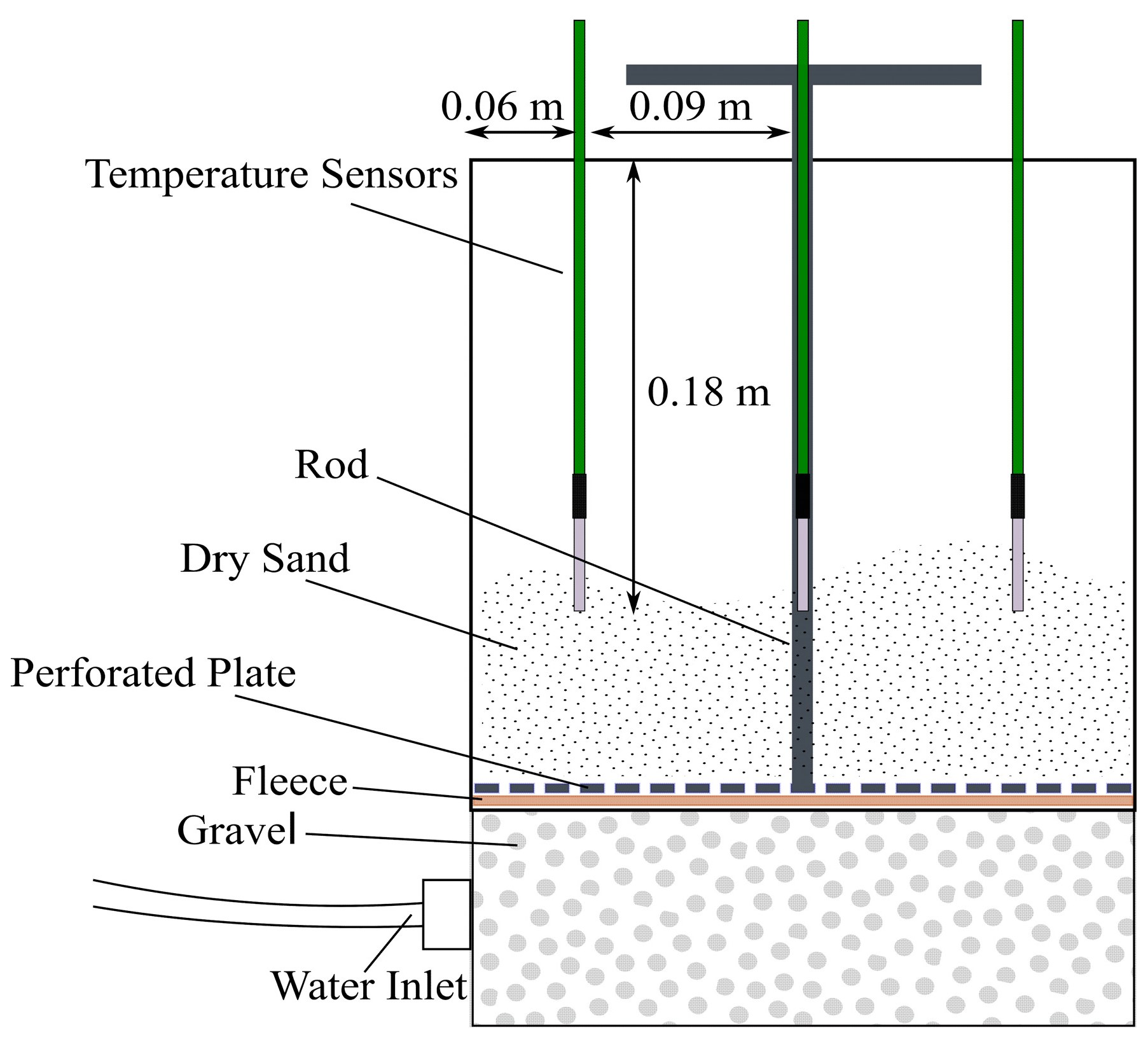
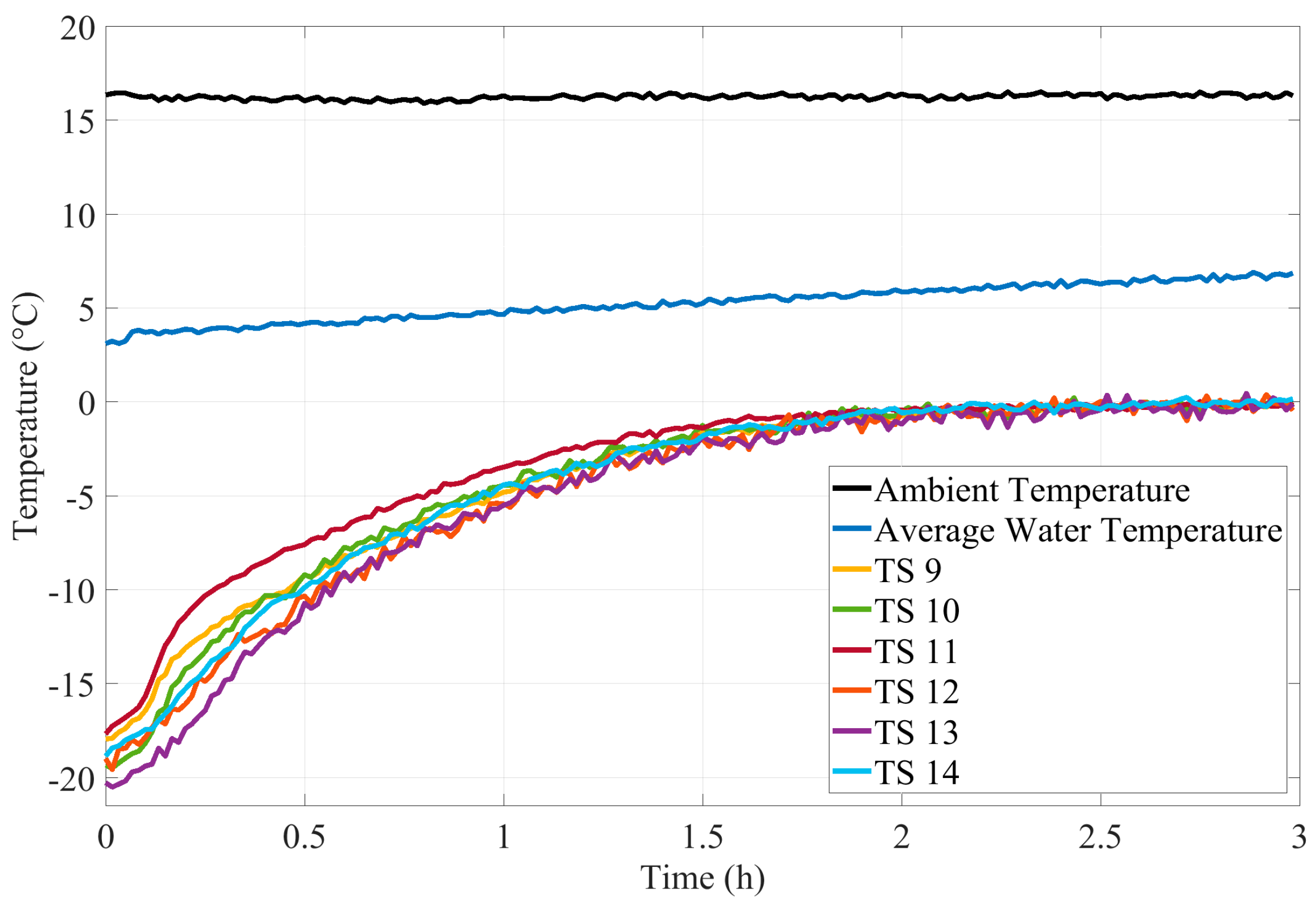
4.1. Development of Permafrost Sample
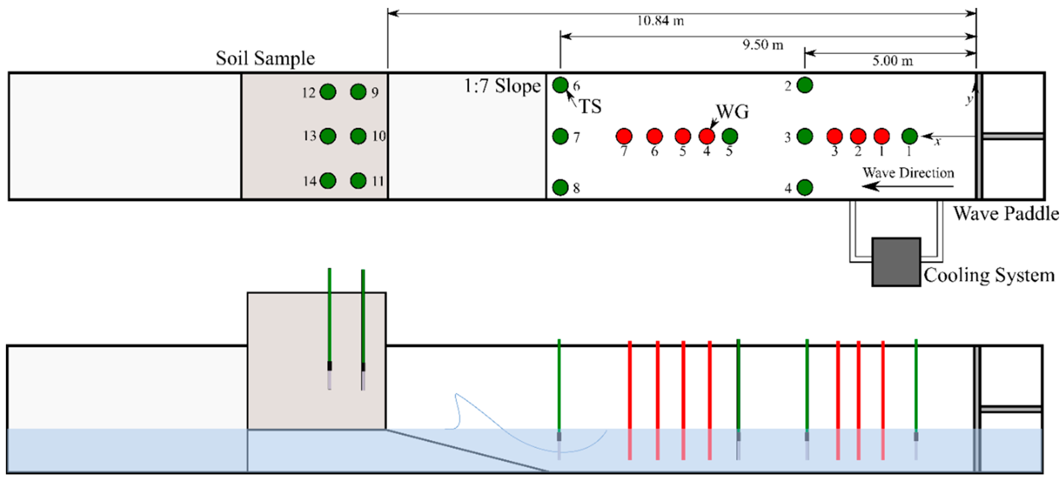
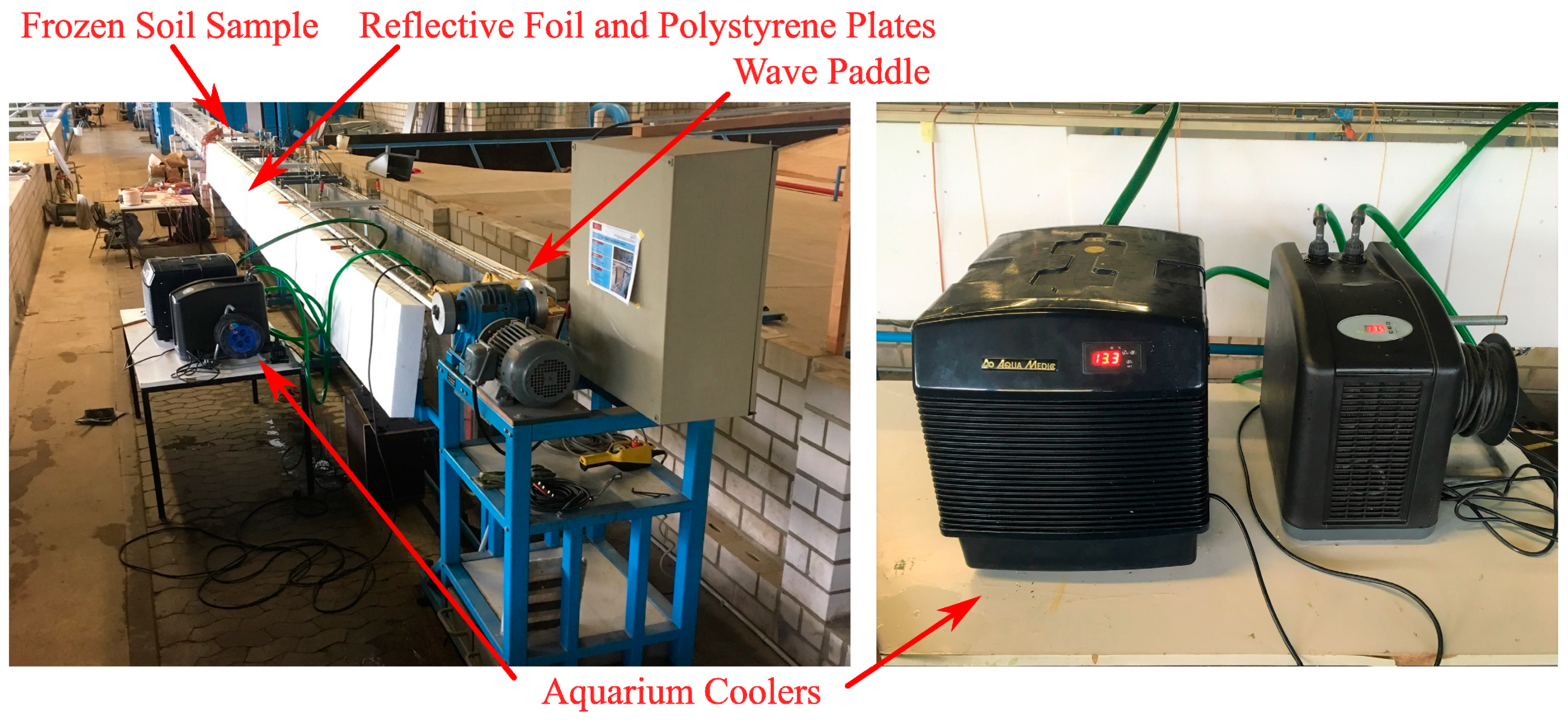
The reproduction of a real permafrost specimen in the laboratory is challenging due to the natural genesis and deposition of sediment as well as challenges in accurately reproducing the macrostructure of the ice [108]. However, as a first approximation, permafrost-like samples were developed for each test as a frozen sand with a fused texture. These activities are interpreted in terms of the overarching framework that was developed and described above; generation zero and one were successfully implemented, with higher generation modelling required to have access to more dedicated laboratory technology, currently unavailable to the authors.
Considering the scaling issues and challenges, sand with a small grain size was the preferable soil for the experiments although, in principle, field samples could also be used; in this study, logistics and availability of field samples drove the choice for simplified samples, though. A small grain size distribution of the sand simplified the method of pluviation and the assessment of the sample reproduction process. With the initial dry sample, sieve analysis was performed to estimate the grain size distribution ( d 50 = 0.0014 m, coefficient of uniformity ( C U ) = 2.25). The mean bulk density ( ρ s = 1508 kg/m3) and void ratio ( n = 0.432) of the sample were determined using the DIN 18126 protocol [109]. The density and the resulting void ration arose from the process of pluviation. The soil sample (0.30 × 0.30 × 0.30 m) was placed in an installation box (to be used for transfer of the specimen from the freeze cabinet to the flume) with a gravel layer at its bottom to allow for an even flow of fluid into the soil specimen from beneath. A perforated metal plate with a threaded rod in the vertical axis of the specimen was installed as a device for lifting the specimen with a crane into the flume. The schematic layout of the installation box is shown in Figure 5. The soil was as evenly as possible placed into the box. In total, six temperature sensors were installed in the sand sample in a regular grid at a depth of 0.18 m (measured from the top of the specimen). Water was injected into the sample through a tube connected to the bottom of the box until the sample was completely saturated. The box was then placed into a freeze cabinet at a temperature of −21.5 °C until the sample had reached equilibrium with the ambient air temperature. The freezing process took about 72 h. Next, the box was transported to the flume where it was installed to be used in the following experiments.

4.2. Wave Tests

The experiments were performed in a 2D wave flume, sketched in Figure 6, at the Leichtweiß-Institute for Hydraulic Engineering and Water Resources (TU Braunschweig, Germany). The experimental setup used a right-handed coordinate system with the origin at the centre of the wave paddle when it was maximally extended towards the soil specimen. The topography of the flume consisted of a flat bottom for the first 9.42 m followed by a 1:7 slope for 1.42 m leading up to the frozen soil sample. The wave analysis was performed by analyzing seven (7) wave gauges (WG—AWP-24-3, Akamina Technologies) placed at x = 3.76, 4.00, 4.35, 6.00, 3.24, 6.59, and 7.00 m.
Temperature sensors (TS—PT-100, SURAN Industrieelektronik, Horb am Neckar, Germany) were placed in the water at two cross-sections ( x = 5.00 m and 9.50 m) and in the longitudinal axis ( x = 2.50 and 7.50 m). The cross sections aimed to investigate any potential cross-flow temperature gradients.
To limit the temperature gradient between the fluid and the soil sample, a cooling system circulating cold water was connected to the flume. Figure 7 shows the equipment and setup used in the experiments conducted for reducing the heat amount of the water inside the wave flume. The two aquarium coolers (1x Aqua Medic Titan 2000, 1x Arcadia AT250, Ritterhude, Germany) achieved a minimum temperature of 9.5 °C in a serial connection. The cooling system was turned off before the wave tests were started. The ambient temperature of the air was approximately 16 °C. A reflecting foil and polystyrene plates (Figure 7) with a thickness of 0.10 m were placed around the outside of the flume to limit temperature changes of the fluid.

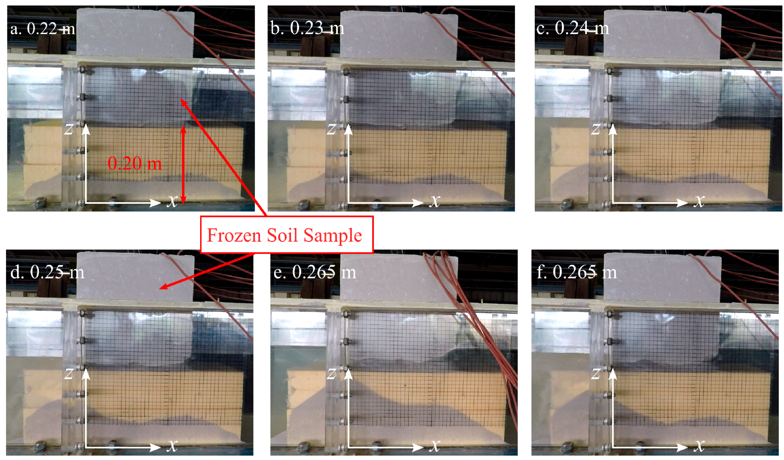
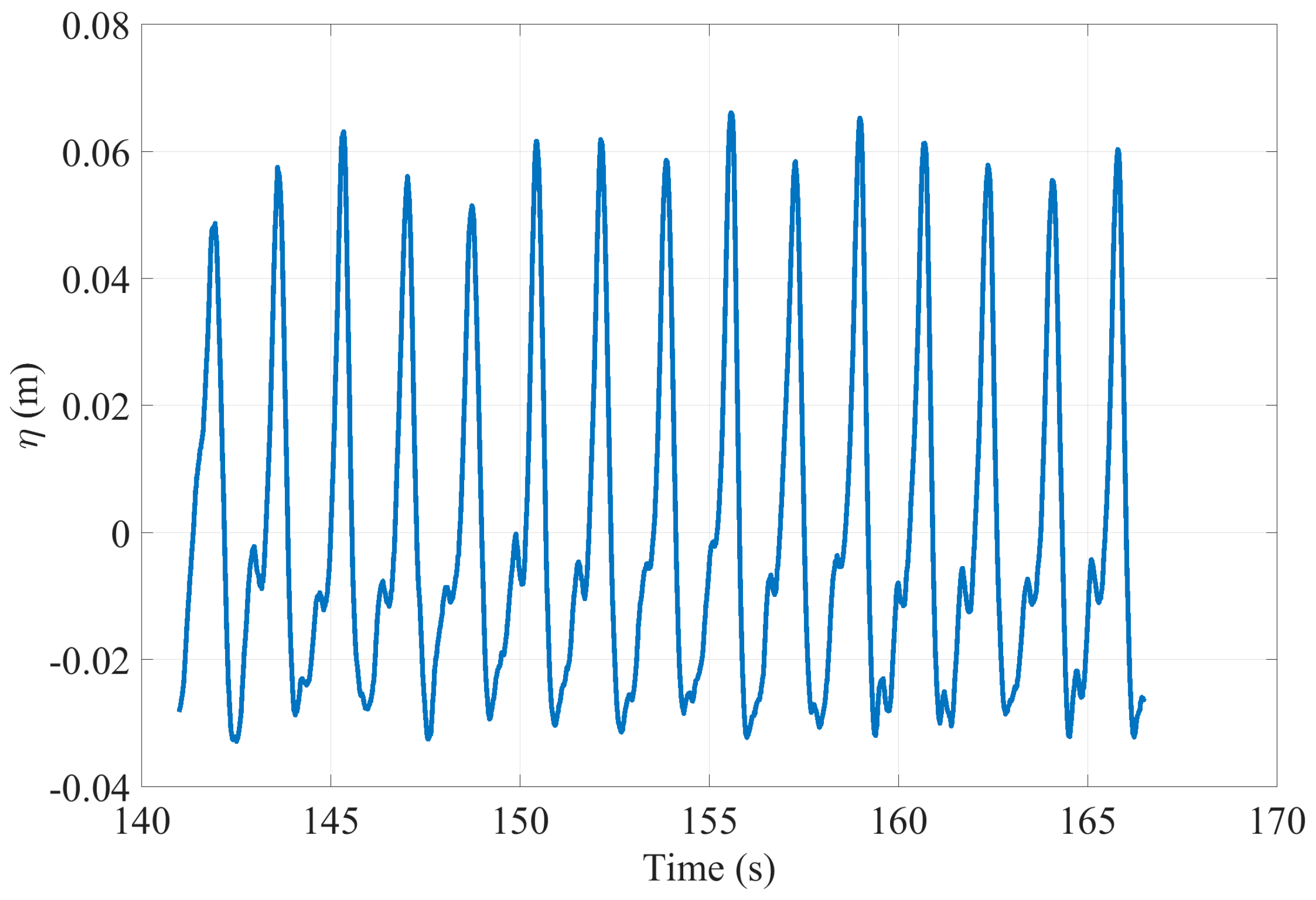
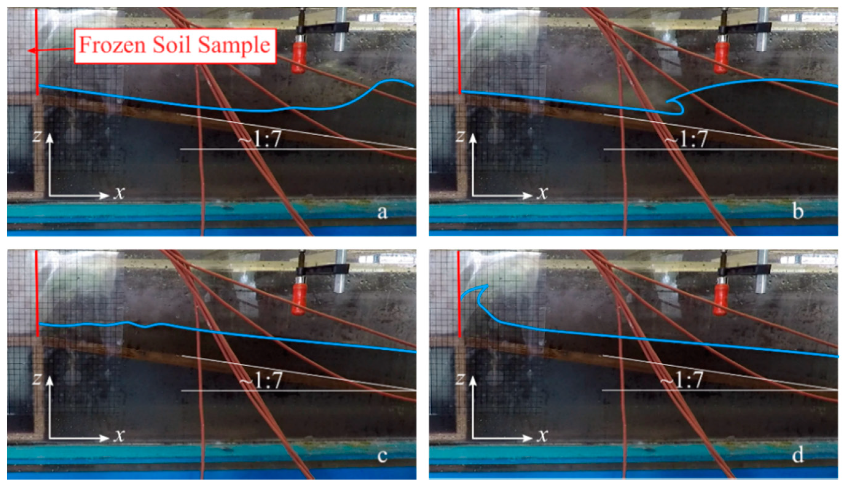
4.3. Experimental Program

Three experiments were performed to analyze the thermal and mechanical contributions to the erosion of permafrost coastlines. Table 2 comprises the detailed information about each experiment. The first experiment examined how the frozen soil specimen interacted with the ambient air temperature in the laboratory. The second experiment examined the interaction between the frozen soil, ambient air, and the water, with an initial deep-water depth of 0.20 m. The final experiment examined both the thermal and mechanical interactions using a regular wave train with H = 0.085 m, T = 1.7 s, and N = 420, being the total number of waves propagated towards the soil specimen. The respective results of the first and second test served as a base for the final experiment to identify limitations and improve the experimental preparation, setup, and timing.

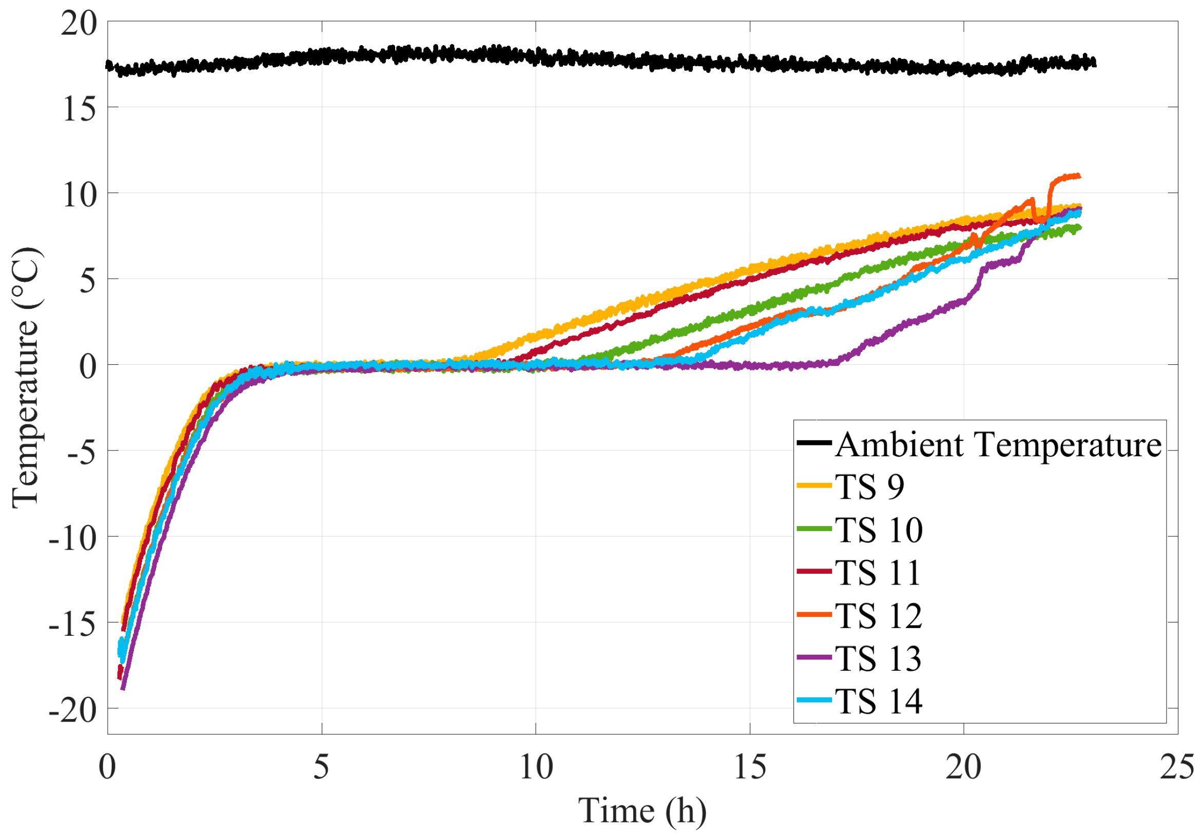
5. Results and Discussion

The identification of the interaction between the ambient temperature and the frozen soil sample was necessary to examine the maximum duration of further experiments. Without being exposed to water, the specimen was lifted into the flume where the sample defrosted from −21.5 to 0 °C within 3 to 4 h, as shown in Figure 8, where recordings of the temperature sensors embedded in the soil specimen are plotted. The thawing front developed from the edge of the specimen to the center. The temperature profile also shows the duration of the phase transformation from ice to water that was already observed during the freezing process. As permafrost is defined as permanently below 0 °C, the influence of the ambient temperature has to be considered in cases where temperature control is not possible.
In order to examine the interaction between the frozen soil, ambient air, and the water, the frozen sample was positioned on the polystyrene plates in the flume which was filled with previously cooled water (9.5 °C) to a deep-water level of 0.20 m, at the same height as the bottom edge of the specimen. Raising the water level stepwise, the soil thawed immediately in contact with the water and was washed out by those small currents that occurred (Figure 9) due to the balancing of the water level along the walls of the flume. As a result, the experiment was mainly determined by the water temperature. The temperature sensors inside the specimen did not exhibit a thermal impact of the water in comparison with the temperature profile of the first test as the sensors only record thermal variation in the surrounding medium. However, sensor TS 9 showed a slightly stronger increase of the temperature at the beginning.
In preparation for the wave tests, attempts were made to reduce the water temperature below 9.5 °C. Using molten ice (about 100 kg of ice cubes added to the flume water), the water temperature decreased to 2–3 °C (water level 0.20 m). Furthermore, the polystyrene plates were replaced by a wooden sub-construction due to issue related to the buoyancy. The regular wave train revealed the development of a thermoerosional niche within the first 10 to 12 min. The wave profile (WG7) of the measured wave heights within the first minutes of Exp. 3 shows the nonlinear characteristic of the waves and the superposition of incident and reflected waves (Figure 10).
The niche developed on the whole length of the specimen (0.30 m) with a height of 0.03 m, yet no block failure occurred. Due to the threaded rod used to transport the sample, the failure mechanism was impeded as the rod provided structural integrity to the sample. Figure 11 shows the development of the thermoerosional niche from a side and front view. The red line in the side view illustrates the shape of the niche as the high turbidity of the water due to sediment wash out impedes a precise measurement. However, the shape of the niche was rather irregular as the sediment close to the flume wall eroded faster than in the middle of the specimen. The grid attached on the side allows a rough assessment of the erosion rate. Within the first 12 min of the test, the waves ( N = 420) caused an erosion of approximately 2700 cm3 of sediment.
Wave breaking was characterized by a plunging breaker, which is typical for steep slopes and a higher wave steepness. The process of wave breaking is shown in Figure 12.
When the niche was fully developed, wave transmission occurred. At this point, a barrier was installed behind the sample in order to observe any possible continuing erosion due to wave reflection at the end of the niche. Wave transmission was attributed to the finite length of the frozen sand sample which does not exist on permafrost coastlines. Therefore, the installation of the barrier was an attempt to reduce this effect on the wave profile. After installing the barrier, the wave reflection caused a backward development of the niche’s height so that the total height summed up to 0.04 m. The erosion process ended after approximately 50 min. For evaluating purposes an isolated consideration of the erosion rate was performed for two timeframes (a) 0 to 12 min and (b) 12 to 50 min. The temperature profile of this test (Figure 13) shows a slightly stronger increase of temperature at the sensors TS 9, TS 10 and TS 11.
This is at the beginning of the test, which can be traced to the thermal impact of the wave run up. However, a significant influence of the water temperature can not be concluded from the temperature profile, as the continuous thawing of the sample was due to the ambient temperature. The ambient air temperature was one of the limiting factors in the experiments and could not be adequately controlled in this setup. Although insulation was installed previously around the flume, there was still continuous heating of the water throughout the tests, in this test reaching approximately 2 °C/h. Despite this observation, there was apparently no development of a significant temperature gradient in the cross-sectional direction. Similarly, there was no obvious temperature gradient developed within the soil sample itself.

6. Conclusions

Erosion along coastlines is a worldwide phenomenon but, in the face of climate change, one of the most concerning changes has centered around the rapid coastal retreat of permafrost coastlines. Analytical and observational investigations on the recession of permafrost coastline provide valuable information about local ecosystems and changes of the coasts. Processes, such as the thermoerosional block failure, and shoreface development, have been modelled successfully and data from field observations prove existing analytical models. However, process-based models with a predictive character and detailed descriptions of the interaction between permafrost and the coastal environment are not yet available. Contrary to observational studies, explanatory variables can be controlled in physical models, although it generally requires a reductionist approach. The authors presented a framework of model generations comprising six stages of complexity in physical modelling. In a first experimental series, a zeroth- and first-generational model revealed aspects that need to be addressed for future modelling of permafrost erosion in coastal environments and allow for an early evaluation of what seems the start of experimental permafrost analysis in coastal environments, now for the first time embedded in an overarching framework of experimental model generations. Summarizing these early findings, the most challenging aspect related to the laboratory setup include the reconstitution of a homogenous soil specimen and the temperature control. Current difficulties are rather logistic challenges so that relations between wave height/length/period and the erosion rate can not be drawn precisely at this point. Furthermore, scaling issues remain unclear and difficult to define as comparable scale series data have not been developed. However, despite these outlined challenges, the development of the thermoerosional niche was successfully observed and this experimental setup revealed the feasibility of a laboratory investigation of coastal permafrost erosion.
The generational model presented here provides a path forward to realizing coastal engineering experimental facilities capable of modelling permafrost and ice-rich environments. Future experimental work could focus on an improved reconstitution of a frozen soil sample and a setup within a cooled environment, such as a cold room. Comparable scale series data need to be developed to define scaling issues and the interaction of hydrodynamic and thermodynamic processes. As climate change continues to make the Arctic more accessible, modelling these environments will be important for a wide-range of sectors, including transportation, energy, and mining. Developing methodologies and process-based approaches to estimating permafrost erosion will not only allow the capturing of uncertainties in design conditions but will also allow for the testing of new solutions, which can improve structures built in these environments.

Author Contributions

Concept development, J.S. and N.G.; Conducting the laboratory tests, S.K.; Developing the methodology and carrying out the analysis of results, S.K., R.G., J.S. and N.G.; writing—original draft preparation, J.S.; writing—amending, review and editing, S.K., R.G., J.S. and N.G.; supervision, R.G. and N.G. All authors have read and agreed to the published version of the manuscript.

Funding

This research received no external funding. The authors gratefully acknowledge support by the German Research Foundation and the Open Access Publication Funds of the Technische Universität Braunschweig.

Acknowledgments

The authors gratefully thank Meerwasseraquaristik Dirk Haase for providing two aquarium coolers as well as the Institute for Geomechanics and Geotechnics for providing the equipment for the experimental temperature control. The authors also thank the anonymous reviewers for their comments and suggestions to improve an earlier version of the manuscript.

Conflicts of Interest

The authors declare no conflict of interest.

References

  1. Cai, L.; Alexeev, V.A.; Arp, C.D.; Jones, B.M.; Romanovsky, V.E. Modelling the impacts of projected sea ice decline on the low atmosphere and near-surface permafrost on the North Slope of Alaska. Int. J. Climatol. 2018, 38, 5491–5504. [Google Scholar] [CrossRef]
  2. Coch, C.; Lamoureux, S.F.; Knoblauch, C.; Eischeid, I.; Fritz, M.; Obu, J.; Lantuit, H. Summer rainfall dissolved organic carbon, solute, and sediment fluxes in a small Arctic coastal catchment on Herschel Island (Yukon Territory, Canada). Arct. Sci. 2018, 4, 750–780. [Google Scholar] [CrossRef] [Green Version]
  3. Biskaborn, B.K.; Smith, S.L.; Noetzli, J.; Matthes, H.; Vieira, G.; Streletskiy, D.A.; Schoeneich, P.; Romanovsky, V.E.; Lewkowicz, A.G.; Abramov, A.; et al. Permafrost is warming at a global scale. Nat. Commun. 2019, 10, 264. [Google Scholar] [CrossRef] [PubMed] [Green Version]
  4. Lemmen, D.; James, T.; Warren, F.; Clarke, C. Canada’s Marine Coasts in a Changing Climate; Government of Canada: Ottawa, ON, Canada, 2016.
  5. Macdonald, R.W.; Harner, T.; Fyfe, J. Recent climate change in the Arctic and its impact on contaminant pathways and interpretation of temporal trend data. Sci. Total Environ. 2005, 342, 5–86. [Google Scholar] [CrossRef] [PubMed]
  6. Lantuit, H.; Overduin, P.P.; Couture, N.; Wetterich, S.; Aré, F.; Atkinson, D.; Brown, J.; Cherkashov, G.; Drozdov, D.; Forbes, D.L. The Arctic coastal dynamics database: A new classification scheme and statistics on Arctic permafrost coastlines. Estuaries Coasts 2012, 35, 383–400. [Google Scholar] [CrossRef] [Green Version]
  7. Harris, S.; French, H.; Heginbottom, J.; Johnston, G.; Ladanyi, B.; Sego, D.; van Everdingen, R. Glossary of Permafrost and Related Ground-Ice Terms; National Research Council: Ottawa, ON, Canada, 1988; ISBN 0-660-125404. [Google Scholar]
  8. Lantuit, H.; Pollard, W.H. Fifty years of coastal erosion and retrogressive thaw slump activity on Herschel Island, southern Beaufort Sea, Yukon Territory, Canada. Geomorphology 2008, 95, 84–102. [Google Scholar] [CrossRef]
  9. Lantuit, H.; Atkinson, D.; Paul Overduin, P.; Grigoriev, M.; Rachold, V.; Grosse, G.; Hubberten, H.-W. Coastal erosion dynamics on the permafrost-dominated Bykovsky Peninsula, North Siberia, 1951–2006. Polar Res. 2011, 30, 7341. [Google Scholar] [CrossRef]
  10. Irrgang, A.M.; Lantuit, H.; Manson, G.K.; Günther, F.; Grosse, G.; Overduin, P.P. Variability in rates of coastal change along the Yukon Coast, 1951 to 2015. J. Geophys. Res. 2018, 123, 779–800. [Google Scholar] [CrossRef] [Green Version]
  11. Lantuit, H.; Overduin, P.P.; Wetterich, S. Recent progress regarding permafrost coasts. Permafr. Periglac. Process. 2013, 24, 120–130. [Google Scholar] [CrossRef]
  12. Jones, B.M.; Arp, C.D.; Jorgenson, M.T.; Hinkel, K.M.; Schmutz, J.A.; Flint, P.L. Increase in the rate and uniformity of coastline erosion in Arctic Alaska. Geophys. Res. Lett. 2009, 36, 1–5. [Google Scholar] [CrossRef]
  13. Cunliffe, A.M.; Tanski, G.; Radosavljevic, B.; Palmer, W.F.; Sachs, T.; Lantuit, H.; Kerby, J.T.; Myers-Smith, I.H. Rapid retreat of permafrost coastline observed with aerial drone photogrammetry. Cryosphere 2019, 13, 1513–1528. [Google Scholar] [CrossRef] [Green Version]
  14. Ford, J.D.; Smit, B. A framework for assessing the vulnerability of communities in the Canadian Arctic to risks associated with climate change. Arctic 2004, 57, 389–400. [Google Scholar] [CrossRef]
  15. Pearce, T.; Smit, B. Vulnerability and adaptation to climate change in the Canadian Arctic. Clim. Vulnerability 2013, 4, 293–303. [Google Scholar] [CrossRef]
  16. Irrgang, A.M.; Lantuit, H.; Gordon, R.R.; Piskor, A.; Manson, G.K. Impacts of past and future coastal changes on the Yukon coast—Threats for cultural sites, infrastructure, and travel routes. Arct. Sci. 2019, 5, 107–126. [Google Scholar] [CrossRef] [Green Version]
  17. Yoon, J.-R.; Kim, Y.-D. Reviews on natural resources in the Arctic: Petroleum, gas, gas hydrates and minerals. Ocean Polar Res. 2001, 23, 51–62. [Google Scholar]
  18. Tolvanen, A.; Eilu, P.; Juutinen, A.; Kangas, K.; Kivinen, M.; Markovaara-Koivisto, M.; Naskali, A.; Salokannel, V.; Tuulentie, S.; Similä, J. Mining in the Arctic environment–A review from ecological, socioeconomic and legal perspectives. J. Environ. Manag. 2019, 233, 832–844. [Google Scholar] [CrossRef]
  19. Lantuit, H.; Rachold, V.; Pollard, W.H.; Steenhuisen, F.; Ødegård, R.; Hubberten, H.-W. Towards a calculation of organic carbon release from erosion of Arctic coasts using non-fractal coastline datasets. Mar. Geol. 2009, 257, 1–10. [Google Scholar] [CrossRef]
  20. Vonk, J.E.; Sánchez-García, L.; van Dongen, B.E.; Alling, V.; Kosmach, D.; Charkin, A.; Semiletov, I.P.; Dudarev, O.V.; Shakhova, N.; Roos, P. Activation of old carbon by erosion of coastal and subsea permafrost in Arctic Siberia. Nature 2012, 489, 137. [Google Scholar] [CrossRef]
  21. Couture, N.J.; Irrgang, A.; Pollard, W.; Lantuit, H.; Fritz, M. Coastal erosion of permafrost soils along the Yukon Coastal plain and fluxes of organic carbon to the Canadian Beaufort Sea. J. Geophys. Res. Biogeosci. 2018, 123, 406–422. [Google Scholar] [CrossRef]
  22. Ramage, J.L.; Irrgang, A.M.; Morgenstern, A.; Lantuit, H. Increasing coastal slump activity impacts the release of sediment and organic carbon into the Arctic Ocean. Biogeosciences 2018, 15, 1483–1495. [Google Scholar] [CrossRef] [Green Version]
  23. Klein, K.P.; Lantuit, H.; Heim, B.; Fell, F.; Doxaran, D.; Irrgang, A.M. Long-term high-resolution sediment and sea surface temperature spatial patterns in Arctic nearshore waters retrieved using 30-year landsat archive imagery. Remote Sens. 2019, 11, 2791. [Google Scholar] [CrossRef] [Green Version]
  24. Outridge, P.M.; Macdonald, R.W.; Wang, F.; Stern, G.A.; Dastoor, A.P. A mass balance inventory of mercury in the Arctic Ocean. Environ. Chem. 2008, 5, 89–111. [Google Scholar] [CrossRef] [Green Version]
  25. Are, F.E. Thermal Abrasion of Seacoasts; Nauka Press: Moscow, Russia, 1988; ISBN 0273-8457. [Google Scholar]
  26. Wobus, C.; Anderson, R.; Overeem, I.; Matell, N.; Clow, G.; Urban, F. Thermal erosion of a permafrost coastline: Improving process-based models using time-lapse photography. Arct. Antarct. Alp. Res. 2011, 43, 474–484. [Google Scholar] [CrossRef]
  27. Manson, G.K.; Solomon, S.M.; Forbes, D.L.; Atkinson, D.E.; Craymer, M. Spatial variability of factors influencing coastal change in the western Canadian Arctic. Geo-Mar. Lett. 2005, 25, 138–145. [Google Scholar] [CrossRef]
  28. Overeem, I.; Anderson, R.S.; Wobus, C.W.; Clow, G.D.; Urban, F.E.; Matell, N. Sea ice loss enhances wave action at the Arctic coast. Geophys. Res. Lett. 2011, 38, 1–6. [Google Scholar] [CrossRef]
  29. Kobayashi, N.; Vidrine, J.C.; Nairn, R.B.; Soloman, S.M. Erosion of frozen cliffs due to storm surge on Beaufort Sea Coast. J. Coast. Res. 1999, 15, 332–344. [Google Scholar]
  30. Lantuit, H.; Pollard, W.H. Temporal stereophotogrammetric analysis of retrogressive thaw slumps on Herschel Island, Yukon Territory. Nat. Hazards Earth Syst. Sci. 2005, 5, 413–423. [Google Scholar] [CrossRef] [Green Version]
  31. Lantuit, H.; Pollard, W.H.; Couture, N.; Fritz, M.; Schirrmeister, L.; Meyer, H.; Hubberten, H.-W. Modern and late Holocene retrogressive thaw slump activity on the Yukon coastal plain and Herschel Island, Yukon Territory, Canada. Permafr. Periglac. Process. 2012, 23, 39–51. [Google Scholar] [CrossRef]
  32. Hoque, M.A.; Pollard, W.H. Stability of permafrost dominated coastal cliffs in the Arctic. Polar Sci. 2016, 10, 79–88. [Google Scholar] [CrossRef]
  33. Guégan, E.B.M.; Christiansen, H.H. Seasonal Arctic coastal bluff dynamics in Adventfjorden, Svalbard. Permafr. Periglac. Process. 2017, 28, 18–31. [Google Scholar] [CrossRef]
  34. Hughes, S.A. Physical Models and Laboratory Techniques in Coast. Eng.; World Scientific: Singapore, 1993; ISBN 981021541X. [Google Scholar]
  35. Tsytovich, N. The Mechanics of Frozen Ground (Translated); Scripta Book Company: Lansing, MI, USA, 1975. [Google Scholar]
  36. Osterkamp, T.; Burn, C. Permafrost, 1st ed.; Academic Press: Cambridge, MA, USA, 2003. [Google Scholar]
  37. Cannone, N.; Wagner, D.; Hubberten, H.W.; Guglielmin, M. Biotic and abiotic factors influencing soil properties across a latitudinal gradient in Victoria Land, Antarctica. Geoderma 2008, 144, 50–65. [Google Scholar] [CrossRef] [Green Version]
  38. Zhang, T.; Osterkamp, T.E.; Stamnes, K. Effects of climate on the active layer and permafrost on the north slope of Alaska, USA. Permafrost Periglac. Process. 1997, 8, 45–67. [Google Scholar] [CrossRef]
  39. Deprez, M.; de Kock, T.; de Schutter, G.; Cnudde, V. A review on freeze-thaw action and weathering of rocks. Earth-Sci. Rev. 2020, 203, 103143. [Google Scholar] [CrossRef]
  40. Harry, D.G.; Gozdzik, J.S. Ice wedges: Growth, thaw transformation, and palaeoenvironmental significance. J. Quat. Sci. 1988, 3, 39–55. [Google Scholar] [CrossRef]
  41. Yang, Z.; Still, B.; Ge, X. Mechanical properties of seasonally frozen and permafrost soils at high strain rate. Cold Reg. Sci. Technol. 2015, 113, 12–19. [Google Scholar] [CrossRef]
  42. Callaghan, D.P.; Nielsen, P.; Short, A.; Ranasinghe, R. Statistical simulation of wave climate and extreme beach erosion. Coast. Eng. 2008, 55, 375–390. [Google Scholar] [CrossRef]
  43. Larson, M.; Erikson, L.; Hanson, H. An analytical model to predict dune erosion due to wave impact. Coast. Eng. 2004, 51, 675–696. [Google Scholar] [CrossRef]
  44. McCall, R.T.; van Thiel de Vries, J.S.M.; Plant, N.G.; van Dongeren, A.R.; Roelvink, J.A.; Thompson, D.M.; Reniers, A.J.H.M. Two-dimensional time dependent hurricane overwash and erosion modeling at Santa Rosa Island. Coast. Eng. 2010, 57, 668–683. [Google Scholar] [CrossRef]
  45. Roelvink, D.; Reniers, A.; van Dongeren, A.; van Thiel de Vries, J.; McCall, R.; Lescinski, J. Modelling storm impacts on beaches, dunes and barrier islands. Coast. Eng. 2009, 56, 1133–1152. [Google Scholar] [CrossRef]
  46. van Thiel de Vries, J.S.M.; van Gent, M.R.A.; Walstra, D.J.R.; Reniers, A.J.H.M. Analysis of dune erosion processes in large-scale flume experiments. Coast. Eng. 2008, 55, 1028–1040. [Google Scholar] [CrossRef]
  47. Holthuijsen, L.H. Waves in Oceanic and Coastal Waters; Cambridge University Press: Cambridge, MA, USA, 2007; ISBN 9780511618536. [Google Scholar]
  48. Madsen, O.S.; Grant, W.D. Quantitative description of sediment transport by waves. Coast. Eng. 1976, 15, 1092–1112. [Google Scholar] [CrossRef] [Green Version]
  49. Hanley, M.E.; Hoggart, S.P.G.; Simmonds, D.J.; Bichot, A.; Colangelo, M.A.; Bozzeda, F.; Heurtefeux, H.; Ondiviela, B.; Ostrowski, R.; Recio, M.; et al. Shifting sands? Coastal protection by sand banks, beaches and dunes. Coast. Eng. 2014, 87, 136–146. [Google Scholar] [CrossRef]
  50. Bruun, P. Coastal Erosion and the Development of Beach Profiles; Technical Memorandum No. 44, U.S. Beach Erosion Board; US Army Engineer Research and Development Center (ERDC): Vicksburg, MS, USA, 1954. [Google Scholar]
  51. Trenhaile, A.S. Modeling the erosion of cohesive clay coasts. Coast. Eng. 2009, 56, 59–72. [Google Scholar] [CrossRef]
  52. Ogorodov, S.A.; Baranskaya, A.V.; Belova, N.G.; Kamalov, A.M.; Kuznetsov, D.E.; Overduin, P.P.; Shabanova, N.N.; Vergun, A.P. Coastal dynamics of the Pechora and Kara Seas under changing climatic conditions and human disturbances. Geogr. Environ. Sustain. 2016, 9, 53–73. [Google Scholar] [CrossRef]
  53. Hoque, M.A.; Pollard, W.H. Arctic coastal retreat through block failure. Can. Geotech. J. 2009, 46, 1103–1115. [Google Scholar] [CrossRef]
  54. Forbes, D.L.; Taylor, R.B. Ice in the shore zone and the geomorphology of cold coasts. Prog. Phys. Geogr. 1994, 18, 59–89. [Google Scholar] [CrossRef]
  55. Kovacs, A.; Sodhi, D.S. Ice pile-up and ride-up on arctic and subarctic beaches. Coast. Eng. 1981, 5, 247–273. [Google Scholar] [CrossRef]
  56. Ettema, R. Review of alluvial-channel responses to river ice. J. Cold Reg. Eng. 2002, 16, 191–217. [Google Scholar] [CrossRef]
  57. Ettema, R.; Baker, J.L.; Howlett, G.; Hudson, B. Ice-floe impact with a rubble-mound causeway at the port of nome, alaska. J. Cold Reg. Eng. 2019, 33, 5019001. [Google Scholar] [CrossRef]
  58. Ettema, R.; Zabilansky, L. Ice influences on channel stability: Insights from missouri’s fort peck reach. J. Hydraul. Eng. 2004, 130, 279–292. [Google Scholar] [CrossRef]
  59. Balmer, R.T. Modern Engineering Thermodynamics-Textbook with Tables Booklet; Academic Press: Cambridge, MA, USA, 2011; ISBN 0123850738. [Google Scholar]
  60. Costard, F.; Dupeyrat, L.; Gautier, E.; Carey-Gailhardis, E. Fluvial thermal erosion investigations along a rapidly eroding river bank: Application to the Lena River (central Siberia). Earth Surf. Process. Landf. 2003, 28, 1349–1359. [Google Scholar] [CrossRef]
  61. Veuille, S.; Fortier, D.; Verpaelst, M.; Grandmont, K.; Charbonneau, S. Heat advection in the active layer of permafrost: Physical modelling to quantify the impact of subsurface flow on soil thawing. In Proceedings of the 7th Canadian Conference on Permafrost and 68th Canadian Conference on Geotechnic, Quebec City, QC, Canada, 21–23 September 2015 ; pp. 20–23. [Google Scholar]
  62. Manson, G.K.; Solomon, S.M. Past and future forcing of beaufort sea coastal change. Atmosphere-Ocean 2007, 45, 107–122. [Google Scholar] [CrossRef]
  63. Budetta, P.; Galietta, G.; Santo, A. A methodology for the study of the relation between coastal cliff erosion and the mechanical strength of soils and rock masses. Eng. Geol. 2000, 56, 243–256. [Google Scholar] [CrossRef]
  64. Dean, R.G. Physical modelling of littoral processes. Phys. Model. Coast. Eng. 1985, 1, 119–139. [Google Scholar]
  65. Are, F.; Reimnitz, E. The a and m coefficients in the Bruun/Dean equilibrium profile equation seen from the Arctic. J. Coast. Res. 2008, 2, 243–249. [Google Scholar] [CrossRef]
  66. Kobayashi, N. Formation of thermoerosional niches into frozen bluffs due to storm surges on the Beaufort Sea coast. J. Geophys. Res. 1985, 90, 11983–11988. [Google Scholar] [CrossRef]
  67. Pogojeva, M.; Yakushev, E.; Ilinskaya, A.; Polukhin, A.; Braaten, H.-F.; Kristiansen, T. Experimental study of the influence of thawing permafrost on the chemical properties of sea water. Russ. J. Earth Sci. 2018, 18. [Google Scholar] [CrossRef] [Green Version]
  68. Stettner, S.; Beamish, A.; Bartsch, A.; Heim, B.; Grosse, G.; Roth, A.; Lantuit, H. Monitoring inter- and intra-seasonal dynamics of rapidly degrading ice-rich permafrost riverbanks in the Lena delta with TerraSAR-X time series. Remote Sens. 2018, 10, 51. [Google Scholar] [CrossRef] [Green Version]
  69. Obu, J.; Lantuit, H.; Grosse, G.; Günther, F.; Sachs, T.; Helm, V.; Fritz, M. Coastal erosion and mass wasting along the Canadian Beaufort Sea based on annual airborne LiDAR elevation data. Geomorphology 2017, 293, 331–346. [Google Scholar] [CrossRef] [Green Version]
  70. Holthuijsen, L.H.; Booij, N.; Herbers, T.H.C. A prediction model for stationary, short-crested waves in shallow water with ambient currents. Coast. Eng. 1989, 13, 23–54. [Google Scholar] [CrossRef]
  71. Afzal, M.S.; Bihs, H.; Kamath, A.; Arntsen, Ø.A. Three-dimensional numerical modeling of pier scour under current and waves using level-set method. J. Offshore Mech. Arct. Eng. 2015, 137. [Google Scholar] [CrossRef]
  72. Ahmad, N.; Bihs, H.; Myrhaug, D.; Kamath, A.; Arntsen, Ø.A. Numerical modeling of breaking wave induced seawall scour. Coast. Eng. 2019, 150, 108–120. [Google Scholar] [CrossRef]
  73. Sumer, B.M.; Whitehouse, R.J.S.; Tørum, A. Scour around coastal structures: A summary of recent research. Coast. Eng. 2001, 44, 153–190. [Google Scholar] [CrossRef]
  74. Hall, J.W.; Meadowcroft, I.C.; Lee, E.M.; van Gelder, P.H.A.J.M. Stochastic simulation of episodic soft coastal cliff recession. Coast. Eng. 2002, 46, 159–174. [Google Scholar] [CrossRef]
  75. Russell-Head, D.S. The melting of free-drifting icebergs. Ann. Glaciol. 1980, 1, 119–122. [Google Scholar] [CrossRef] [Green Version]
  76. White, F.M.; Spaulding, M.L.; Gominho, L. Theoretical Estimates of the Various Mechanisms Involved in Iceberg Deterioration in the Open Ocean Environment; Rhode Island University: Kingston, RI, USA, 1980. [Google Scholar]
  77. Barnhart, K.R.; Anderson, R.S.; Overeem, I.; Wobus, C.; Clow, G.D.; Urban, F.E. Modeling erosion of ice-rich permafrost bluffs along the Alaskan Beaufort Sea coast. J. Geophys. Res. 2014, 119, 1155–1179. [Google Scholar] [CrossRef]
  78. Ahmad, N.; Bihs, H.; Chella, M.A.; Kamath, A.; Arntsen, Ø.A. CFD modeling of arctic coastal erosion due to breaking waves. ISOPE-19-29-1-033 2019, 29, 33–41. [Google Scholar] [CrossRef] [Green Version]
  79. Kobayashi, N.; Aktan, D. Thermoerosion of frozen sediment under wave action. J. Waterw. Port Coast. Ocean Eng. 1986, 112, 140–158. [Google Scholar] [CrossRef]
  80. Dupeyrat, L.; Costard, F.; Randriamazaoro, R.; Gailhardis, E.; Gautier, E.; Fedorov, A. Effects of ice content on the thermal erosion of permafrost: Implications for coastal and fluvial erosion. Permafr. Periglac. Process. 2011, 22, 179–187. [Google Scholar] [CrossRef]
  81. Overduin, P.P.; Schneider von Deimling, T.; Miesner, F.; Grigoriev, M.N.; Ruppel, C.; Vasiliev, A.; Lantuit, H.; Juhls, B.; Westermann, S. Submarine permafrost map in the arctic modeled using 1-D transient heat flux (SuPerMAP). J. Geophys. Res. 2019, 124, 3490–3507. [Google Scholar] [CrossRef] [Green Version]
  82. MacMahan, J.; Thornton, E.; Koscinski, J.; Wang, Q. Field observations and modeling of surfzone sensible heat flux. J. Appl. Meteorol. Climatol. 2018, 57, 1371–1383. [Google Scholar] [CrossRef]
  83. Sinnett, G.; Feddersen, F. The competing effects of breaking waves on surfzone heat fluxes: Albedo versus wave heating. J. Geophys. Res. 2018, 123, 7172–7184. [Google Scholar] [CrossRef]
  84. Heller, V. Scale effects in physical hydraulic engineering models. J. Hydraul. Res. 2011, 49, 293–306. [Google Scholar] [CrossRef]
  85. Kamphuis, J.W. Physical modelling. In Herbich, Herbich (Hg.) 1991–Handbook of Coastal and Ocean Engineering; Gulf professional Publishing: Houston, TX, USA, 1992. [Google Scholar]
  86. Davies, M.C.R.; Hamza, O.; Harris, C. Physical modelling of permafrost warming in rock slopes. In Proceedings of the 8th International Conference on Permafrost, Lisse, The Netherlands, 21–25 July 2003; pp. 169–173. [Google Scholar]
  87. Dong, Y.; Lu, N.; McCartney, J.S. Scaling shear modulus from small to finite strain for unsaturated soils. J. Geotech. Geoenviron. Eng. 2018, 144, 4017110. [Google Scholar] [CrossRef] [Green Version]
  88. Timco, G.W.; Weeks, W.F. A review of the engineering properties of sea ice. Cold Reg. Sci. Technol. 2010, 60, 107–129. [Google Scholar] [CrossRef]
  89. Hopkins, M.A. Onshore ice pile-up: A comparison between experiments and simulations. Cold Reg. Sci. Technol. 1997, 26, 205–214. [Google Scholar] [CrossRef]
  90. Zhou, L.; Riska, K.; von Bock und Polach, R.; Moan, T.; Su, B. Experiments on level ice loading on an icebreaking tanker with different ice drift angles. Cold Reg. Sci. Technol. 2013, 85, 79–93. [Google Scholar] [CrossRef]
  91. Hirdaris, S.E.; Bai, W.; Dessi, D.; Ergin, A.; Gu, X.; Hermundstad, O.A.; Huijsmans, R.; Iijima, K.; Nielsen, U.D.; Parunov, J. Loads for use in the design of ships and offshore structures. Ocean Eng. 2014, 78, 131–174. [Google Scholar] [CrossRef]
  92. Gao, P.; Le Person, S.; Favre-Marinet, M. Scale effects on hydrodynamics and heat transfer in two-dimensional mini and microchannels. Int. J. Therm. Sci. 2002, 41, 1017–1027. [Google Scholar] [CrossRef] [Green Version]
  93. Incropera, F.P.; Lavine, A.S.; Bergman, T.L.; DeWitt, D.P. Fundamentals of Heat and Mass Transfer; Wiley: Hoboken, NJ, USA, 2007; ISBN 0471457280. [Google Scholar]
  94. Rapp, B.E. Microfluidics. Modeling, Mechanics, and Mathematics; William Andrew: Kidlington, UK, 2017; ISBN 9781455731411. [Google Scholar]
  95. Black, R.F. Permafrost: A review. Geol. Soc. Am. Bull. 1954, 65, 839–856. [Google Scholar] [CrossRef]
  96. Dean, R.G.; Dalrymple, R.A. Water Wave Mechanics for Engineers and Scientists; World Scientific Publishing Company: Singapore, 1991; ISBN 9814365696. [Google Scholar]
  97. Schäffer, H.A.; Klopman, G. Review of multidirectional active wave absorption methods. J. Waterw. Port Coast. Ocean Eng. 2000, 126, 88–97. [Google Scholar] [CrossRef]
  98. Spinneken, J.; Swan, C. The operation of a 3D wave basin in force control. Ocean Eng. 2012, 55, 88–100. [Google Scholar] [CrossRef] [Green Version]
  99. Mathisen, P.P.; Madsen, O.S. Waves and currents over a fixed rippled bed: 2. Bottom and apparent roughness experienced by currents in the presence of waves. J. Geophys. Res. 1996, 101, 16543–16550. [Google Scholar] [CrossRef]
  100. Welzel, M.; Schendel, A.; Hildebrandt, A.; Schlurmann, T. Scour development around a jacket structure in combined waves and current conditions compared to monopile foundations. Coast. Eng. 2019, 152, 103515. [Google Scholar] [CrossRef]
  101. Font, M.; Lagarde, J.-L.; Amorese, D.; Coutard, J.-P.; Dubois, A.; Guillemet, G.; Ozouf, J.-C.; Vedie, E. Physical modelling of fault scarp degradation under freeze–thaw cycles. Earth Surface Process. Landf. 2006, 31, 1731–1745. [Google Scholar] [CrossRef]
  102. Vedie, E.; Lagarde, J.-L.; Font, M. Physical modelling of rainfall-and snowmelt-induced erosion of stony slope underlain by permafrost. E Earth Surface Process. Landf. 2011, 36, 395–407. [Google Scholar] [CrossRef]
  103. Védie, E.; Costard, F.; Font, M.; Lagarde, J.L. Laboratory simulations of Martian gullies on sand dunes. Geophys. Res. Lett. 2008, 35. [Google Scholar] [CrossRef]
  104. Rivière, A.; Jost, A.; Gonçalvès, J.; Font, M. Pore water pressure evolution below a freezing front under saturated conditions: Large-scale laboratory experiment and numerical investigation. Cold Regions Sci. Technol. 2019, 158, 76–94. [Google Scholar] [CrossRef]
  105. Thomas, H.R.; Cleall, P.; Li, Y.-C.; Harris, C.; Kern-Luetschg, M. Modelling of cryogenic processes in permafrost and seasonally frozen soils. Geotechnique 2009, 59, 173–184. [Google Scholar] [CrossRef]
  106. Randriamazaoro, R.; Dupeyrat, L.; Costard, F.; Gailhardis, E.C. Fluvial thermal erosion: Heat balance integral method. Earth Surface Process. Landf. 2007, 32, 1828–1840. [Google Scholar] [CrossRef]
  107. Cataño-Lopera, Y.A.; García, M.H. Geometry and migration characteristics of bedforms under waves and currents. Part 1: Sandwave morphodynamics. Coast. Eng. 2006, 53, 767–780. [Google Scholar] [CrossRef]
  108. Song, A.J.; Lever, J.H.; Bates, S.W. Modeling Relevant to Safe Operations of US Navy Vessels in Arctic Conditions: Physical Modeling of Ice Loads; US Army Engineer Research and Development Center (ERDC): Vicksburg, MS, USA, 2016. [Google Scholar]
  109. DIN. Soil, Investigation and Testing—Determination of Density of Non-Cohesive Soils for Maximum and Minimum Compactness; Deutsches Institut für Normung e.V: Berlin, Germany, 1996. [Google Scholar]
Figure 1. Vertical structure of permafrost soils. The red line shows a conceptual temperature profile through the soil.
Water 12 02254 g001
Figure 2. Visualization of erosion mechanism for the development of a thermoerosional niche and subsequent block failure. Photographic illustrations of the block failure process can be found, e.g., [12].
Water 12 02254 g002
Figure 3. Conceptual modelling of the complexity of permafrost coastlines. The center of the figure shows a conceptual drawing on the prototype conditions. The model complexity will be mapped considering the (a) atmospheric temperature, (b) permafrost vertical structure, (c) wave conditions, and (d) temperature profile within the permafrost.
Water 12 02254 g003
Figure 4. Framework design for investigating laboratory-based permafrost coastline erosion. Permafrost 3D-tank, with media/material indicated by circled symbols, and technical process-influencing technologies indicated by diamond-shaped boxes. A—Wave flume, B—Cooled saltwater, C—Frozen soil samples, D—Insulation layer, E—Generation of waves, F—Small-to-medium scale cold room, G—Water temperature control, H—Heat exchanger capabilities placed along flume of basin walls, I—Generation of currents, J—Slope, K—Ice wedge, L—Soil layers, M—Tidal currents.
Water 12 02254 g004
Figure 5. Installation box (screw system) for the modelling of the frozen sand sample depicting permafrost at lowest model generation. When removing the box for installing the specimen in the flume for further testing, the bottom part (gravel and fleece) was also removed, while the perforated plate and threaded rod remained inside the specimen.
Water 12 02254 g005
Figure 6. Wave flume (20.0 × 0.30 × 0.38 m). Wave gauges (WG) are shown as red and temperature sensors (TS) as green circles.
Water 12 02254 g006
Figure 7. Reflecting foil, polystyrene plates and aquarium cooler (serial connection) for cooling the water and reducing heat flow.
Water 12 02254 g007
Figure 8. Time history of the temperature profile of the PT100 sensors in the soil; positions are according to Figure 6.
Water 12 02254 g008
Figure 9. Frozen soil specimen of Exp. 2 in the flume on polystyrene plates exposed to the hydrostatic water level. The initial deep water depth was 0.20 m. The flume was then slowly filled with water. As the frozen specimen thawed immediately in contact with water, the filling was stopped at a water depth of 0.265 m. Small currents due to the filling process led to a wash out of the loose sediment causing high turbidity. Panels (a)–(f) show the filling of the flume stepwise to the water level that is indicated in each panel.
Water 12 02254 g009
Figure 10. Surface elevation time history of the wave gauge WG7 that was used to test a frozen permafrost specimen.
Water 12 02254 g010
Figure 11. Frozen soil specimen in the flume. The specimen was exposed to a regular wave train (for details see Table 2). The red line marks the development of the thermoerosional niche at the start, after 5 and 10 min. The development of the soil specimen’s front side at the same time. Panels (ac) show a side-view of the frozen soil, while panels (df) present a front view, with time instants ‘start’, ‘5 min’, and ’10 min’ subsequently.
Water 12 02254 g011
Figure 12. Wave breaking in front of the frozen soil sample at the beginning of Exp. 3. The waves are running up a 1:7 ramp and break as plunging breakers due to shoaling effects. The blue lines mark the development of the wave crest. Panels (a)–(d) illustrate the time-history of the surface elevation of the water level in front of the frozen soil sample in a side view.
Water 12 02254 g012
Figure 13. Time history of the temperature profile of test Exp. 3, for the embedded temperature sensors as well as for the water and ambient air temperature; positions are according to Figure 6.
Water 12 02254 g013
Table 1. Generational model approach (Generation 0–5) addressing the parameters critical to the process of thermomechanical erosion.
Generation
Parameter Space2D3D
Parameter CategoryParameter012345
Permafrost Soil ModelVertical Structure of Permafrost × ×
Horizontal Structure of Permafrost ×× ×
Soil Grain Size××××××
Water/Ice Content××××××
Organic Content × ×
Temperature Profile ××××
Hydrodynamic Boundary ConditionsWater Level (Tides, Sea Level Rise)××××××
Regular Waves × ×
Irregular Waves ×× ×
Currents ×× ×
Wave Direction ××
Ambient EnvironmentAir Temperature (passive/active)××××××
Cyclical Time Series × ×
Water Properties/ChemistrySalinity × ×
Water Temperature××××××
Sediment Concentration × ×
Table 2. List of experiments and setup details for the program described herein.
ExperimentWater (Yes/No)Water LevelWave Height/PeriodWater Volume
(-)(-)(m)(m)/(s)(L)
Exp. 1No-/--/--/-
Exp. 2Yes0.20–0.265 -/-650–862
Exp. 3Yes0.200.085/1.7650

