Understanding the Ecological Response of Planktic and Benthic Epipelic Algae to Environmental Factors in an Urban Rivers System

1
School of Computer & Software, Nanjing Institute of Industry Technology, Nanjing 210016, China
2
College of Computer and Information, Hohai University, Nanjing 210098, China
3
Key Laboratory of Integrated Regulation and Resource Development on Shallow Lake of Ministry of Education, College of Environment, Hohai University, Nanjing 210098, China
*
Authors to whom correspondence should be addressed.
Water 2020, 12(5), 1311; https://doi.org/10.3390/w12051311
Submission received: 3 March 2020
/
Revised: 7 April 2020
/
Accepted: 10 April 2020
/
Published: 6 May 2020
(This article belongs to the Special Issue The Response of the Plankton Community to Environmental Stress)
Abstract
:Many studies have been concentrated on the distribution of algae in lakes, rivers, and seas, however, few studies have been concerned about their distribution and relation with polluted urban rivers. In this study, the spatio-temporal variation characteristics of water quality and algae community in Nanjing city were investigated with microscopic examination for one year. Results showed that the water pollution in this area was mainly related to high concentration of nitrogen (NH3-N and TN (Total nitrogen). There was a total of 77 species of algae in the studied rivers from June 2016 to May 2017, among which 73 species of planktic algae and 34 species of epipelic algae, in which the abundance and biomass of the latter were 1925 and 904 times that of the former, respectively. The two kinds of algae had different change tendencies which were related to seasons. For planktic algae, the abundance and biomass decreased in this season sequence: summer, spring, autumn, and winter. For epipelic algae, the abundance and biomass were relatively higher in winter. The dominant community of planktic algae was Chlorophyta-Bacillariophyceae-Cyanobacteria type, while that of epipelic algae was Bacillariophyceae—Cyanobacteria type. Most of the present algae were bi-trophic species, and were tightly related to the pollution characteristics of the rivers. The key environmental factors for planktic algae are T, TN, and TP, and those for Epipelic algae are N:P and TN. The relation between the community composition of planktic and epipelic algae and environmental parameters are highly complex, and it is worth carrying out further study to clarify their interaction mechanism.
1. Introduction
Algae are the primary producer of aquatic ecosystem, and play a key role in material cycling and energy transformation processes [1]. The planktic algae can transform inorganic materials into organic materials via solar energy, and the produced organics are then stored by consumers, which ensured the existence and propagation of algal community [2]. After the death of algae, the residue is degraded by microorganisms, then the produced organic debris either settle to the bottom of a water body or are suspended in a water layer. These micro-particles can again be absorbed to the surface of algae and affect their photosynthesis process. Additionally, the increment of soluble and particular organics in a water body provides abundant nutrients for the growth and propagation of heterotrophic algae and zooplankton which can exist in an environment of organic pollution. When the propagation ability of algae exceeds the degradation ability of heterotrophic bacteria, a great amount of organics will remain in the water body, which is the fundamental reason for water quality degradation of urban rivers [3]. On the other hand, the pollution status of urban waters (particularly nutrient pollution) also affects the spatial and temporal distribution and community structure of algae [4,5,6]. Recently, algae have been introduced as a biological index for water quality assessment [7,8,9], and many studies have been concentrated on the distribution characteristics of planktic algae and epipelic algae in lakes, rivers, and seas, and the relationships between algae communities and environmental parameters [10,11,12,13,14,15].
The relationships between planktic and epipelic algae communities and environmental parameters are highly complex and not yet explained by a unified theory. Various studies have been used to analyze these relationships [16,17,18,19,20,21]. For example, Zhao et al. [17] revealed the main environmental parameters influencing phytoplankton distribution in the Qinhuai River were water temperature (T), conductivity (COND), and TN, and the secondary factors were DO, NH4+-N, NO3-N, CODMn, TN/TP ratio, and oxidation–reduction potential. Light and Beardall [13] reported that organic matter may be important in determining the distribution of benthic microalgal biomass. Çelekli et al. [5] indicated T, heavy metals, and nutrient contents were the major variables driving the spatial and temporal occurrence and biochemical contents of filamentous algae species in various water bodies in Turkey. José et al. [22] found that the annual flood was the main driving force for seasonal and spatial variation of benthic algal crops. Gao et al. [4] showed physicochemical variables, including TP, T, and salinity, were the most important factors influencing the variation of phytoplankton community structure. Winter et al. [18] found the changes in the phytoplankton community of Lake Simcoe were related to nutrient load reductions, the invasion of zebra mussels, and increasing water column stability. Naselli-Flores [19] indicated T, conduction, and storage capacity were the main factors influencing phytoplankton in Arancio Lake, Sicily. However, the main influence factors were high nutrient levels, alkalinity, and changes in storage capacity in Sicilian lakes [20]. Another study found the phytoplankton in Loch Lomond, Scotland, was mainly impacted by T, DO, Tur, and CODMn [21]. In the Chaohu watershed, the main influence factors were chlorophyll-a, NO3-N, and PO43− [23], and the four variables of T, TN, TP, and NH4+-N appeared to be the most dominant environment factors for lake Nansihu [24], while in Taihu Lake, phytoplankton showed positive correlations with NH4+-N:NOX-N, T, and pH [25]. In the sea area around Xiaoheishan Island, the T, PO43-, and Cu were the main environmental factors [26]. Studies also revealed that the same factor had different effects on phytoplankton community structure in different seasons or with present special components in water [27,28]. Furthermore, in some areas, metal concentrations were found to be important factors determining phytoplankton communities [29]. So, the relation between the community composition of planktic and epipelic algae and environmental parameters are highly complex, and it is worth further study.
Moreover, few studies have been concerned about the distribution of algae in heavily polluted urban rivers and the relation with water quality [30,31], because the water body of urban channels in a plain stream network area is more complex than others. Typically, these channels have flat riverbed, and the flow is slow or even stagnant, resulting in accumulation of pollutants. What is more, they are affected by human activities so much and receive both of domestic and industrial wastewater [32]. Therefore, it is important to study the relations between the pollution characteristics of heavily polluted urban rivers and the spatio-temporal distribution of planktic and epipelic algae [33].
Here, the results are reported of the spatial and temporal variation of planktic and benthic epipelic algae and the effects of water pollution characteristics on the distribution of algae in five typical sites in an urban rivers system of Nanjing city, in which the water quality and algal community had been monitored for one year from June 2016 to May 2017. The aim of this study is to explore the relations between the pollution characteristics of heavily polluted urban rivers and the ecological response of planktic and epipelic algae on environmental factors, and to identify the key environmental impact factors influencing the distribution and composition of planktic and epipelic algae in a typical urban rivers system.
2. Materials and Methods
2.1. Sampling Sites
The sampling sites of planktic algae, epipelic algae and water quality were the same. They were all distributed in urban river network water system of Nanjing. The water system consists of several channels. The five channels were investigated and the sampling sites were from G1 to G5 (See Figure 1). The eastern section of the Internal Qinhuai River (site G1), which has south–north flow direction, is relatively narrower and has slower flow. The middle section and southern section of the Internal Qinhuai River (site G2 and Site G3), which have east–west flow direction, are relatively narrower and have relatively slower flow. The main pollution source of site G1, G2, and G3 is domestic wastewater discharge and urban non-point source pollution. Especially the river in G2 and G3 were seriously polluted by domestic wastewater discharge. There are various residential districts, including restaurants and hospitals in this area. The external Qinhuai River (site G4 and G5) are relatively wider and have relatively faster flow, the main pollution sources of these channels are agricultural and urban non-point source pollution from upper river of external Qinhuaihe River. The water is shallow in this area, and the range of depth is between 1 and 3 m.
2.2. Sampling of Planktic Algae, Epipelic Algae, and Microscopic Examination
From June 2016 to May 2017, planktic algae samples (20 cm from water surface) for qualitative and quantitative analysis were collected from Rivers twice a month. Qualitative samples were filtered by 25# phytoplankton mesh and fixed by formaldehyde solution. One liter of quantitative samples was fixed by Lugol’s solution and condensed to 30 mL after sedimentation for 24 h for microscopic examination. During microscopic examination, the phytoplankton abundance per unit water volume was determined by a 0.1 cm3 planktonic counting cell using the random field method with Olympus cx22 optical microscope (Olympus, Shanghai), and the number of cumulative observed fields for each sample reached at least 100. The magnification varied from 100× (for large taxa, large colonial or filamentous forms) to 400× (for small algae, less than about 20 μm). Those cells of the filaments, chains and colonies that occur inside the square should be taken into count, whereas the cells of the same filaments, chains and colonies occurring outside the square should not be counted. The colonial organisms, such as colonial or filamentous algae (for example species belong to genera Scenedesmus and Pandorina) were treated as colonies and coenobium algal objects or units, filamentous cyanobacteria (such as Anagnostidinema amphibium and Spirulina platensis) are to be counted in lengths of 100 µm, number of 100 µm pieces per volume of water are reported, and diatoms with any plasma inside the cell should be counted as a living cell [34,35,36]. The common counting unit for the most algae with unicellular is the cell, and the counting unit for colonial or filamentous algae should be N/mL or N/L. Each sample should be counted twice, the difference between each count and the average of the two counts should not be greater than ±15% [37]. The volume of individual taxa algal species was estimated by applying equivalent geometric shapes to cell forms by direct measurement of the cell dimensions, and then converting the results to algal biomass or biovolume (fresh weight) assuming the specific weight of every planktonic alga to be 1.0 g/mL [17,34,36,38,39,40,41,42,43,44]. Identification of algae species was performed down to species level using an optical microscope or to the greatest possible taxonomic resolution using the relevant literature [40,45,46,47,48]. The identification of cyanobacteria species was also performed with reference to taxonomic keys and descriptions in Komárek and Anagnostidis [49,50], and Komárek [51]. The algae species taxa were checked according to AlgaeBase (http://www.algaebase.org) and WoRMS (World Register of Marine Species at: http://www.marinespecies.org/).
As to epipelic algae, since its amount is easily to be confused by a great amount of organic detritus and remained dead cells, volume method was used for quantitative analysis of epipelon. During sampling, the floating epipelic algae were collected by 13# tuck net carefully. Then, 10 mL of the sample was taken and fixed by formaldehyde solution. Before counting, the sample was diluted to 1000 mL by tap water, and 0.1 mL of the diluted sample was put into counting cell for counting. The methods for algal cell abundance, biomass and algal identifying are the same as planktic algae.
2.3. Sampling and Analysis of Water Samples
Sampling and analysis methods corresponded to the regulated methods in China Environmental Quality Standards for Surface Water (GB3838-2002). Water environmental factors, including the concentration of dissolved oxygen (DO), pH, and temperature (T) were measured in situ using SX751 series portable electrochemical meters (San-Xin Instrumentation Inc., Shanghai, China). Turbidity (Tur) was measured with a 2100Q Portable Turbidimeter (Hach, Loveland, CO, USA). After the water sample was fixed with concentrated sulfuric acid, other parameters such as total nitrogen (TN) and NH4+-N were measured within 24 h in the laboratory. TN was measured by potassium persulfate oxidation–ultraviolet spectrophotometry, ammonia nitrogen (NH4+-N) was measured by Nessler’s reagent spectrophotometry [52], and the permanganate index (CODMn) was measured by titration analysis as described in the standard method (GB11892-89, 1990). Total phosphorus (TP) was measured by alkaline potassium persulfate digestion and Mo-Sb antiluminosity [53]. Chlorophyll a (Chl-a concentration was measured in samples filtered on a Whatman GF/F filter (47 mm diameter), extracted in 90% acetone overnight after digestion with a glass rod and determined spectrophotometrically using an UV/Vis Spectrometer (Perkin Elmer, Lambda 40, Norwalk, CT, USA) [54]. All the analysis methods carried out in this paragraph were used successfully in other similar studies for water quality indexes or other indexes with different purposes [17,52,53,54,55]
2.4. Statistical Analysis
All statistical tests were analyzed by one-tailed Student’s t-test for comparison of two groups, or an analysis of variance (ANOVA) with repeated measures (with Greenhouse-Geisser correction and Bonferroni post hoc test) is used to compare the significance level of difference among different seasons for different water quality factors using a statistical software package (SPSS 22). The Pearson, Kendall’s tau B and Spearman correlation between algae abundance and various environmental factors are performed by SPSS 22.0.
Multivariate stepwise regression analysis (MSRA) was performed after confirming that the data met appropriate assumptions (linear trend, normality, homogenous variance, and independent sampling). The MSRA was carried out with the software of SPSS 22.0, with probabilities of F for entry and removal of 0.05 and 0.1, respectively. And the significance of T test for regression coefficients should be less than 0.05 and the variance inflation factor (VIF) should be less than 10 (or tolerance > 0.1). Normality was examined by one-sample Kolmogorov–Smirnov test. The independence of residuals was identified by Durbin-Watson test value. The homogeneity of variance was identified by the scatterplot of regression standardized residual vs. predicted value of algae abundance. Collinearity diagnosis of environmental factors was examined by observing the tolerances and VIF value of the independent variables in the regression model, which should be more than 0.1 for tolerances and lower than 10 for the VIF.
Redundancy analysis: According to the data characteristic analysis, the redundancy analysis (RDA) between environmental factors and algae data was carried out using Canoco 5.0 (evaluation version, Microcomputer Power, New York, NY, USA). The algae data were used as species data and various environmental factors as environmental data [56]. In figure, solid arrows represent the different algae, while hollow arrows indicate various environmental factors. The arrow length represents the importance degree of the environment factors, while the cosine value between two arrows represents the correlation between species and environmental variables [57].
Identification of environmental factors affecting algae distribution: In order to identify the key environmental factors affecting algae distribution, the order of environmental factors was sorted according to R2 value and significant level p value from Pearson, Kendall and Spearman correlation analysis, the standardized coefficents (β) in Multiple Stepwise Regression Analysis (MSRA) equation, the correlation coefficients among environmental factors, the abundance of algae and RDA ordination axes. At last, the order of environmental factors was expressed as Cn, Cn = 1, 2, 3…, and 10. The importance of environmental factors in affecting the distribution of algae (In, n represents different environmental factors) was calculated by the equation: In = (11 − Cn)/10, the value of In ranged from 0 to 1. The bigger the value is, the more important it is [55].
The figures were plotted using Graphpad prism 5.0, SPSS 22.0 and STATISTICS 10. The correlation analysis and multiple stepwise regression analysis were calculated by SPSS 22.0 software.
3. Results and Discussion
3.1. Characteristics of Water Quality
The measured results of water quality of the studied rivers are shown in Figure 2 and it indicates that the DO level was obviously higher in spring and summer than in autumn and winter. But the difference in four seasons did not achieve significant difference (p > 0.05) based on the analysis of variance (ANOVA) with repeated measures, this may be related to the large difference among different sampling sites in a season. The DO level in G2, where a bio-rehabilitation project was going on, was higher than that in other rivers, and it met the Class V standard in spring and summer, while the DO level of other rivers was generally lower than Class V standard. The concentrations of CODMn, NH3-N, and TN were lower in summer and autumn (Class IV) than in spring and winter (Class IV to V), significant difference among different seasons was observed (p < 0.01 or p < 0.001). However, TP, Tur and pH level had no distinct seasonal differences (p > 0.05). In the studied area, CODMn and TP levels reached Class IV to V level, but the concentrations of NH3-N and TN were high, and the molar ratio of total N/P was generally in the range of 45.4–96.3. For chlorophyll a (Chl-a), it was generally higher in spring and summer than in autumn and winter, and was the highest in summer. After conversion of chlorophyll a to Carlson Tropic Index, it indicates that the nutrition status of the studied rivers was mesotrophic to meso-/eutrophic level in spring, and meso-/eutrophic to eutrophic level in summer, while it was mesotrophic level in autumn and winter. The water temperature of the studied areas changed with seasons, while pH value was stable. Generally, the water was neutral and slightly alkaline. In a word, the characteristic of water quality was low organic load and high nutrient level, and main pollution species in the studied areas are NH3-N and TN.
3.2. Characteristics of Algae Community
3.2.1. Species, Abundance, and Biomass of Planktic and Epipelic Algae
There was a total of 73 species of planktic algae, among which the percentage of Chlorophyta (Chl), Bacillariophyceae (Bac), Cyanobacteria (Cya), Dinophyta (Din), Euglenozoa (Eug), and Cryptophyta (Cry) were 45.2%, 3.3%, 17.8%, 5.5%, 5.5%, and 2.7%, respectively. The annual mean abundance and biomass of planktic algae in studied area were 11,143,500 N/L and 3.895 mg/L.
The diversity of epipelic algae was relatively low. Only 34 species were detected, among which the percentage of Bacillariophyceae, Chlorophyta, Cyanobacteria, Euglenozoa, and Dinophyta were 52.9%, 26.5%, 11.8%, 5.9%, and 2.9%, respectively. However, the abundance and biomass of epipelon were extremely high, which reached 21,455,000 N/mL and 3.524 mg/mL, respectively, 1925 and 904 times that of planktic algae.
3.2.2. Characteristics of Algae Community and Distribution of Planktic and Epipelic Algae
Figure 3A shows the characteristics of the community and distribution of planktic algae. It indicates that Cyanobacteria has the highest abundance (4,751,700 N/L), and Dinophyta has the lowest abundance (3500 N/L); Chlorophyta has the highest biomass (1.30 mg/L), and Dinophyta has the lowest biomass (only 0.011 mg/L). In terms of the distribution of planktic algae, the abundance and biomass of both Cyanobacteria and Chlorophyta in site G3 were the highest, the second one was in site G1, and the lowest was in site G4. The higher abundance and biomass of Cryptophyta, Euglenozoa, and Bacillariophyceae mainly distributed in site G1.
Figure 3B shows that the abundance order of epipelic algae from high to low was Cyanobacteria, Bacillariophyceae, Chlorophyta, Euglenozoa, and Dinophyta; the biomass order was Bacillariophyceae (2.892 mg/mL), Cyanobacteria (0.472mg/mL), and Chlorophyta (only 0.041 mg/mL).The spatial distribution of epipelon was uneven in these studied channels. In terms of abundance, it was the highest in site G5, the second highest in site G1, and the lowest in site G4. In terms of biomass, it was the highest in site G3 (18.881 mg/mL), the second one was in site G1 (15.588 mg/mL), and the lowest was in site G4 (only 2.823 mg/mL) (See Figure 3B).
The distribution of different species of epipelon was also uneven. The abundance and biomass of Cyanobacteria were the highest in site G5, the second highest in site G1, and the lowest in site G4. For Bacillariophyceae, the abundance and biomass were the highest in site G3 the second one was in site G1, and the lowest in site G4. The abundance and biomass of Euglenozoa and Chlorophyta were relatively low.
3.2.3. Seasonal Changes of Planktic and Epipelic Algae
The composition, abundance, biomass and dominant species of algae change distinctly with seasons. Figure 4A indicates that the order of the abundance and biomass of planktic algae from high to low were in summer, spring, autumn, and winter.
In terms of dominant species, Anagnostidinema amphibium (up to 15,750,000 N/L and biomass 1.103 mg/L in July) and Spirulina platensis (up to 2,050,000 N/L and biomass 0.410 mg/L in August) affiliated to Cyanobacteria mainly appeared in high temperature period in summer. Cryptomonas ovata and Chroomonas acuta affiliated to Cryptophyta are eurythermal species, and they were present all through the year, but the highest abundance and biomass were present in April (up to 1,200,000 N/L, 1,000,000 N/L and biomass 4.8 and 0.1 mg/L, respectively). Gymnodinium aeruginosum affiliated to Dinophyta mainly appeared in spring and autumn (up to 110,000 N/L and biomass 0.33 mg/L in March). Cyclotella meneghiniana, Stephanodiscus hantzschii, Aulacoseira granulata and Aulacoseira granulata f. spiralis. affiliated to Bacillariophyceae are also eurythermal species. Cyclotella meneghiniana (up to 2,150,000 N/L and biomass 1.677 mg/L in March) and Stephanodiscus hantzschii (up to 1,860,000 N/L and biomass 3.720 mg/L in March) mainly existed in spring and autumn. Aulacoseira was mainly present in summer (up to 6,050,000 N/L and biomass 1.997 mg/L in July). Euglena viridis of Euglenozoa was mainly present in spring, summer and autumn (up to 250,000 N/L and biomass 0.125 mg/L in June). Pandorina morum affiliated to Chlorophyta mainly existed in summer (up to 6,000,000 N/L and biomass 9.000 mg/L in June). Oocystis lacustris, Scenedesmus sp. (mainly Scenedesmus quadricauda and Scenedesmus bijuga), and Tetradesmus sp. (mainly Tetradesmus dimorphus and Tetradesmus obliquus) of Chlorophyta were present throughout the year.
Although the abundance of the dominant species listed above only accounts for 16.4% of total species number, the summed abundance and biomass of these species are as high as 61.4% and 78.5% of total number and biomass, respectively. And most of these species are bi-trophic. The details are shown in Table 1.
The seasonal changes of the composition, abundance, biomass and dominant species of epipelic algae are shown in Figure 4B. It indicates that the changes of epipelon were significantly different from those of planktic algae. The order of the abundance from high to low was summer, autumn, spring, and winter, while the highest biomass appeared in winter, and did not change much in other seasons. In terms of composition, the dominant species in winter and spring was Bacillariophyceae, and in summer, Cyanobacteria was dominant. In autumn, the abundance of Cyanobacteria decreased significantly, while that of Bacillariophyceae tended to increase (See Figure 4B).
Among the species affiliated to Cyanobacteria, Anagnostidinema amphibium was dominant from May to September. Among the species affiliated to Bacillariophyceae, the Gomphonema parvulum, Aulacoseira granulata, and Stephanodiscus hantzschii mainly appeared in January, August, and September, respectively. Nitzschia palea was mainly present in winter and spring and Navicula aitchelbee mainly appear in autumn and winter. Fragilaria amphicephaloides mainly existed in winter and spring and Cyclotella meneghiniana was mainly present in August. The abundance of the above species only accounts for 23.5% of the total species number, but the abundance and biomass accounts for 80.6% and 59.9% of the total abundance, respectively (See Table 2).
To sum up, among planktic algae, Cyanobacteria was mainly present in summer, Cryptophyta and Bacillariophyceae were mainly present in spring and autumn, Euglenozoa was present in spring, and Chlorophyta in summer and autumn. Among epipelon species, Cyanobacteria was mainly present in summer and autumn, while Bacillariophyceae was mainly present in spring, autumn, and winter.
3.3. The Correlations between the Pollution Characteristics and Algae Distribution
The spatial-temporal changes of planktic algae have certain correlations with the physicochemical characteristics of urban rivers (see Table 3). Table 3 shows that the abundance of Dinophyta, and Bacillariophyceae has significant negative correlation with NH3-N concentration (p < 0.01), while has significant positive correlation with water T (p < 0.01) and pH (p < 0.05), which indicates that the seasonal changes of these two types of algae are relatively distinct. Their abundances are significantly affected by NH3-N concentration. When NH3-N concentration is high and the river was seriously polluted, the abundance of these types of algae will decrease distinctly. That of Cryptophyta has significant negative correlation with TN concentration (p < 0.05) and significant positive correlation with Chl-a concentration (p < 0.05). Significant positive correlation was observed between Cyanobacteria and TP and T (p < 0.05). Chlorophyta have relatively significant positive correlation with Chl-a concentration and T (p < 0.05).
The correlation between the pollution characteristics and the distribution of epipelic algae is shown in Table 3, and it indicates that the abundance of Cyanobacteria have significant negative correlation with DO, TN, and N:P (p < 0.05), while have positive correlation with water T (p < 0.05), which is related to the consumption of Cyanobacteria on DO and TN [58,59]. Bacillariophyceae has significant negative correlation with TN, Chl-a, and N:P (p < 0.05). Chlorophyta shows significant negative correlation with TN and N:P, and significant positive correlation with TP (p < 0.05). All of the epipelic algae are significant negative correlation with N:P.
3.4. Multivariate Stepwise Regression Analysis (MSRA)
The applicable conditions of MSRA include a linear trend between independent variables and dependent variables, and the independence, normality, and homoscedasticity of different residuals. The data of planktic algae were treated with decimal logarithmic transformation. After this treatment, the distribution of planktic algae data were normal distribution tested with one-sample Kolmogorov–Smirnov test, and the distribution of epipelic algae data were normal distribution without logarithmic transformation.
Linear trend between independent variables and dependent variables: The 10 environmental factors including T, pH, DO, Tur, TN, NH3-N, TP, CODMn, Chl-a, and N:P were discussed with the abundance and biomass of planktic and epipelic algae. The linear correlation analysis between planktic algae and environmental factors showed that: good linear correlations were observed among lgCya and T, TP; among lgDin and T, NH3-N and pH; among lgBac and T, Chl-a, NH3-N and pH; among lgChl and T, Chl-a. For epipelic algae, good linear correlations were observed among Cya and T, TN, DO, and N:P; among Bac and TN, Chl-a, and N:P; between Eug and N:P; among Chl and TN, TP and N:P (see Table 4).
However, a significant correlation (p < 0.05 or 0.01) was also observed among some environmental factors (see Table 4). This implies that there are collinearity phenomena of independent variables in the model obtained with a forward stepwise regression method. So, the collinearity phenomenon of independent variables in regression model must be overcome when the MSRA was carried out.
In order to overcome the collinearity phenomenon of independent variables in the model, a standard stepwise regression method was adopted. The MSRA was carried out with probabilities of F for entry and removal of 0.05 and 0.1, respectively. There are some optimal models that have higher R2 and smaller standard error (SE) of the estimate values than other models (Table 5), which meet the conditions that the significance of T test for regression coefficients should be less than 0.05 and the variance inflation factor (VIF) should be less than 10 (or tolerance > 0.1) (Table 6). The stepwise regression equation of planktic algae and epipelic algae are shown in the Table 6, and the F and significance level of F test (sig. F) of these regression equations are shown in the Table 5. Their p-value (sig. F) are all less than 0.05, most of the R2 are more than 0.5, and SE (Standard Error) are less than 0.3 for planktic algae and 150 for epipelic algae.
Test of the model rationality. A rationality linearity regression model should meet four conditions, including regression standardized residuals of dependent variable (different algae) belonging to normal distribution; the residuals are independent and there is no autocorrelation; homogeneity of variance, no collinearity. So, we should test the regression model to prove its rationality. (1) Identification of normality of residuals. The Figures S1 and S2 (in the supplementary document) shows the frequency distribution histogram and normal P—P Plot of regression standardized residuals of different algae, which showed that they belonged to normal distribution. (2) Identification of the independence of residuals. In Table 5, the Durbin–Watson test values (DW) are from 1.302 to 2.102 for the regression model of different algae. The lower (DL) and upper bounds (DU) of critical values for the Durbin–Watson Test of different algae regression model are 0.824 and 1.320, respectively. Because both of the DWs are all higher than their upper bounds (DU), their relations among the residuals are independent and there is no autocorrelation (see Table 5). (3) Identification of homogeneity of variance. The Figure S3 (in the supplementary document) showed the scatterplot of regression standardized residual vs. predicted value of different algae. The fluctuation range of standard residuals is basically stable with the change of standard predicted values. It suggested the homogeneity of variance. (4) Collinearity diagnosis. The Table 6 and Table 7 showed the diagnosis results, and we can find that the tolerances of the independent variables in the regression model are all more than 0.1, and the VIF are also lower than 10, thus the effect of collinearity on the regression model is no problem. Therefore, the regression model is rational.
3.5. Redundancy Analysis (RDA) of Algae and Environmental Factors
Redundancy analysis: the main environmental factors affecting the distribution of algae are discussed with RDA (Figure 5). The statistical results are shown in Tables S1 and S2 (in the supplementary document). As Table S1 shows, the eigenvalues of the first two species axes were 0.535 and 0.086, respectively, the total eigenvalue was 1.000, and the first two ordination axes can account for 93.3% of the total abundance of information. The tables also show that the correlation coefficients between the first two species axes and the first two environmental axes are 0.874 and 0.680, respectively, indicating that these axes are well correlated. In contrast, the correlation coefficient between the two species axes was 0.255, showing these axes were poorly correlated. The correlation coefficient of the two environmental axes was 0.000, indicating they were orthogonal. This demonstrates that the ordination results can reflect the relationships between the abundance of algae and environmental factors [17,56,57].
The first ordination axis represents the negative amount of Cya and the positive amount of Cry, Chl and Eug, and the second ordination axis primarily represents the positive amount of Chl and the negative amount of Din and Bac (Table S2 and Figure 5). Cya was significantly positively correlated with T (r = 0.598, p = 0.004), and significantly negatively correlated with DO (r = −0.578, p = 0.006), TN (r = −0.631, p = 0.002), and N:P (r = −0.621, p = 0.003), indicating that higher temperature contributes to the growth of Cya, and the mass growth of Cya resulted in the lower TN, DO, and N:P. DO showed high positive correlation with Cry and Din (r = 0.433, p = 0.036 and r = 0.453, p = 0.030). TN also has a significant negative correlation with Bac (r = −0.429, p = 0.038), suggesting the growth of Bac can absorb a large number of TN. CODMn was highly positively correlated with Chl (r = 0.448, p = 0.031). This implied that the difference of environmental factors due to the spatial–temporal variety resulted in the change of dominant species of planktic and epipelic algae [33,60], the results of Table 1 and Table 2 can also support the conclusion.
3.6. Identification of Environmental Factors Affecting the Distribution of Algae
The relative importance of different environmental factors in affecting the distribution of algae based on the calculation of Pearson, Kendall, and Spearman correlation analysis, MSRA and RDA are shown in Figure 6. It can be found that different algae were affected by different key environmental factors. For planktic algae, the T, N:P, TP, and TN have important effects on the distribution of Cya. Cry was mainly affected by TN, TP, Chl-a, and DO. Din was mainly affected by T, pH, and NH3-N. Bac was mainly affected by T, Chl-a, and NH3-N. The TN, N:P, Chl-a, and DO have important effects on the distribution of Eug. Chl was mainly affected by T, Chl-a, TN, TP, and CODMn. For epipelic algae, N:P was the most important environmental factor, and the second one was TN. The T and DO were also the important effect factors for Cya of epipelic algae. And the importance of CODMn, DO, and Chl-a for Bac, T and DO for Eug, and pH, TP, and DO for Chl were also observed.
It is expected that environmental variables significantly affected the distribution of the algal community in the studied rivers, which was evidenced by the significant correlation between algal community composition and water T, turbidity, and nutrient-related variables (i.e., CODMn, TP, TN, N:P) (Figure 5 and Figure 6 and Table 3). This finding was in agreement with previous studies on algal distribution [16,17,20,25,61,62,63], suggesting that environmental factors could affect the distributions of both planktic and benthic algal communities. These results were reasonable, because temperature, light intensity and nutrient are crucial factors for algal growth [64,65,66,67].
3.7. Understanding the Relation between River Pollution and Algae Distribution
Pollution characteristics of urban rivers: In the studied area, the main pollution source is domestic wastewater discharge and urban non-point source pollution (for example site G1, G2, and G3), and agricultural non-point source pollution from upper river of the Qinhuaihe River (for example site G4 and G5), due to lack of large-scale collection and treatment infrastructure. It is not difficult to understand that NH3-N and TN are the main pollution factors (Figure 2). The pollution characteristics of the studied urban rivers change with season. Since in summer and autumn, the water temperature is relatively high and microorganisms are more active, DO is relatively high, while the concentration of CODMn and TN are lower than in spring and winter. Although nitrogen level in summer is relatively low, the concentration of chlorophyll a is high. The possible reason is that the environmental conditions in summer, such as nutrient, temperature, etc., are beneficial for the growth of algae, the biomass growth of algae could absorb a large numeber of nutrition, such as nitrogen and phosphorus [7,40,61,68,69]. The investigated results of the abundance and biomass of planktic algae also give proof to this presumption (the abundance and biomass of planktic algae are the highest in summer). In other seasons, trophic level is relatively low, and the abundance and biomass of planktic algae are also low [64,69].
Characteristics of the algae in heavily polluted rivers: The algae in heavily polluted rivers generally have bi-nutrition characteristics [2,70]. Examples in this study include Anagnostidinema amphibium, Phormidium, and Anabaena affiliated to Cyanobacteria; Cryptomonas ovata and Chroomonas acuta affiliated to Cryptophyta; Gymnodinium aeruginosum and Peridinium affiliated to Dinophyta; Cyclotella meneghiniana, Aulacoseira granulata, Stephanodiscus hantzschii, Navicula aitchelbee and Nitzschia palea affiliated to Bacillariophyceae (Table 1 and Table 2). They can use both inorganic and organic carbon, both soluble and suspending organic matters in water [6,64,71]. Some of them also have the ability of nitrogen fixation [3]. Therefore, their community and dominant species are various.
Because heterotrophic bacteria present in the rivers cannot digest all organic matters, the sediment becomes blackish. The remained organics also provide nutrients for the growth and propagation of epipelon. The dominant species of epipelon are mainly heterotrophics, such as Anagnostidinema amphibium, Phormidium, Gomphonema parvulum, Aulacoseira granulata, Stephanodiscus hantzschii, etc. in this study. Generally, these algae can grow well even in weak light condition, while they have compensating function. Even when the light intensity is as low as 50–200 lx, they can grow and propagate normally. Species development of epipelon is easy to be completely satisfied in high transparency water body [61,66,67,72].
The variety of algal community: Generally, the composition and structure of phytoplankton and epipelon communities follow certain trends, and they are mainly influenced by relevant physical, chemical, biological, and environmental factors, such as storage capacity, T, pH, alkalinity, conduction (COND), DO, Tur, CODMn, nutrient levels, and so on, these factors differ with location and different water bodies [16,17,20,21,22,23,24,25,63]. In the studied rivers, the molar total N/P ratio of water was generally in the range of 45.4 to 96.3, which exceeds greatly the optimal value of about 16 [70] for plentiful growing of algae. Therefore, even there is plentiful source of algae, most of them cannot grow well in the overlaying water because of unfavorable nutrient conditions. The abundance and biomass of Cyanobacteria and Chlorophyta have significant negative correlation with TN concentration. It may be because these two algae can fix and absorb nitrogen from waterbody. While significant positive correlation between the abundance and biomass of Cyanobacteria and Chlorophyta and TP, shows that P is the limiting factor of these two algae’s growth. These results are consistent with the reported [23,24,25].
The dominant species was changing, and both the community of epipelon and planktic algae changed with season and sampling sites (Table 1 and Table 2). According to this study, there are mainly two explanations, difference of competition ability of different species and different environmental conditions (here mainly nutrient status and water temperature are discussed) [15,73]. Tilman et al. [69] established the first conceptual model about resource competition, which emphasizes the impact of resource supply rates on algal species composition. An algal species will outcompete others, when it is able to reduce the availability of a limiting factor to such an extent that the competing species is not able to compensate for its population losses. That is the explanation of the dominance of algal species in this study.
For the spatial and temporal changes of algae community, we use the explanation by difference of environmental conditions. Nutrient supply ratio is significant for fresh water algal species composition [60,68]. The nutrient supply ratio (molar total N/P ratio) in this study changed with seasons and sites. The ratio was relatively high in winter, and correspondingly the abundance and biomass of planktic algae were relatively low. Temperature was generally thought to be the most important factor influencing the structure of phytoplankton communities [74]. In some shallow lakes and rivers, temperature played an important role in promoting Microcystis blooms [17,75]. Different water temperature in different seasons also leads to great variability in the composition, abundance and biomass of algae in the studied rivers. Warm temperature is beneficial for the growth of both epipelon and planktic algae, which is evidenced by the highest abundance in summer when water temperature is the highest in this study.
Difference between epipelon and planktic algae community: Epipelic algae perform a range of ecosystem functions including biostabilisation of sediments, regulation of benthic–pelagic nutrient cycling, and primary production [71,72]. There is a growing need to understand their ecological role [76]. Some of the factors often found to be important for distribution of benthic river diatoms are water chemistry (particularly pH, ionic strength, nutrient concentration), substrate, current velocity, light, and grazing [76,77]. In this study, the similarity in the species composition of the plankton and epilithon in study areas was due to the similarity in water chemistry. Moreover, The abundance and biomass of epipelon was much more than those of planktic algae. That may be due to the nutrient status and other conditions are suitable for the growth of algae at the benthic zone [78]. Further studies will be carried out for the correlation of epipelon community and benthic environment quality. When the environment conditions of overlaying water become close to the growth conditions of algae, some of the epipelon may suspend into the overlaying water. Also, hydraulic disturbance may result in the re-suspension of epipelon [73]. The existence of large abundance of planktic algae results in the decrease of water clarity, which affects the sensory quality of water. Since the water function of these rivers is mainly scenery, algal bloom affects the function of these rivers, and measures should be taken to change this situation.
Because of the high abundance and biomass of epipelon, the accumulated sediment is a big potential for eutrophication of these studied rivers. This indicates that for the improvement of water quality of such kind of urban rivers, besides the control of external pollution sources, internal source is non-negligible. Our previous bench-scale experiments about N and P release from sediment also showed the significant contribution of internal pollution sources to water quality degradation of overlaying water [79,80]. Therefore, measures should be taken to either remove accumulated sediments or control the nutrient supply ratio in the overlaying water or both.
4. Conclusions
There was a total of 77 species of algae in the studied rivers, among which there were 73 species of planktic algae and 34 species of epipelon. The abundance and biomass of epipelon were 1925 and 904 times that of planktic algae, respectively. Epipelon was much more than planktic algae. Their abundance and biomasses changed with seasons and sampling sites. For planktic algae, the abundance and biomass decreased from summer, spring, autumn, to winter. For epipelon, the abundance and biomass were relatively high in winter, and did not change significantly in the other three seasons. For epipelon, Cya was mainly present in summer and autumn, while Bac was mainly present in spring, autumn and winter.
The planktic algae in heavily polluted rivers generally have bi-nutrition characteristics and are tightly related to the pollution characteristics of the rivers. The key environmental factors for planktic algae are T, TN, and TP. That for Cya are T, N:P, TP, and TN; for Cry are TN, TP, Chl-a, and DO; for Bac are T, Chl-a, and NH3-N; and for Chl are T, Chl-a, TN, TP, and CODMn; for Eug are TN, N:P, Chl-a, and DO; for Din are T, pH, and NH3-N.
The dominant species of epipelon algae belong to heterotrophics in the studied seriously polluted rivers. N:P was the most important environmental factor for epipelic algae, and the second one was TN. The T and DO were also the important effect factors for Cya of epipelic algae. And the importance of CODMn, DO, and Chl-a for Bac, T and DO for Eug, and pH, TP, and DO for Chl were also observed.
The great difference between the abundance and biomass of epipelon and planktic algae indicates that sediment is a big potential stress on water environment.
Supplementary Materials
The following are available online at https://www.mdpi.com/2073-4441/12/5/1311/s1, Figure S1: The normal distribution histogram of regression standardized residual of different algae. Figure S1A–D are planktic algae, A: lgCya, B: lgDin, C: lgBac, D: lgChl. Figure S1E–H are epipelic algae, E: Cya, F: Bac, G: Eug, H: Chl., Figure S2. The Normal P–P Plot of Regression Standardized Residual of different algae. Figure S2A–D are planktic algae, A: lgCya, B: lgDin, C: lgBac, D: lgChl. Figure S2E–H are epipelic algae, E: Cya, F: Bac, G: Eug, H: Chl, Figure S3. The scatterplot of regression standardized residual vs. predicted value of different algae. Figure S3A–D are planktic algae, A: lgCya, B: lgDin, C: lgBac, D: lgChl. Figure S3E–H are epipelic algae, E: Cya, F: Bac, G: Eug, H: Chl, Table S1. Eigenvalues for RDA axis and the correlation of species-environment factors (n = 18), Table S2. Correlation coefficients among environmental factors, flux, and RDA ordination axes.
Author Contributions
Conceptualization, methodology, software, validation, formal analysis, investigation, resources, data curation, L.X., Y.Z., and, Z.Z.; writing—original draft preparation, writing—review and editing, visualization, L.X. and Z.Z.; supervision, Y.Z.; project administration, L.X.; funding acquisition, L.X. All authors have read and agreed to the published version of the manuscript.
Funding
This research was funded by the National Natural Science Foundation of China (Grants No. 51509129, 51879080 and 41371307), National Key Research & Development Program of China (No. 2018YFC0407906 and 2019YFC1804303), Natural Science Foundation of Jiangsu Province, China (BK20171435), Key program of Nanjing Institute of Industry Technology (YK14-04-02), Outstanding scientific and technological innovation team of Higher Education, 2017 Jiangsu Province(Industrial Big Data Applications, 902050617TD003).
Acknowledgments
We thank Licun Gao who provided the identification of planktic and benthic epipelic algae. We are grateful for the financial support from NSFC and Harry for revising the English text.
Conflicts of Interest
The authors declare no conflict of interest.
References
- Nunes, M.; Adams, J.B.; Bate, G.C.; Bornman, T.G. Abiotic characteristics and microalgal dynamics in South Africa’s largest estuarine lake during a wet to dry transitional phase. Estuar. Coast. Shelf Sci. 2017, 198, 236–248. [Google Scholar] [CrossRef]
- Nazeer, S.; Khan, M.U.; Malik, R.N. Phytoplankton Spatio-temporal dynamics and its relation to nutrients and water retention time in multi-trophic system of Soan River, Pakistan. Environ. Technol. Innov. 2018, 9, 38–50. [Google Scholar] [CrossRef]
- Lee, J.; Rai, P.K.; Jeon, Y.J.; Kim, K.-H.; Kwon, E.E. The role of algae and cyanobacteria in the production and release of odorants in water. Environ. Pollut. 2017, 227, 252–262. [Google Scholar] [CrossRef]
- Gao, Y.; Sun, L.; Wu, C.; Chen, Y.; Xu, H.; Chen, C.; Lin, G. Inter-annual and seasonal variations of phytoplankton community and its relation to water pollution in Futian Mangrove of Shenzhen, China. Cont. Shelf Res. 2018, 166, 138–147. [Google Scholar] [CrossRef]
- Çelekli, A.; Kap, E.; Soysal, Ç.; Arslanargun, H.; Bozkurt, H. Evaluating biochemical response of filamentous algae integrated with different water bodies. Ecotox. Environ. Safe. 2017, 142, 171–180. [Google Scholar] [CrossRef] [PubMed]
- Abboud-Abi Saab, M.; Hassoun, A.E.R. Effects of organic pollution on environmental conditions and the phytoplankton community in the central Lebanese coastal waters with special attention to toxic algae. Reg. Stud. Mar. Sci. 2017, 10, 38–51. [Google Scholar] [CrossRef]
- Zhao, Y.; Wang, Z.; Yang, Z. Investigation on Water Pollution by Algae at Locations of Water Collection in Chaohu Lake. J. Environ. Health 2002, 19, 316–318. [Google Scholar]
- Skuras, D.; Tyllianakis, E. The perception of water related risks and the state of the water environment in the European Union. Water Res. 2018, 143, 198–208. [Google Scholar] [CrossRef]
- Salem, Z.; Ghobara, M.; El Nahrawy, A.A. Spatio-temporal evaluation of the surface water quality in the middle Nile Delta using Palmer’s algal pollution index. Egypt. J. Basic Appl. Sci. 2017, 4, 219–226. [Google Scholar] [CrossRef] [Green Version]
- Al-Saadi, H.A.; Kassim, T.I.; Al-Lami, A.A.; Salman, S.K. Spatial and seasonal variations of phytoplankton populations in the upper region of the Euphrates River, Iraq. Limnol.Ecol. Manag. Inland Waters 2000, 30, 83–90. [Google Scholar] [CrossRef] [Green Version]
- Cerco, C.F.; Seitzinger, S.P. Measured and modeled effects of benthic algae on eutrophication in Indian River—Rehoboth Bay, Delaware. Estuaries 1997, 20, 231–248. [Google Scholar] [CrossRef]
- Kies, L. Distribution, biomass and production of planktonic and benthic algae in the Elbe estuary. Oceanogr. Lit. Rev. 1997, 11, 1328. [Google Scholar]
- Light, B.R.; Beardall, J. Distribution and spatial variation of benthic microalgal biomass in a temperate, shallow-water marine system. Aquat. Bot. 1998, 61, 39–54. [Google Scholar] [CrossRef]
- Medvedeva, L.A. Biodiversity of aquatic algal communities in the Sikhote-Alin biosphere reserve (Russia): Biodiversité des communautés algales de la réserve de la biosphère Sikhote-Alin (Russie). Cryptogam. Algol. 2001, 22, 65–100. [Google Scholar] [CrossRef]
- Dalu, T.; Wasserman, R.J. Cyanobacteria dynamics in a small tropical reservoir: Understanding spatio-temporal variability and influence of environmental variables. Sci. Total. Environ. 2018, 643, 835–841. [Google Scholar] [CrossRef] [PubMed]
- Reynolds, C. What factors influence the species composition of phytoplankton in lakes of different trophic status? Hydrobiologia 1998, 369–370, 11–26. [Google Scholar] [CrossRef]
- Zhao, Z.; Mi, T.; Xia, L.; Yan, W.; Jiang, Y.; Gao, Y. Understanding the patterns and mechanisms of urban water ecosystem degradation: Phytoplankton community structure and water quality in the Qinhuai River, Nanjing City, China. Environ. Sci. Pollut. Res. 2013, 20, 5003–5012. [Google Scholar] [CrossRef]
- Winter, J.G.; Young, J.D.; Landre, A.; Stainsby, E.; Jarjanazi, H. Changes in phytoplankton community composition of Lake Simcoe from 1980 to 2007 and relationships with multiple stressors. J. Great Lakes Res. 2011, 37, 63–71. [Google Scholar] [CrossRef]
- Naselli-Flores, L. Phytoplankton assemblages in twenty-one Sicilian reservoirs: Relationships between species composition and environmental factors. Hydrobiologia 2000, 424, 1–11. [Google Scholar] [CrossRef]
- Naselli-Flores, L.; Barone, R. Phytoplankton dynamics in two reservoirs with different trophic state (Lake Rosamarina and Lake Arancio, Sicily, Italy). Hydrobiologia 1998, 369–370, 163–178. [Google Scholar] [CrossRef]
- Habib, O.A.; Tippett, R.; Murphy, K.J. Seasonal changes in phytoplankton community structure in relation to physico-chemical factors in Loch Lomond, Scotland. Hydrobiologia 1997, 350, 63–79. [Google Scholar] [CrossRef]
- Montoya, J.V.; Roelke, D.L.; Winemiller, K.O.; Cotner, J.B.; Snider, J.A. Hydrological seasonality and benthic algal biomass in a Neotropical floodplain river. J. North Am. Benthol. Soc. 2006, 25, 157–170. [Google Scholar] [CrossRef]
- Lu, N.; Yin, H.; Deng, J.; Gao, F.; Hu, W.; Gao, J. Spring community structure of phytoplankton from Lake Chaohu and its relationship to environmental factors. J. Lake Sci. 2010, 22, 950–956. [Google Scholar]
- Tian, W.; Zhang, H.; Zhao, L.; Huang, H. Responses of a phytoplankton community to seasonal and environmental changes in Lake Nansihu, China. Mar. Freshw. Res. 2017, 68, 1877–1886. [Google Scholar] [CrossRef]
- Liu, X.; Lu, X.; Chen, Y. The effects of temperature and nutrient ratios on Microcystis blooms in Lake Taihu, China: An 11-year investigation. Harmful Algae 2011, 10, 337–343. [Google Scholar] [CrossRef]
- Zhang, Z.; Tang, X.; Tang, H.; Song, J.; Zhou, J.; Liu, H.; Wang, Q. Seasonal variations in the phytoplankton community and the relationship between environmental factors of the sea around Xiaoheishan Island in China. Chin. J. Oceanol. Limnol. 2017, 35, 163–173. [Google Scholar] [CrossRef]
- Liu, C.; Liu, L.; Shen, H. Seasonal variations of phytoplankton community structure in relation to physico-chemical factors in Lake Baiyangdian, China. Procedia Environ. Sci. 2010, 2, 1622–1631. [Google Scholar] [CrossRef] [Green Version]
- Oukarroum, A.; Polchtchikov, S.; Perreault, F.; Popovic, R. Temperature influence on silver nanoparticles inhibitory effect on photosystem II photochemistry in two green algae, Chlorella vulgaris and Dunaliella tertiolecta. Environ. Sci. Pollut. Res. 2012, 19, 1755–1762. [Google Scholar] [CrossRef]
- Rochelle-Newall, E.J.; Chu, V.T.; Pringault, O.; Amouroux, D.; Arfi, R.; Bettarel, Y.; Bouvier, T.; Bouvier, C.; Got, P.; Nguyen, T.M.H.; et al. Phytoplankton distribution and productivity in a highly turbid, tropical coastal system (Bach Dang Estuary, Vietnam). Mar. Pollut. Bull. 2011, 62, 2317–2329. [Google Scholar] [CrossRef]
- Nayar, S.; Goh, B.P.L.; Chou, L.M. Environmental impact of heavy metals from dredged and resuspended sediments on phytoplankton and bacteria assessed in in situ mesocosms. Ecotox. Environ. Safe. 2004, 59, 349–369. [Google Scholar] [CrossRef]
- Tien, C.-J. Some aspects of water quality in a polluted lowland river in relation to the intracellular chemical levels in planktonic and epilithic diatoms. Water Res. 2004, 38, 1779–1790. [Google Scholar] [CrossRef]
- Shou, W.; Zong, H.; Ding, P.; Hou, L. A modelling approach to assess the effects of atmospheric nitrogen deposition on the marine ecosystem in the Bohai Sea, China. Estuar. Coast. Shelf Sci. 2018, 208, 36–48. [Google Scholar] [CrossRef]
- Rolland, A.; Bertrand, F.; Maumy, M.; Jacquet, S. Assessing phytoplankton structure and spatio-temporal dynamics in a freshwater ecosystem using a powerful multiway statistical analysis. Water Res. 2009, 43, 3155–3168. [Google Scholar] [CrossRef] [PubMed]
- Manual, H.C. Guidelines for monitoring of phytoplankton species composition, abundance and biomass. In Manuals and Guidelines; STATECON group of HELCOM, Ed.; HELCOM Combine Manual: Helsinki, Finland, 2006 with update to 24/01/2020; p. 22. Available online: https://helcom.fi/wp-content/uploads/2020/01/HELCOM-Guidelines-for-monitoring-of-phytoplankton-species-composition-abundance-and-biomass.pdf (accessed on 24 April 2020).
- UNESCO. Microscopic and Molecular Methods for Quantitative Phytoplankton Analysis; Karlson, B., Cusack, C., Bresna, E., Eds.; IOC Manuals and Guides No. 55; Intergovernmental Oceanographic Commission of UNESCO: Paris, France, 2010. [Google Scholar]
- Brierley, B.; Carvalho, L.; Davies, S.; Krokowski, J. Guidance on the Quantitative Analysis of Phytoplankton in Freshwater Samples; report to sniffer (project wfd80); Water Framework Directive – United Kingdom Technical Advisory Group (WFD-UKTAG): Edinburgh, UK, 2007. [Google Scholar]
- Jin, Q.; Lyu, H.; Shi, L.; Miao, S.; Wu, Z.; Li, Y.; Wang, Q. Developing a two-step method for retrieving cyanobacteria abundance from inland eutrophic lakes using MERIS data. Ecol. Indic. 2017, 81, 543–554. [Google Scholar] [CrossRef]
- Yicheng, X.; Qijun, K. Study on the phytoplankton · in a large reservoir. Chin. J. Oceanol. Limnol. 1992, 10, 359–370. [Google Scholar] [CrossRef]
- Sun, J.; Liu, D. Geometric models for calculating cell biovolume and surface area for phytoplankton. J. Plankton Res. 2003, 25, 1331–1346. [Google Scholar] [CrossRef] [Green Version]
- Fetahi, T.; Schagerl, M.; Mengistou, S. Key drivers for phytoplankton composition and biomass in an Ethiopian highland lake. Limnologica 2014, 46, 77–83. [Google Scholar] [CrossRef]
- Hillebrand, H.; Dürselen, C.-D.; Kirschtel, D.; Pollingher, U.; Zohary, T. Biovolume calculation for pelagic and benthic microalgae. J. Phycol. 1999, 35, 403–424. [Google Scholar] [CrossRef]
- LeGresley, M.; McDermott, G. Counting Chamber Methods for Quantitative Phytoplankton Analysis: Haemocytometer, Palmer-Maloney Cell and Sedgewick-Rafter Cell. In Microscopic and Molecular Methods for Quantitative Phytoplankton Analysis; Karlson, B., Godhe, A., Cusack, C., Bresnan, E., Eds.; Manuals and Guides 55; Intergovernmental Oceanographic Commission of UNESCO: Paris, France, 2010; Volume 55, pp. 25–30. [Google Scholar]
- Olenina, I.; Hajdu, S.; Edler, L.; Andersson, A.; Wasmund, N.; Busch, S.; Göbel, J.; Gromisz, S.; Huseby, S.; Huttunen, M.; et al. Biovolumes and size-classes of phytoplankton in the Baltic Sea. In Baltic Sea Environment Proceedings No. 106; Baltic Marine Environment Protection Commission–Helsinki Commission: Helsinki, Finland, 2006; Volume 106, p. 144. [Google Scholar]
- Napiórkowska-Krzebietke, A.; Kobos, J. Assessment of the cell biovolume of phytoplankton widespread in coastal and inland water bodies. Water Res. 2016, 104, 532–546. [Google Scholar] [CrossRef]
- Baker, P.D.; Fabbro, L.D. A Guide to the Identification of Common Blue-Green Algae (Cyanoprokaryotes) in Australian Freshwaters; Albury, N.S.W., Ed.; Cooperative Research Centre for Freshwater Ecology: Thurgoona, NSW, Australia, 2002. [Google Scholar]
- Botes, L. Phytoplankton Identification Catalogue: Saldanha Bay, April 2001. Programme Coordination Unit, Global Ballast Water Management Programme; International Maritime Organization, London: London, UK, 2003. [Google Scholar]
- Taylor, J.C.; Harding, W.R.; Archibald, C. An Illustrated Guide to Some Common Diatom Species from South Africa; Water Research Commission: Pretoria, South Africa, 2007. [Google Scholar]
- Dantas, Ê.W.; Bittencourt-Oliveira, M.d.C.; Moura, A.d.N. Dynamics of phytoplankton associations in three reservoirs in northeastern Brazil assessed using Reynolds’ theory. Limnologica 2012, 42, 72–80. [Google Scholar] [CrossRef]
- Komárek, J.; Anagnostidis, K.; Ettl, H.; Gärtner, G.; Heynig, H.D.M. Cyanoprokaryota: 1. Teil: Chroococcales. In Sußwasserflora Von Mitteleuropa 19/1; Ettl, H., Gärtner, G., Heynig, H., Eds.; Gustav Fischer: Berlin, Germany, 1999; Volume 1, p. 548. [Google Scholar]
- Komárek, J.; Anagnostidis, K.; Büdel, B.L.K.; Gärtner, G.M.S. Cyanoprokaryota: 2. Teil: Oscillatoriales. In Sußwasserflora Von Mitteleuropa 19/2; Büdel, B., Gärtner, G., Eds.; Elsevier Spektrum: Heidelberg, Germany, 2005; Volume 2, p. 759. [Google Scholar]
- Komárek, J. Cyanoprocaryota 3. Teil: Heterocytous Genera. In Sußwasserflora Von Mitteleuropa 19/3; Gustav Fischer: Berlin, Germany, 2013; Volume 3, p. 1130. [Google Scholar]
- APHA. Standard Methods for the Examination of Water and Wastewater; American Public Health Association: Washington, DC, USA, 2005. [Google Scholar]
- Fusheng, W. Determination Methods for Examination of Water and Wastewater, 4th ed.; Chinese Environmental Science Press: Beijing, China, 2002. [Google Scholar]
- Pápista, É.; Ács, É.; Böddi, B. Chlorophyll-a determination with ethanol—A critical test. Hydrobiologia 2002, 485, 191–198. [Google Scholar] [CrossRef]
- Zhao, Z.; Jiang, Y.; Xia, L.; Mi, T.; Yan, W.; Gao, Y.; Jiang, X.; Fawundu, E.; Hussain, J. Application of canonical correspondence analysis to determine the ecological contribution of phytoplankton to PCBs bioaccumulation in Qinhuai River, Nanjing, China. Environ. Sci. Pollut. Res. 2014, 21, 3091–3103. [Google Scholar] [CrossRef] [PubMed]
- Ter Braak, C.; Smilauer, P. CANOCO Reference Manual and Cano Draw for Windows User s Guide:Software for Canonical Community Ordination, (version 4.5); Microcomputer Power: New York, NY, USA, 2002. [Google Scholar]
- Angers, B.; Magnan, P.; Plante, M.; Bernatchez, L. Canonical correspondence analysis for estimating spatial and environmental effects on microsatellite gene diversity in brook charr (Salvelinus fontinalis). Mol. Ecol. 1999, 8, 1043–1053. [Google Scholar] [CrossRef]
- Sierra, M.; Gomez, N. Structural Characteristics and Oxygen Consumption of the Epipelic Biofilm in Three Lowland Streams Exposed to Different Land Uses. WaterAir Soil Pollut. 2007, 186, 115–127. [Google Scholar] [CrossRef]
- Casamatta, D.A.; Hašler, P. Blue-Green Algae (Cyanobacteria) in Rivers. In River Algae; Necchi, O., Jr., Ed.; Springer: Cham, Switzerland, 2016; pp. 5–34. [Google Scholar] [CrossRef]
- Wang, L.; Wang, X.; Jin, X.; Xu, J.; Zhang, H.; Yu, J.; Sun, Q.; Gao, C.; Wang, L. Analysis of algae growth mechanism and water bloom prediction under the effect of multi-affecting factor. Saudi J. Biol. Sci. 2017, 24, 556–562. [Google Scholar] [CrossRef] [PubMed]
- Lange, K.; Liess, A.; Piggott, J.J.; Townsend, C.R.; Matthaei, C.D. Light, nutrients and grazing interact to determine stream diatom community composition and functional group structure. Freshwat. Biol. 2011, 56, 264–278. [Google Scholar] [CrossRef]
- Hou, W.; Dong, H.; Wang, S.; Jiang, H.; Wu, G.; Yang, J.; Li, G. Distribution and diversity of cyanobacteria and eukaryotic algae in Qinghai–Tibetan lakes. Geomicrobiol. J. 2016, 33, 860–869. [Google Scholar] [CrossRef]
- Solari, L.C.; Claps, M.C. Planktonic and benthic algae of a pampean river (Argentina): Comparative analysis. Ann. Limnol. Int. J. Lim. 1996, 32, 89–95. [Google Scholar] [CrossRef] [Green Version]
- Geider, R.J.; Maclntyre, H.L.; Kana, T.M. A dynamic regulatory model of phytoplanktonic acclimation to light, nutrients, and temperature. Limnol. Oceanogr. 1998, 43, 679–694. [Google Scholar] [CrossRef]
- Dodds, W.K.; Smith, V.H.; Lohman, K. Nitrogen and phosphorus relationships to benthic algal biomass in temperate streams. Can. J. Fish. Aquat. Sci. 2002, 59, 865–874. [Google Scholar] [CrossRef] [Green Version]
- Yang, J.; Jiang, H.; Liu, W.; Wang, B. Benthic Algal Community Structures and Their Response to Geographic Distance and Environmental Variables in the Qinghai-Tibetan Lakes With Different Salinity. Front. Microbiol. 2018, 9. [Google Scholar] [CrossRef] [PubMed] [Green Version]
- Potapova, M.G.; Charles, D.F. Benthic diatoms in USA rivers: Distributions along spatial and environmental gradients. J. Biogeogr. 2002, 29, 167–187. [Google Scholar] [CrossRef]
- Sommer, U. Nutrient status and nutrient competition of phytoplankton in a shallow, hypertrophic lake. Limnol. Oceanogr. 1989, 34, 1162–1173. [Google Scholar] [CrossRef] [Green Version]
- Tilman, D.; Kilham, S.S.; Kilham, P. Phytoplankton Community Ecology: The Role of Limiting Nutrients. Annu. Rev. Ecol. Syst. 1982, 13, 349–372. [Google Scholar] [CrossRef]
- Riegman, R. Nutrient-related selection mechanisms in marine phytoplankton communities and the impact of eutrophication on the planktonic food web. Water Sci. Technol. 1995, 32, 63–75. [Google Scholar] [CrossRef]
- Hernández Fariñas, T.; Ribeiro, L.; Soudant, D.; Belin, C.; Bacher, C.; Lampert, L.; Barillé, L. Contribution of benthic microalgae to the temporal variation in phytoplankton assemblages in a macrotidal system. J. Phycol. 2017, 53, 1020–1034. [Google Scholar] [CrossRef]
- Cantonati, M.; Lowe, R.L. Lake benthic algae: Toward an understanding of their ecology. Freshw. Sci. 2014, 33, 475–486. [Google Scholar] [CrossRef]
- Cathy, H.L.; Clare, B.; Patrick, M.H. Benthic-pelagic exchange of microalgae at a tidal flat. 2. Taxonomic analysis. Mar. Ecol. Prog. Ser. 2001, 212, 39–52. [Google Scholar]
- Abrantes, N.; Antunes, S.C.; Pereira, M.J.; Goncalves, F. Seasonal succession of cladocerans and phytoplankton and their interactions in a shallow eutrophic lake (Lake Vela, Portugal). Acta Oecologica 2006, 29, 54–64. [Google Scholar] [CrossRef]
- Chen, Y.; Qin, B.; Teubner, K.; Dokulil, M.T. Long-term dynamics of phytoplankton assemblages: Microcystis-domination in Lake Taihu, a large shallow lake in China. J. Plankton Res. 2003, 25, 445–453. [Google Scholar] [CrossRef]
- Poulíčková, A.; Hašler, P.; Lysáková, M.; Spears, B. The ecology of freshwater epipelic algae: An update. Phycologia 2008, 47, 437–450. [Google Scholar] [CrossRef] [Green Version]
- McGregor, G.; Marshall, J.; Thoms, M. Spatial and temporal variation in algal-assemblage structure in isolated dryland river waterholes, Cooper Creek and Warrego River, Australia. Mar. Freshw. Res 2006, 57, 453–466. [Google Scholar] [CrossRef]
- Moore, J.W. Attached and planktonic algal communities in some inshore areas of Great Bear Lake. Can. J. Bot. 1980, 58, 2294–2308. [Google Scholar] [CrossRef]
- Feng, H.; Li, W.; Yang, Z.; Ruan, X.; Xing, Y. Characteristics of adsorption and desorption of phosphate by sediments in the Suzhou channels, East China. Earth Sci. Front. 2006, 31, 113–118. [Google Scholar]
- Jiang, X.; Ruan, X.; Xing, Y.; Zhao, Z. Effects of nutrient concentration and DO status of heavily polluted urban stream water on nitrogen release from sediment. Environ. Sci. 2007, 28, 87–91. [Google Scholar]
Figure 1.
The monitoring sites of Nanjing. G1: Yixian Bridge (32°02.490′ N, 118°47.898′ E), G2: Wenjin Bridge (32°02.145′ N, 118°46.099′ E), G3: Xiafu Bridge (32°01.750′ N, 118°46.051′ E), G4: Yuhua Bridge (32°00.577′ N, 118°47.283′ E), and G5: Hanzhongmen Bridge (32°02.619′ N, 118°45.609′ E). The arrows in the graph show the direction of water flow.

Figure 2.
The monitored water quality characteristics of the studied rivers. Note: the numbers of 1–5 in the graph refer to the sampling sites (1: G1, 2: G2, 3: G3, 4: G4, 5: G5). The indexes of DO, TP, CODMn, NH3-N, and TN were expressed with the left axis, and the indexes of pH, Tur, T, Chl-a, and N/P were expressed with right axis. Statistical significance was determined using the repeated-measures ANOVA model for water quality indexes. *: p < 0.05; **: p < 0.01; ***: p < 0.001. NS—not significant.

Figure 3.
The spatial distribution characteristics of abundance and biomass of planktic (A) and epipelic (B) algae. Notes: the left bars are the abundance of planktic algae expressed with the left axis, and the right bars are the biomass of planktic algae expressed with the right axis.
Figure 3.
The spatial distribution characteristics of abundance and biomass of planktic (A) and epipelic (B) algae. Notes: the left bars are the abundance of planktic algae expressed with the left axis, and the right bars are the biomass of planktic algae expressed with the right axis.
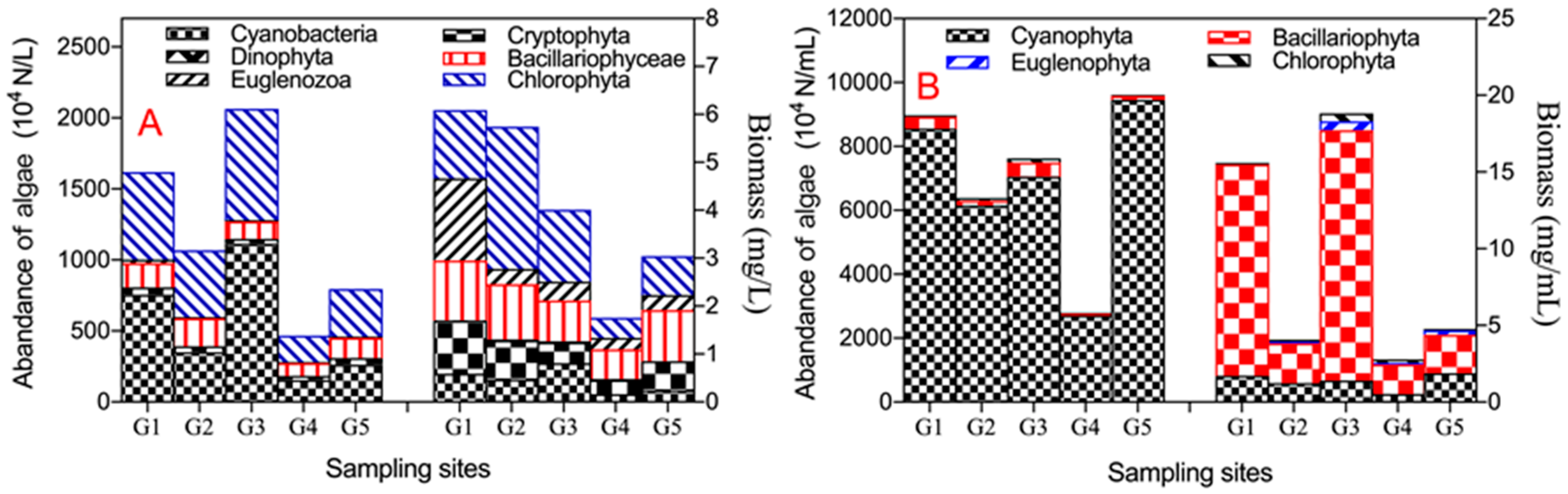
Figure 4.
The seasonal changes of abundance and biomass of planktic (A) and epipelic algae (B). Notes: the left bars are the abundance of planktic algae expressed with left axis, and the right bars are the biomass of planktic algae expressed with right axis.
Figure 4.
The seasonal changes of abundance and biomass of planktic (A) and epipelic algae (B). Notes: the left bars are the abundance of planktic algae expressed with left axis, and the right bars are the biomass of planktic algae expressed with right axis.

Figure 5.
RDA ordination between the abundance of algae and environmental factors. Note: the G1–G5 refer to the planktic algae samples in different sites, the G21–G24 refer to the planktic algae samples in G2 site and G21 is spring sample, G22 is summer sample, G23 is autumn sample, and G24 is winter sample. The G1s–G5s refer to the epipelic algae samples in different sites, the G21s–G24s refer to the epipelic algae samples in G2 site and G21s is spring sample, G22s is summer sample, G23s is autumn sample, and G24s is winter sample. Cya: Cyanobacteria; Din: Dinophyta; Bac: Bacillariophyceae; Chl: Chlorophyta; Eug: Euglenozoa.
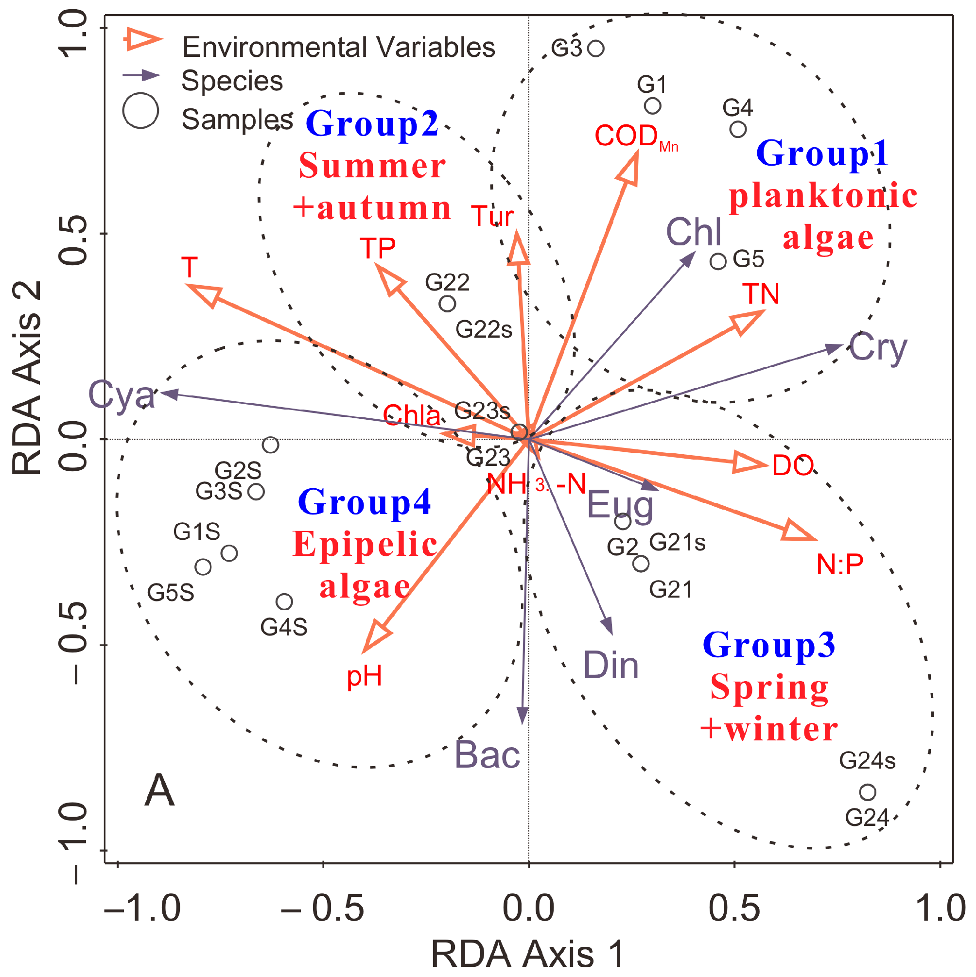
Figure 6.
Identification of environmental factors affecting the distribution of planktic algae (left) and epipelic algae (right). P, K, and S: the correlation analysis of Pearson, Kendall, and Spearman; M: multiple stepwise regression analysis; R: Redundancy analysis; T: temperature; Tur: turbidity; N:P: ratio of nitrogen and phosphorous. Cya: Cyanobacteria; Cryptophyta (Cry); Din: Dinophyta; Bac: Bacillariophyceae; Eug: Euglenozoa; Chl: Chlorophyta. The color change from green to red shows the increase of importance on the effect of algae distribution. For the calculation method see Section 2.4.


Table 1.
The seasonal changes of the abundance and biomass of the dominant planktic algae.
| Algae | Spring | Summer | Autumn | Winter | Average | ||||||
|---|---|---|---|---|---|---|---|---|---|---|---|
| A 1) | B 2) | A 1) | B 2) | A 1) | B 2) | A 1) | B 2) | A 1) | B 2) | ||
| Cyanobacteria | Anagnostidinema amphibium | 167 | 0.012 | 6580 | 0.461 | 567 | 0.004 | 0 | 0 | 1829 | 0.128 |
| Spirulina platensis | 0 | 0 | 767 | 0.153 | 417 | 0.083 | 0 | 0 | 296 | 0.059 | |
| Sum | 1530 | 0.060 | 10166 | 0.743 | 2966 | 0.227 | 117 | 0.004 | 3695 | 0.259 | |
| Cryptophyta | Cryptomonas ovata | 517 | 2.067 | 183 | 0.733 | 350 | 1.400 | 67 | 0.267 | 279 | 1.072 |
| Chroomonas acuta | 727 | 0.073 | 200 | 0.020 | 150 | 0.015 | 100 | 0.010 | 294 | 0.029 | |
| Sum | 1243 | 1.959 | 383 | 0.753 | 500 | 1.415 | 167 | 0.277 | 573 | 1.101 | |
| Dinophyta | Gymnodinium aeruginosum | 0 | 0 | 17 | 0.050 | 16.7 | 0.050 | 0 | 0 | 8.3 | 0.005 |
| Sum | 0 | 0 | 17 | 0.050 | 16.7 | 0.050 | 0 | 0 | 8.3 | 0.025 | |
| Bacillario-phyceae | Cyclotella meneghiniana | 1193 | 0.931 | 500 | 0.393 | 917 | 0.715 | 697 | 0.546 | 828 | 0.646 |
| Stephanodiscus hantzschii | 680 | 1.363 | 1330 | 0.267 | 350 | 0.700 | 33 | 0.067 | 299 | 0.599 | |
| Aulacoseira granulata | 67 | 0.022 | 2617 | 0.864 | 850 | 0.281 | 167 | 0.055 | 925 | 0.305 | |
| Sum | 2110 | 2.688 | 3283 | 1.590 | 2183 | 1.836 | 983 | 0.851 | 2140 | 1.741 | |
| Euglenozoa | Euglena viridis | 67 | 0.467 | 50 | 0.350 | 83 | 0.817 | 0 | 0 | 58 | 0.408 |
| Sum | 573 | 1.520 | 67 | 0.417 | 166.7 | 0.950 | 33 | 0.067 | 210 | 0.738 | |
| Chlorophyta | Pandorina morum | 0 | 0 | 2667 | 4.000 | 200 | 0.300 | 0 | 0 | 717 | 1.075 |
| Oocystis lacustris | 633 | 0.317 | 467 | 0.233 | 283 | 0.142 | 217 | 0.108 | 400 | 0.200 | |
| Scenedesmus sp. 3) | 1133 | 0.227 | 1700 | 0.340 | 667 | 0.133 | 333 | 0.067 | 960 | 0.192 | |
| Sum | 4637 | 1.686 | 9267 | 5.880 | 3400 | 0.770 | 1116 | 0.253 | 4605 | 2.147 | |
Note: 1) A: abundance, unit: 1000 N/L; 2) B: biomass, unit: mg/L. 3) Scenedesmus sp. include Scenedesmus quadricauda and Scenedesmus bijuga.
Table 2.
The seasonal changes of the abundance and biomass of the dominant species of epipelon.
| Algae | Spring | Summer | Autumn | Winter | Average | ||||||
|---|---|---|---|---|---|---|---|---|---|---|---|
| A 1) | B 2) | A 1) | B 2) | A 1) | B 2) | A 1) | B 2) | A 1) | B 2) | ||
| Cyano- bacteria | Anagnostidinema amphibium | 250 | 0.050 | 4209 | 0.838 | 1625 | 0.325 | 0 | 0 | 1659 | 0.331 |
| Sum | 406 | 0.096 | 5258 | 1.273 | 2700 | 0.541 | 1.4 | 0.0001 | 2091 | 0.478 | |
| Bacillario-phyceae | Cyclotella meneghiniana | 1.1 | 0.043 | 7.6 | 0.304 | 6.1 | 0.245 | 1.1 | 0.044 | 4.3 | 0.173 |
| Stephanodiscus hantzschii | 7.4 | 0.296 | 4.3 | 0.171 | 11.5 | 0.460 | 8.1 | 0.325 | 8.5 | 0.341 | |
| Aulacoseira granulata | 7.0 | 0.228 | 28.5 | 0.707 | 19.2 | 0.470 | 6.4 | 0.045 | 16.7 | 0.396 | |
| Navicula aitchelbee | 10.2 | 0.371 | 1.4 | 0.023 | 11.7 | 0.229 | 22.1 | 0.441 | 12.3 | 0.290 | |
| Fragilaria amphicephaloides | 4.6 | 0.457 | 0.7 | 0.066 | 0.5 | 0.050 | 1.8 | 0.177 | 2.1 | 0.205 | |
| Nitzschia palea | 7.6 | 0.303 | 1.5 | 0.044 | 1.0 | 0.030 | 10.2 | 0.803 | 5.5 | 0.322 | |
| Gomphonema parvulum | 27.0 | 0.540 | 0.6 | 0.011 | 0.6 | 0.011 | 46.6 | 0.931 | 20.4 | 0.407 | |
| Pinnularia microstauron | 1.7 | 0.167 | 1.6 | 0.245 | 0.5 | 0.050 | 2.8 | 0.283 | 1.8 | 0.203 | |
| Tabellaria fenestrata | 2.8 | 0.225 | 0.8 | 0.083 | 0.8 | 0.083 | 4.3 | 0.344 | 2.4 | 0.201 | |
| Sum | 84.5 | 2.887 | 52.5 | 1.791 | 85.9 | 2.664 | 140.5 | 4.152 | 90.8 | 2.874 | |
Note: 1) A: abundance, unit: 10,000 N/mL; 2) B: biomass, unit: mg/mL.
Table 3.
Correlation analysis between algae and environmental factors (n = 9).
| Planktic Algae | DO | CODMn | NH3-N | TN | TP | Chl-a | T | Tur | pH | N:P | |
| Cya2) | P 1) | −0.06 | 0.42 | −0.11 | 0.45 | 0.58 | 0.33 | 0.61 *3) | 0.03 | −0.23 | −0.38 |
| K | 0.00 | 0.28 | −0.06 | 0.28 | 0.46 * | 0.28 | 0.44 * | 0.17 | −0.06 | −0.39 | |
| S | −0.08 | 0.33 | 0.02 | 0.40 | 0.61 * | 0.37 | 0.50 | 0.15 | −0.03 | −0.50 | |
| Cry | P | 0.55 | −0.01 | −0.01 | −0.38 | −0.36 | 0.59 * | 0.05 | −0.04 | −0.03 | 0.22 |
| K | 0.06 | −0.11 | −0.11 | −0.44 * | −0.29 | 0.22 | 0.06 | 0.00 | 0.11 | −0.11 | |
| S | 0.17 | −0.18 | −0.30 | −0.67 * | −0.39 | 0.33 | 0.13 | 0.03 | 0.15 | −0.10 | |
| Din | P | −0.01 | −0.43 | −0.76 ** | −0.33 | −0.22 | 0.15 | 0.74 * | −0.40 | 0.52 | 0.02 |
| K | −0.09 | −0.09 | −0.34 | 0.15 | 0.10 | 0.09 | 0.65 * | −0.28 | 0.46 * | −0.09 | |
| S | −0.13 | −0.20 | −0.45 | 0.17 | 0.10 | 0.14 | 0.78 ** | −0.30 | 0.57 | −0.13 | |
| Bac | P | 0.56 | −0.44 | −0.83 ** | −0.19 | −0.45 | 0.73 * | 0.77 ** | −0.46 | 0.29 | 0.40 |
| K | 0.33 | −0.39 | −0.61 * | −0.39 | −0.34 | 0.50 * | 0.44 * | −0.39 | 0.50 * | 0.28 | |
| S | 0.47 | −0.50 | −0.75 ** | −0.32 | −0.47 | 0.57 | 0.57 | −0.43 | 0.67 * | 0.30 | |
| Eug | P | 0.43 | 0.02 | 0.16 | −0.30 | −0.27 | 0.45 | −0.09 | −0.15 | −0.23 | 0.16 |
| K | 0.11 | 0.06 | −0.06 | −0.28 | −0.11 | 0.28 | 0.00 | −0.06 | 0.06 | −0.17 | |
| S | 0.15 | 0.08 | 0.02 | −0.33 | −0.13 | 0.35 | −0.02 | −0.02 | −0.02 | −0.30 | |
| Chl | P | 0.27 | 0.27 | −0.30 | 0.35 | 0.32 | 0.63 * | 0.708 * | −0.08 | −0.12 | −0.13 |
| K | 0.28 | 0.22 | 0.00 | 0.33 | 0.29 | 0.56 * | 0.28 | 0.11 | 0.00 | −0.11 | |
| S | 0.35 | 0.33 | −0.05 | 0.37 | 0.38 | 0.72 * | 0.33 | 0.13 | −0.03 | −0.22 | |
| Epipelic algae | DO | CODMn | NH3-N | TN | TP | Chl-a | T | Tur | pH | N:P | |
| Cya | P | −0.62 * | −.33 | −0.20 | −0.63 * | 0.25 | 0.27 | 0.70 * | 0.27 | 0.16 | −0.66 * |
| K | −0.47 * | −0.20 | −0.14 | −0.42 | 0.34 | 0.03 | 0.46 * | 0.42 | 0.15 | −0.42 | |
| S | −0.57 | −0.21 | −0.17 | −0.59 * | 0.49 | 0.05 | 0.55 | 0.47 | 0.20 | −0.64 * | |
| Bac | P | −0.47 | −0.50 | 0.03 | −0.60 * | 0.16 | −0.38 | 0.12 | 0.37 | 0.22 | −0.55 |
| K | −0.32 | −0.39 | 0.22 | −0.61 * | 0.20 | −0.50 * | −0.08 | 0.11 | 0.21 | −0.44 * | |
| S | −0.36 | −0.55 | 0.27 | −0.70 * | 0.28 | −0.63 * | −0.14 | 0.17 | 0.22 | −0.60 * | |
| Eug | P | −0.52 | −0.27 | −0.07 | −0.54 | 0.44 | −0.17 | 0.45 | 0.41 | 0.32 | −0.69 * |
| K | −0.24 | −0.15 | −0.09 | −0.32 | 0.29 | 0.03 | 0.29 | 0.32 | 0.13 | −0.49 * | |
| S | −0.33 | −0.19 | −0.17 | −0.46 | 0.39 | 0.07 | 0.41 | 0.35 | 0.16 | −0.63 * | |
| Chl | P | −0.49 | −0.39 | 0.00 | −0.62 * | 0.46 | −0.41 | 0.36 | 0.42 | 0.36 | −0.75 * |
| K | −0.32 | −0.28 | 0.00 | −0.28 | 0.48 * | −0.28 | 0.31 | 0.11 | 0.45 | −0.56 * | |
| S | −0.39 | −0.43 | −0.03 | −0.55 | 0.60 * | −0.43 | 0.44 | 0.17 | 0.57 | −0.75 ** | |
Note: 1) P: Pearson correlation; K: Kendall’s tau B correlation; S: Spearman’s rho correlation. 2) Cya: Cyanobacteria; Din: Dinophyta; Bac: Bacillariophyceae; Chl: Chlorophyta; Eug: Euglenozoa. 3) *: Correlation is significant at the 0.05 level (1-tailed); **: Correlation is significant at the 0.01 level (1-tailed).
Table 4.
Correlation coefficients between algae and environmental factors (n = 9) from multivariate stepwise regression analysis (MSRA).
Table 4.
Correlation coefficients between algae and environmental factors (n = 9) from multivariate stepwise regression analysis (MSRA).
| DO | CODMn | NH3 | TN | TP | Chl-a | T | Tur | pH | N:P | ||
|---|---|---|---|---|---|---|---|---|---|---|---|
| Planktic algae | lgCya | −0.116 | 0.444 | −0.16 | 0.158 | 0.479 | 0.395 | 0.797 ** | 0.219 | −0.249 | −0.501 |
| lgCry | 0.409 | 0.052 | −0.101 | −0.411 | −0.254 | 0.596 * | 0.290 | 0.047 | −0.088 | 0.039 | |
| lgDin | −0.101 | −0.282 | −0.643 * | −0.244 | −0.056 | 0.096 | 0.731 * | −0.308 | 0.52 | −0.111 | |
| lgBac | 0.534 | −0.413 | −0.763 ** | −0.296 | −0.451 | 0.705 * | 0.723 * | −0.44 | 0.232 | 0.338 | |
| lgEug | 0.240 | 0.038 | 0.105 | −0.381 | −0.166 | 0.370 | 0.096 | −0.178 | −0.312 | −0.036 | |
| lgChl | 0.224 | 0.306 | −0.256 | 0.162 | 0.288 | 0.638 * | 0.730 * | 0.011 | −0.162 | −0.224 | |
| Epipelic algae | Cya | −0.621 * | −0.334 | −0.197 | −0.626 * | 0.249 | 0.272 | 0.703 * | 0.270 | 0.156 | −0.656 * |
| Bac | −0.470 | −0.503 | 0.035 | −0.603 * | 0.160 | −0.376 | 0.119 | 0.368 | 0.222 | −0.546 | |
| Eug | −0.522 | −0.272 | −0.075 | −0.540 | 0.438 | −0.167 | 0.451 | 0.408 | 0.321 | −0.685 * | |
| Chl | −0.487 | −0.388 | −0.002 | −0.620 * | 0.461 | −0.411 | 0.363 | 0.423 | 0.36 | −0.745 * | |
| Environ- mental factors | DO | 1 | |||||||||
| CODMn | −0.386 | 1 | |||||||||
| NH3 | −0.497 | 0.690 * | 1 | ||||||||
| TN | 0.021 | 0.572 | 0.277 | 1 | |||||||
| TP | −0.614 * | 0.906 ** | 0.629 * | 0.582 * | 1 | ||||||
| Chl−a | 0.840 ** | −0.023 | −0.486 | 0.180 | −0.262 | 1 | |||||
| T | 0.110 | 0.04 | −0.637 * | 0.055 | 0.079 | 0.536 | 1 | ||||
| Tur | −0.37 | 0.780 ** | 0.448 | 0.345 | 0.615 * | −0.089 | 0.047 | 1 | |||
| pH | 0.383 | −0.594 * | −0.650 * | −0.471 | −0.554 | 0.163 | 0.141 | −0.320 | 1 | ||
| N:P | 0.825 ** | −0.718 * | −0.553 | −0.045 | −0.827 ** | 0.470 | −0.116 | −0.570 | 0.414 | 1 |
** Correlation is significant at the 0.01 level (1-tailed), * Correlation is significant at the 0.05 level (1-tailed).
Table 5.
Model summary (n = 9).
| Dependent Variable | R | R2 | Adjusted R2 | Std. Error of Estimate | F | Sig. F | Durbin-Watson | |
|---|---|---|---|---|---|---|---|---|
| Planktic algae | lgCya a,1) | 0.915 a | 0.837 | 0.783 | 0.279 | 15.434 | 0.004 | 1.913 |
| lgDin b | 0.731 b | 0.534 | 0.468 | 0.374 | 8.034 | 0.025 | 1.302 | |
| lgBac c | 0.763 c | 0.582 | 0.522 | 0.123 | 9.737 | 0.017 | 1.429 | |
| lgChl d | 0.730 d | 0.533 | 0.466 | 0.213 | 7.986 | 0.026 | 1.932 | |
| Epipelic algae | Cyae | 0.861 e | 0.742 | 0.656 | 2009.850 | 8.615 | 0.017 | 1.986 |
| Bacf | 0.603 f | 0.363 | 0.273 | 121.639 | 3.997 | 0.046 | 2.099 | |
| Eugg | 0.685 g | 0.469 | 0.393 | 1.889 | 6.171 | 0.042 | 2.081 | |
| Chlh | 0.745 h | 0.555 | 0.492 | 31.962 | 8.741 | 0.021 | 2.102 |
Note: a: Predictors: (Constant), T, NH3-N; b: Predictors: (Constant), T; c: Predictors: (Constant), NH3-N; d: Predictors: (Constant), T; e: Predictors: (Constant), T, TN; f: Predictors: (Constant), TN; g: Predictors: (Constant), N:P (ratio of nitrogen and phosphorus); h: Predictors: (Constant), N:P. 1) Cya: Cyanobacteria; Din: Dinophyta; Bac: Bacillariophyceae; Chl: Chlorophyta; Eug: Euglenozoa.
Table 6.
Coefficients (n = 9).
| Dependent Variable | Model | Unstandardized Coefficients | Standardized Coefficients | t | Sig. | Collinearity Statistics | |||
|---|---|---|---|---|---|---|---|---|---|
| B | Std. Error | Beta | Tolerance | VIF | |||||
| Planktic algae | lgCya 1) | (Constant) | −1.639 | 1.209 | −1.356 | 0.224 | |||
| T | 0.133 | 0.024 | 1.168 | 5.470 | 0.002 | 0.595 | 1.681 | ||
| NH3-N | 0.345 | 0.126 | 0.583 | 2.732 | 0.034 | 0.595 | 1.681 | ||
| lgDin | (Constant) | −1.063 | 0.559 | −1.903 | 0.099 | ||||
| T | 0.071 | 0.025 | 0.731 | 2.834 | 0.025 | 1.000 | 1.000 | ||
| lgBac | (Constant) | 4.064 | 0.275 | 14.771 | 0.000 | ||||
| NH3-N | −0.134 | 0.043 | −0.763 | −3.120 | 0.017 | 1.000 | 1.000 | ||
| lgChl | (Constant) | 2.723 | 0.318 | 8.557 | 0.000 | ||||
| T | 0.041 | 0.014 | 0.730 | 2.826 | 0.026 | 1.000 | 1.000 | ||
| Epipelic algae | Cya | (Constant) | 4965.604 | 5195.977 | 0.956 | 0.376 | |||
| T | 343.227 | 120.476 | 0.603 | 2.849 | 0.029 | 0.961 | 1.040 | ||
| TN | −1137.081 | 473.557 | −0.508 | −2.401 | 0.053 | 0.961 | 1.040 | ||
| Bac | (Constant) | 600.277 | 220.626 | 2.721 | 0.030 | ||||
| TN | −56.186 | 28.103 | −0.603 | −1.999 | 0.086 | 1.000 | 1.000 | ||
| Eug | (Constant) | 8.040 | 2.236 | 3.595 | 0.009 | ||||
| N:P 2) | −0.173 | 0.070 | −0.685 | −2.484 | 0.042 | 1.000 | 1.000 | ||
| Chl | (Constant) | 149.144 | 37.844 | 3.941 | 0.006 | ||||
| N:P | −3.482 | 1.178 | −0.745 | −2.957 | 0.021 | 1.000 | 1.000 | ||
Note: 1) Cya: Cyanobacteria; Din: Dinophyta; Bac: Bacillariophyceae; Chl: Chlorophyta; Eug: Euglenozoa. 2) N:P: the ratio of nitrogen and phosphorus.
Table 7.
Collinearity Diagnostics.
| Condition Index | Variance Proportions | ||||||||
|---|---|---|---|---|---|---|---|---|---|
| Model | Dimension | Eigenvalue | (Constant) | T | NH3-N | TN | N:P | ||
| planktic algae | lgCya | 1 | 2.938 | 1.000 | 0.00 | 0.00 | 0.00 | / | / |
| 2 | 0.059 | 7.079 | 0.00 | 0.29 | 0.09 | / | / | ||
| 3 | 0.004 | 27.667 | 1.00 | 0.70 | 0.91 | / | / | ||
| lgDin | 1 | 1.975 | 1.000 | 0.01 | 0.01 | / | / | / | |
| 2 | 0.025 | 8.837 | 0.99 | 0.99 | / | / | / | ||
| lgBac | 1 | 1.989 | 1.000 | 0.01 | / | 0.01 | / | / | |
| 2 | 0.011 | 13.334 | 0.99 | / | 0.99 | / | / | ||
| lgChl | 1 | 1.975 | 1.000 | 0.01 | 0.01 | / | / | / | |
| 2 | 0.025 | 8.837 | 0.99 | 0.99 | / | / | / | ||
| Epipelic algae | Cya | 1 | 2.939 | 1.000 | 0.00 | 0.01 | / | 0.00 | / |
| 2 | 0.050 | 7.635 | 0.00 | 0.54 | / | 0.27 | / | ||
| 3 | 0.011 | 16.413 | 0.99 | 0.46 | / | 0.72 | / | ||
| Bac | 1 | 1.983 | 1.000 | 0.01 | / | / | 0.01 | / | |
| 2 | 0.017 | 10.790 | 0.99 | / | / | 0.99 | / | ||
| Eug | 1 | 1.960 | 1.000 | 0.02 | / | / | / | 0.02 | |
| 2 | 0.040 | 6.961 | 0.98 | / | / | / | 0.98 | ||
| Chl | 1 | 1.960 | 1.000 | 0.02 | / | / | / | 0.02 | |
| 2 | 0.040 | 6.961 | 0.98 | / | / | / | 0.98 | ||
Note: “/” refers to no data. Cya: Cyanobacteria; Din: Dinophyta; Bac: Bacillariophyceae; Chl: Chlorophyta; Eug: Euglenozoa.
© 2020 by the authors. Licensee MDPI, Basel, Switzerland. This article is an open access article distributed under the terms and conditions of the Creative Commons Attribution (CC BY) license (http://creativecommons.org/licenses/by/4.0/).
Share and Cite
MDPI and ACS Style
Xia, L.; Zhu, Y.; Zhao, Z. Understanding the Ecological Response of Planktic and Benthic Epipelic Algae to Environmental Factors in an Urban Rivers System. Water 2020, 12, 1311. https://doi.org/10.3390/w12051311
AMA Style
Xia L, Zhu Y, Zhao Z. Understanding the Ecological Response of Planktic and Benthic Epipelic Algae to Environmental Factors in an Urban Rivers System. Water. 2020; 12(5):1311. https://doi.org/10.3390/w12051311
Chicago/Turabian StyleXia, Liling, Yuelong Zhu, and Zhenhua Zhao. 2020. "Understanding the Ecological Response of Planktic and Benthic Epipelic Algae to Environmental Factors in an Urban Rivers System" Water 12, no. 5: 1311. https://doi.org/10.3390/w12051311
Note that from the first issue of 2016, this journal uses article numbers instead of page numbers. See further details here.