Monthly Flow Duration Curve Model for Ungauged River Basins


1
Department of Civil Engineering, Istanbul Kultur University, 34158 Istanbul, Turkey
2
Department of Civil Engineering, Istanbul Technical University, 34469 Istanbul, Turkey
*
Author to whom correspondence should be addressed.
Water 2020, 12(2), 338; https://doi.org/10.3390/w12020338
Submission received: 9 December 2019
/
Revised: 20 January 2020
/
Accepted: 22 January 2020
/
Published: 24 January 2020
(This article belongs to the Special Issue Hydrologic Modelling for Water Resources and River Basin Management)
Abstract
:Flow duration curve (FDC) is widely used in hydrology to assess streamflow in a river basin. In this study, a simple FDC model is developed for monthly streamflow data. The model consists of several steps including the nondimensionalization and then normalization in case the monthly streamflow data do not fit the normal probability distribution function. The normalized quantiles are calculated after which a back transformation is applied to the normalized quantiles to return back to the original dimensional streamflow data. In order to calculate annual streamflow of the river basin, an empirical regression equation is proposed using the drainage area and the annual total precipitation only as the input. As the final step of the model, dimensional quantiles of FDC are calculated. Ceyhan River basin in southern Turkey is chosen for the case study. Forty-two streamflow gauging stations are considered; two thirds of the gauging stations are used for the model calibration, and one third for validation. The modeled FDCs are compared to the observation and assessed with a number of performance metrics. They are found similar to the observed ones with a relatively good performance; they are good in the mid and high flow parts particularly while the low flow part of FDCs might require further detailed analysis.
1. Introduction
In the planning and management practices of water resources, there are many computational tools available to the researchers and engineers. Among them, the flow duration curve (FDC) is used to characterize the regime of the hydrological watershed. It is simply obtained from the observed streamflow time series listed in the ascending order and plotted against the corresponding duration of exceedance [1]. By the use of FDC, discharges of certain time percentages (quantiles) are determined; i.e., the upper and lower extreme events (floods and low flows) are calculated [2,3,4,5,6]. It is also possible to model the urban stormwater [7], determine the environmental flow allocation [8] and calculate the hydropower potential and water availability at hydrological watersheds [9,10,11].
Due to the extensive use of FDC in hydrology, the literature has a quite high number of studies based on different methodologies to derive FDCs at individual gauging stations or at a regional-scale. For example; regression equations using the morphology such as the drainage area and elevation of the hydrological basin were proposed [12,13,14] to establish FDC models. The probabilistic approach was used by many including Cigizoglu [15], Atieh et al. [16] and Boscarello et al. [17]. Similarly, FDC was studied by Muller et al. [18], Zhang et al. [19] and Muller and Thompson [20] through the use of analytical and statistical methods. The soft computational techniques such as the artificial neural networks, gene expression programming and geostatistical methods were also applied [21,22].
The FDC of the hydrological basin is obtained from the observed streamflow data. However, hydrological basins are not always properly gauged [23]. Therefore, regional FDCs are developed to transfer information from gauged sites to ungauged sites through the use of morphological characteristics of the hydrological basin [24], the combination of basin characteristics with probability distribution functions [25] or the development of regression or polynomial equations based on the drainage area [26,27]. The landscape and climate characteristics are also used for regional FDCs of ungauged basins [28,29]. A particular example for the dimensionless regional FDC in watersheds with no or limited data was given by Ganora et al. [30]. The comparative study of Swain and Patra [31] on the regional FDCs in ungauged basins should finally be mentioned from the literature.
Although a great experience is available in the literature on FDCs, research is still needed for ungauged basins particularly in developing countries where water resources development projects are in progress, and most of the hydrological basins are either ungauged, improperly gauged or poorly gauged. The transfer of FDC models developed for a gauged hydrological basin is not transferable to any another basin unless the basins are similar not only in terms of their hydrometeorological character but also in terms of their geomorphology [32]. With higher needs to water, smaller size river basins or subbasins within river basins, which are likely ungauged or poorly gauged, have gained importance for water resources development programs of countries under development. Therefore, studies on FDC models still emerge for ungauged river basins.
This study aims at contributing research on FDC of ungauged river basins by using hydrometeorological and topographical data of the surrounding basins. Different time scales are used in hydrological analysis and practice depending on the problem in hand. At the annual scale, the average streamflow for the river is calculated; thus, the average behavior of the river could be depicted. A better understanding of the pattern of streamflow is obtained by a monthly analysis, which has the capability of illustrating the months that contain high flows, low flows or average flows. The shape of the FDC in its upper and lower regions, which has a particular importance in evaluating the stream and basin characteristics is masked by the averaging at the annual time scale while it becomes clear when monthly streamflow data are considered. Naturally, an FDC based on monthly data provides more detailed information compared to the annual FDC. In this study, the annual FDC model of Burgan and Aksoy [33] is extended to the monthly streamflow data of the Ceyhan River basin in the Mediterranean region, the southern part of Turkey [34].
2. Flow Duration Curve Model
2.1. Steps of the Model
The FDC model is composed of the following steps schematized in Figure 1:
(a) Nondimensionalization: Time series of monthly streamflow discharge are divided by the long-term mean streamflow () and nondimensionalized at each gauging station as
in which is the nondimensional mean streamflow of month j in year i and is the observed mean streamflow (dimensional) of month j in year i.
(b) Normal distribution test: Using statistical tests, it is checked if the dimensionless discharges fit the normal distribution. A simple way to check the normality is the ratio of the average of the dimensionless discharges to their median value. A ratio changing in the range of 0.95–1.05 shows an acceptable normalization. Alternatively, the histogram of the discharges or the double probability (P–P) plot can be used. The chi-squared test is also available to check the normality of the data.
(c) Normalization: A transformation is applied to the nondimensional monthly mean streamflow to fit the time series to the normal probability distribution function. In this study,
is used where is the normalized nondimensional streamflow of month j in year i. The parameter is determined by the trial-and-error. In case no transformation is needed, = 1.
(d) Calculation of normalized quantiles: The normalized quantiles corresponding to the exceedance probability D, , is calculated as
in which and are the mean and standard deviation of the normalized streamflow, respectively, and is taken from the standard normal distribution.
(e) Back transformation of nondimensional quantiles: Given that and are known the q-quantile of exceedance probability D, , is obtained by the inverse transformation of
(f) Calculation of mean streamflow: An empirical equation, which uses the watershed drainage area (A in km2), annual precipitation (P in mm) and topographical slope of the river channel (watershed; S), was proposed in this study for calculating the long-term annual mean streamflow discharge of each river basin. A power function of
were considered in calculating the annual mean streamflow (). In Equation (5), , , and are parameters to be determined through the nonlinear regression.
(g) Calculation of dimensional quantiles: The dimensional Q-quantile of exceedance probability D, , can be determined by
for any ungauged site within the river basin.
2.2. Watershed Characteristics and Precipitation
Watershed area (A in km2), average slope of the watershed (S dimensionless) and precipitation over the watershed (P in mm) were considered in the development of the nonlinear regression equation to calculate the average streamflow. The area and slope were obtained by using the digital elevation model (DEM) of the watershed. In this study, the freely available MERIT DEM was used [35], which gives sensitive results particularly in watersheds small in size. As for the areal precipitation at the annual scale, the accumulation of the monthly precipitation data of the existing meteorological network within and surrounding the watershed was used. Precipitation (P) over the watershed was calculated by
in which N shows the number of meteorological stations, is the area (in the Thiessen polygon) represented by meteorological station i and is its precipitation.
2.3. Performance Metrics
Metrics listed in Table 1 were used to check the performance of the FDC model proposed for the monthly streamflow data. In the expressions of the performance criteria in Table 1, the following notations were applied: : observed streamflow discharge at rank i, : streamflow discharge calculated from the model at rank i, : streamflow discharge observed at 20% exceedance probability, : streamflow discharge observed at 70% exceedance probability, : streamflow discharge calculated from the model at 20% exceedance probability and : streamflow discharge calculated from the model at 70% exceedance probability. All pairs of observed and modeled streamflow were used in calculating performance metrics other than the BiasFHV, BiasFLV and SFDC for which only streamflow at 20% and 70% exceedance probabilities were considered. Yet, they show how successful the modeled FDC was in approaching the upper, the middle and lower parts of the observed FDC. It is decided how good the model performed based on the performance criteria of the metrics given in Table 2.
3. Study Area and Data
The Ceyhan River basin in the semi-arid Eastern Mediterranean Region of Turkey was selected for the case study (Figure 2). The basin is located between the north latitudes 36°33′ to 38°44′, and the east longitudes 35°15′ to 37°43′ [39]. Mountains in the basin are as high as 2500 m [40]. The southern part of the basin stays in the Cukurova Plain, which is one of the most important agricultural production areas in Turkey [41]. Forty-one percent of the total area of the basin is used actively as agricultural lands. It has a drainage area of 21,982 km2. The main river in the basin is Ceyhan that flows southerly and discharges into the Mediterranean Sea as a wide delta plain. It is 425 km-long with a mean annual streamflow of 82.9 m3/s. With its maximum that concentrates in the central part of the river basin, annual precipitation changes within a range from 278.5 to 1083.3 mm (Figure 2). On average, the river basin has an annual precipitation of 649.1 mm and an annual runoff of 341.3 mm corresponding to a runoff coefficient of 53.6% [42].
As an extension of the annual FDC model of Burgan and Aksoy [33], the proposed monthly model differs from the annual FDC model with its application area, which was taken as only the Ceyhan River basin [34]. The use of data only from the Ceyhan River basin allows one to concentrate on a more homogeneous hydrological behavior, which is needed to derive a better performed regression equation, the key element of the model. In the monthly model, also Thiessen polygon was used for calculating the areal precipitation whereas the nearest meteorological station was taken to represent each streamflow gauging station at the annual FDC model.
Data that are composed of the daily streamflow and monthly precipitation records were accessed from hydrometric stations of the General Directorate of State Hydraulic Works (DSI) and meteorological stations of the General Directorate of Meteorology (MGM) of Turkey. Monthly precipitation data are available (Table 3) for 25 meteorological stations spatially distributed within and surrounding the Ceyhan River basin (Figure 2). Annual total precipitation that represents each streamflow gauging station was calculated from the Thiessen polygon established for the meteorological stations. As for the streamflow data, monthly mean streamflow was aggregated from the daily data of 42 gauging stations (each with 10 years of observation at a minimum). Two thirds of the gauging stations were used for the model calibration and one third for its validation (Table 4). For the validation gauging stations, extra attention was paid as they vary in the size of their drainage area; i.e., gauging stations with different sizes of drainage area were used. Gauging stations were therefore divided into two groups with a drainage area less or more than 300 km2, an arbitrarily selected size. It is seen from Figure 3 that 32 out of 42 gauging stations have a drainage area less than 300 km2 while the rest of the gauging stations are larger in size. Eleven out of 14 validation gauging stations are in a size smaller than 300 km2 while the remaining three have a drainage area larger than 300 km2. It is particularly considered that gauging stations selected for the calibration and validation extend over the Ceyhan River basin (Figure 2). It is important to emphasize that streamflow data were taken from hydrometric stations with almost or practically no anthropogenic changes; i.e., when a reservoir exists at the upstream part of any gauging station, data after the reservoir were not considered but only data before the reservoir were used.
4. Results and Discussion
4.1. Application
The model was applied on precipitation and streamflow data detailed in Section 3 with summary characteristics in Table 3 and Table 4. Details of the application on an example gauging station are as follows for each step of the model:
(a) Nondimensionalization: First, streamflow data were nondimensionalized by using Equation (1); i.e., streamflow discharge at each month is divided by the long-term average streamflow discharge of the gauging station. In order to demonstrate how the model is applied at this step, an example is shown by using data from gauging station D20A019, which had an observation period extending over 10 years from 1963 to 1972 (Table 5).
(b) Normalization: In this step, the non-normal data were converted into normal distribution. Within the 8664 station-month streamflow data in Table 4, 31 station-months only were recorded as zero, which were excluded from the normalization. The average and standard deviation of the non-zero monthly streamflow discharge records were calculated after which θ = 0.166 was obtained by the trial-and-error to make the data set normal. It is seen from the histogram in Figure 4 and the P–P plot in Figure 5 that the data were normalized properly. The ratio of was calculated as 1.01, which simply shows the goodness-of-fit of the normal distribution to the data after the transformation. The transformed data were further checked by the test that approved the normalization. All these checks and tests showed that the normalization was achieved. In Table 6, the nondimensional monthly streamflow data are given for the example gauging station (D20A019).
(c) Calculation of normal quantiles: The standard normal variable was given for different exceedance probabilities in Table 7. Given that the mean and standard deviation are available, the transformed streamflow of any exceedance probability could be calculated by Equation (3), = 1.05 for = 25% exceedance probability as an example.
(d) Back transformation of nondimensional quantiles: Equation (4) was used for the back transformation of the nondimensional streamflow discharge data (; Table 7); = 1.31 for = 25% as an example (Table 8, Figure 6).
(e) Calculation of the mean streamflow: The dimensional quantiles of FDC can be calculated by using the empirical regression equation, which is developed between the mean streamflow and watershed characteristics among which the drainage area and slope of each watershed were taken into account together with precipitation. Following equations were obtained to alternate each other in calculating the average streamflow discharge of the Ceyhan River basin.
In calculating the average streamflow discharge at the calibration stage, Equation (12) was found the best based on the determination coefficient (R2) and the root mean square error (RMSE) while Equation (10) performed the best based on the mean absolute error (MAE; Table 9). For the validation stage, however, Equation (10) performed better than all others although the performance metrics did not differ from each other considerably. The similar performance of the alternative equations could bring the concept of the equifinality to mind [43], yet, this is not an issue to be considered here. Instead, the simplest regression equation in terms of parameterization was found the most successful in reproducing the average streamflow discharge. Not only because of this reason but also due to its parsimonious structure in terms of parameters and the number of inputs, Equation (10) was preferred in this study. The fitted curve based on Equation (10) is plotted in Figure 7. The calculated streamflow discharges of each gauging station were compared with their counterparts as in Figure 8 from which a good fit was observed.
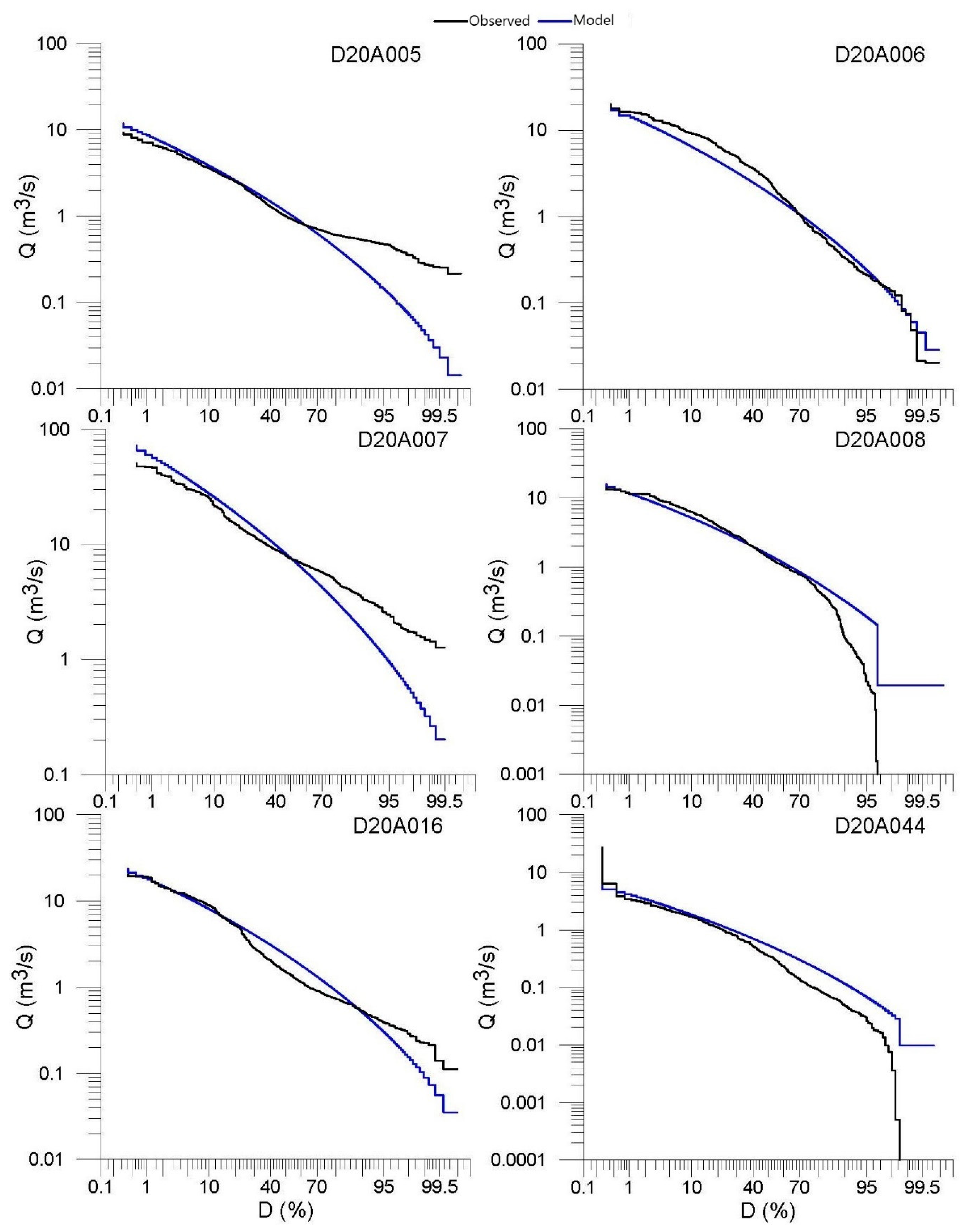
(f) Calculation of dimensional quantiles: Any dimensional discharge () corresponding to the exceedance probability can be calculated by Equation (6) using the dimensionless discharge corresponding to the same exceedance probability () and the average streamflow () calculated from Equation (10). This was applied on the validation gauging stations of the Ceyhan River basin to obtain their monthly FDCs as in Figure 9.
4.2. Discussion
In this study, in order to prove that the model is applicable to ungauged river basins, a monthly streamflow data set composed of 42 hydrometric stations was chosen from the Ceyhan River basin in southern Turkey as detailed above. FDCs of the model were compared to the observed FDCs of the gauged hydrometric stations, which were particularly chosen to show the similarity between the modeled and observed FDCs. Once the similarity is satisfied, the model can be proposed to develop FDC at any un-gauged site. This was the way in how the model was validated in this study.
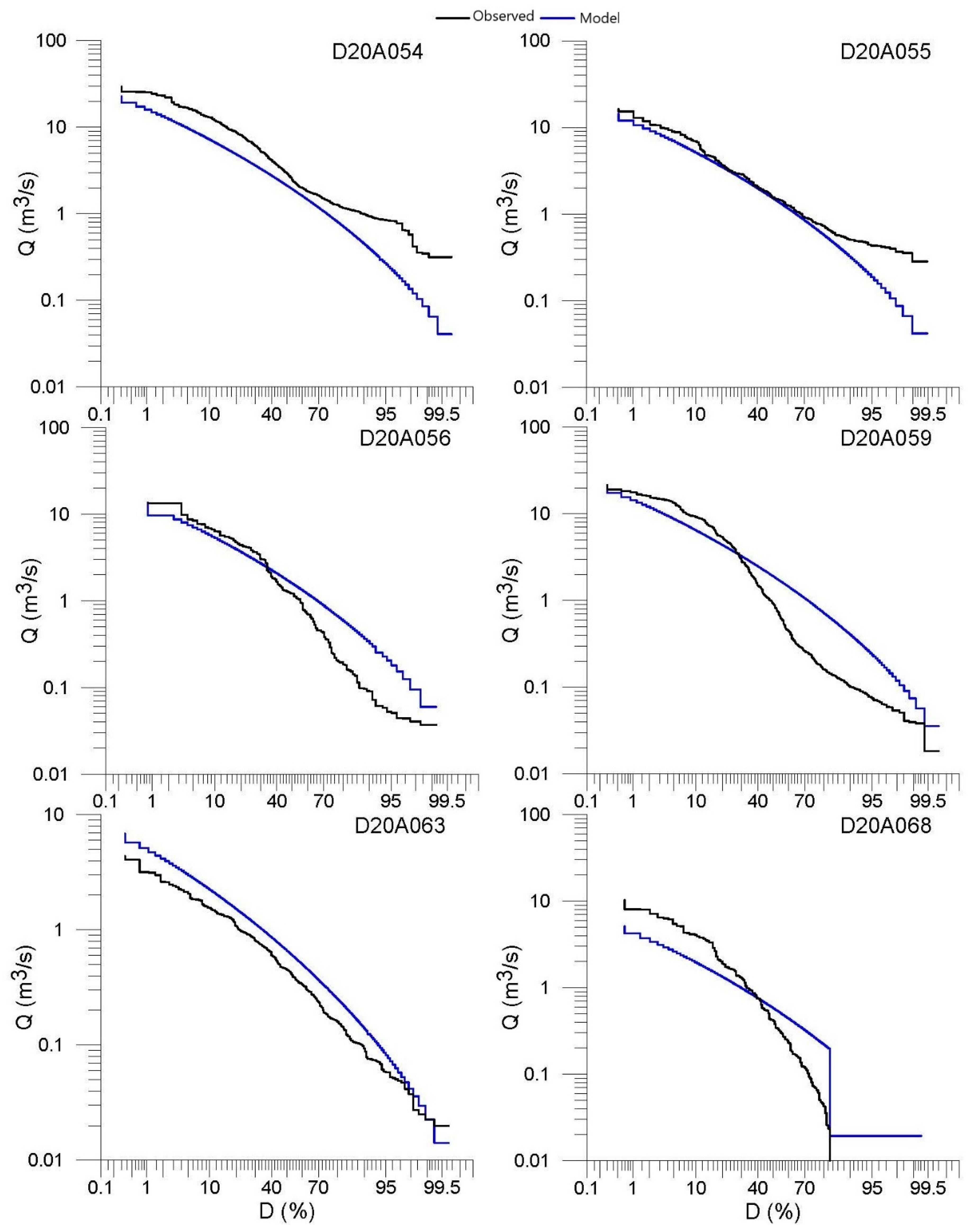
Figure 9 shows FDCs for the validation gauging stations (14 in total) for which performance metrics were obtained as in Table 10. When FDCs in Figure 9 were taken into account together with the performance criteria in Table 10, the general result that came out was that the methodology performed quite well for the validation gauging stations. This was clear particularly due to the performance criteria in Table 10, which were almost all either very good, good or adequate except for the VE in one station (D20A063) and BiasFLV in four (D20A044, D20A056, D20A059 and D20A068). The total number of inadequate cases was five out of 98 when the number of gauging stations and number of performance metrics were considered together. It is important to note also that BiasFLV is a performance metric for the lower end of the FDC where flow is quite low. Therefore, even if BiasFLV shows an inadequate performance in these particular stations, the deviation from the observation in terms of the streamflow volume is not substantial but ignorable.
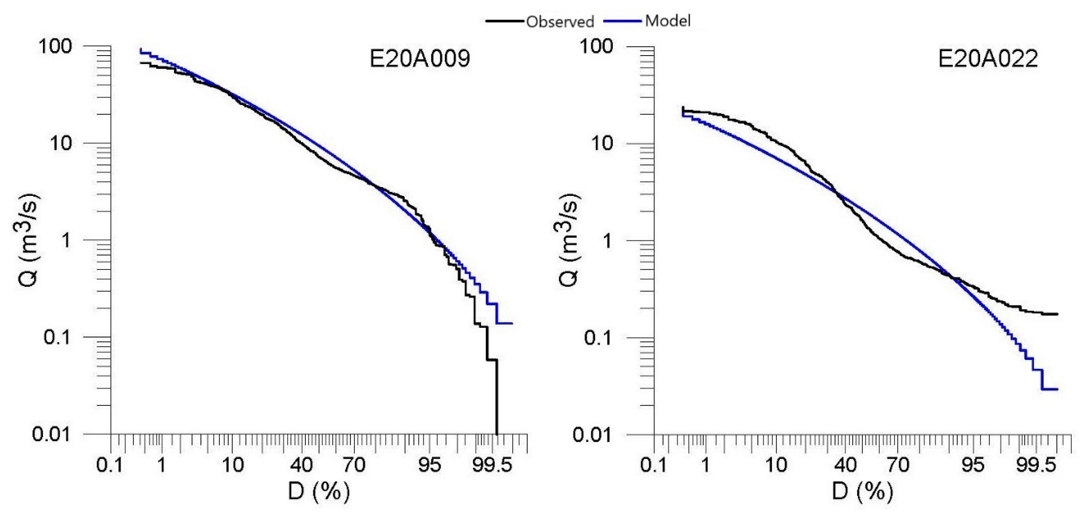
When results were analyzed, FDCs were generally considered successful as a whole and at once. However, the part-by-part analysis of FDCs is quite beneficial particularly for the lower tail with low flows. It is then possible to get more detail of the FDC. This was the case here particularly when the lower tail of the FDC did not seem to be satisfactory. The deviation was clear for exceedance probabilities higher than 70% in gauging stations D20A005, D20A007, D20A054 and D20A055. However, when BiasFLV, the performance metric applicable to the lower tail of the FDC was checked in Table 10, it was seen that it stayed in the range of “very good”, which means the visual deviation in these particular gauging stations did not necessarily mean a large-volume error. On the other hand, although the lower-tail demonstrated an “inadequate” performance in terms of the BiasFLV for gauging stations D20A044, D20A056, D20A059 and D20A068, the visual disagreement in Figure 9 was not as clear as in the above-mentioned gauging stations. The inadequate performance for the lower tail of the flow duration curve in these particular stations might be ignored; because the difference between the observed and the modeled streamflow volumes was not that substantial as the discharge was quite small. In gauging station E20A009, which is one of the two gauging stations where streamflow was intermittent, the performance metrics were found very satisfactory for the FDC. Nevertheless, in the second intermittent streamflow gauging station (D20A044), a deviation was seen between the observation and the model as this particular station had a very low streamflow discharge. This discussion can also be based on the fact that the deviation between the lower tails of the modeled and observed FDCs increased with the degree of intermittency of the river due to higher between-year variability of the FDCs in drier rivers than the wet rivers [1]. It should also be noted that logarithmic and probabilistic scales were used in the vertical and horizontal axes in Figure 9, respectively, that might exaggerate the deviation visually.
When the generalization of the results was needed, it could be seen that the modeled FDCs were underestimated for some gauging stations while they were overestimated for others. It is also seen that FDCs could behave differently in different parts; i.e., an FDC that underestimates the upper tail of the FDC might overestimate the lower tail or vice versa. This could be connected with the lumped behavior of the empirical regression equation in which the calibration gauging stations were all combined and forced to be represented by one free variable and two parameters only. Only one free variable existed in the regression equation as the basin drainage area and precipitation were used in their multiplicative form. Yet, results of the regression equation were considered acceptable.
The basic aim of this study was to develop a flow duration curve model for ungauged sites at the monthly time step. As a pre-requisite, the model needs a regression equation that links the long-term mean streamflow of the river basin to the multiplicative form of its drainage area and precipitation. The former can simply be delineated and calculated by modern geographic information systems technology while the latter is generally available or it can be obtained from areal distribution maps of precipitation. With the existence and relatively easy availability of drainage area and precipitation, the FDC model is applicable to any ungauged site within a river basin, conditional that a regression equation calculating streamflow from the drainage area and precipitation is given. The performance of the regression model is at the utmost importance. It is expected that the smaller the river basin, the better the performance of the regression equation. In this sense, the model can generally be used for smaller-size ungauged sub-basins surrounded by larger gauged river basins. However, the model could still be considered a solution to the problem of the FDC development for ungauged basins, one of the most important unsolved problems in hydrology [23,44].
5. Conclusions
A monthly FDC model was presented in this study. The normalized nondimensional monthly streamflow data were used in the model, which had an empirical regression equation based on the multiplicative form of the drainage area and precipitation as independent variables to calculate the mean streamflow of the basin. The slope of the basin was also considered as an independent variable in the regression equation, yet, it did not provide an extra improvement. The FDC model was applied on almost 14,000 station-month data from 42 stream gauges in the Ceyhan River basin in southern Turkey.
It is seen from the results of the study that a deviation was unavoidable in the lower tail of FDCs where the model overestimated the flow. This was more pronounced in the streamflow gauging stations with lower low flow values, which made the deviation less important as the error in terms of volume became negligible. The deviation in the lower part of the FDC could be linked to the higher between-year variability of intermittent river. The model was found however better and even satisfactory in the upper and middle parts (between 0% and 70% of the time of exceedances) of the FDCs. Therefore, rather than the upper and middle parts of the FDC, it is important to consider the lower part for a separate and further analysis.
When a general look was made at the results, it was found that the model was promising although it seemed that it had a low performance in some gauging stations. This was particularly the case when the gauging station deviated from the average hydrological behavior of the basin. The less similarity to the average hydrological behavior was reflected by the empirical regression equation established between the streamflow and watershed characteristics, the drainage area and precipitation. The regression equation produced FDCs better approaching to the observation in gauging stations, which had a behavior similar to the average of the river basin. In other words, the FDC model was expected to perform better with an empirical regression equation better approaching the mean streamflow of the river basin. Therefore, the regression equation is the key issue to be further analyzed for the FDC model.
The FDC model is applicable to any ungauged site within a river basin for which data exist. It is simple as only the streamflow and precipitation data are needed together with the watershed drainage area. Results seem acceptable, encouraging, even promising. However, in order to generalize the applicability of the model, rigorous tests might be needed through additional case studies from geographical regions under different climatological conditions. A time interval shorter than a month (a day for example) is considered beneficial in the future development direction of the proposed model.
Author Contributions
Conceptualization, H.I.B. and H.A.; Data Curation, H.A. and H.I.B.; Formal Analysis, H.I.B. and H.A.; Funding Acquisition, H.A.; Investigation, H.I.B. and H.A.; Methodology, H.A. and H.I.B.; Software, H.I.B.; Supervision, H.A.; Visualization, H.I.B.; Writing—Original Draft Preparation, H.I.B. and H.A.; Writing—Review and Editing, H.A. and H.I.B. All authors have read and agreed to the published version of the manuscript.
Funding
This study is a part of PhD thesis of the first author under the supervision of the second. The study was supported by Research Fund of Istanbul Technical University under project Flow Duration Curve Model for Ungauged Intermittent Rivers (Project no. 39334).
Acknowledgments
Streamflow data were provided by State Hydraulic Works (DSI), precipitation data by General Directorate of Meteorology (MGM) and State Hydraulic Works (DSI) of Turkey.
Conflicts of Interest
The authors declare no conflict of interest.
References
- Castellarin, A.; Botter, G.; Hughes, D.A.; Liu, S.; Ouarda, T.B.M.J.; Parajka, J.; Post, D.A.; Sivapalan, M.; Spence, C.; Viglione, A.; et al. Prediction of flow duration curves in ungauged basins. In Runoff Prediction in Ungauged Basins: Synthesis across Processes, Places and Scales, 1st ed.; Bloeschl, G., Sivapalan, M., Wagener, T., Viglione, A., Savenije, H., Eds.; Cambridge University Press: Cambridge, UK, 2013; pp. 135–162. [Google Scholar]
- Vogel, R.M.; Fennessey, N.M. Flow-duration curves I: New interpretation and confidence intervals. J. Water Res. Plan. Manag. 1994, 120, 485–504. [Google Scholar] [CrossRef]
- Vogel, R.M.; Fennessey, N.M. Flow duration curves II: A review of applications in water resources planning. Water Resour. Bull. Am. Water Resour. Assoc. 1995, 31, 1029–1039. [Google Scholar] [CrossRef]
- Smakhtin, V.U. Low flow hydrology: A review. J. Hydrol. 2001, 240, 147–186. [Google Scholar] [CrossRef]
- Castellarin, A.; Galeati, G.; Brandimarte, L.; Montanari, A.; Brath, A. Regional flow-duration curves: Reliability for ungauged basins. Adv. Water Resour. 2004, 27, 953–965. [Google Scholar] [CrossRef]
- Lane, P.N.J.; Best, A.E.; Hickel, K.; Zhang, L. The response of flow duration curves to afforestation. J. Hydrol. 2005, 310, 253–265. [Google Scholar] [CrossRef]
- Petrucci, G.; Rodriguez, F.; Deroubaix, J.; Tassin, B. Linking the management of urban watersheds with the impacts on the receiving water bodies: The use of flow duration curves. Water Sci. Technol. 2014, 70, 127–135. [Google Scholar] [CrossRef]
- Yang, W.; Yang, Z. Analyzing hydrological regime variability and optimizing environmental flow allocation to lake ecosystems in a sustainable water management framework: Model development and a case study for China’s Baiyangdian Watershed. J. Hydrol. Eng. 2014, 19, 993–1005. [Google Scholar] [CrossRef]
- Quimpo, R.G.; Alejandrino, A.A.; McNally, T.A. Regionalized flow duration for Philippines. J. Water Resour. Plan. Manag. 1983, 109, 320–330. [Google Scholar] [CrossRef]
- Baltas, E.A. Development of a regional model for hydropower potential in Western Greece. Glob. NEST J. 2012, 14, 442–449. [Google Scholar]
- Kim, J.T.; Kim, G.B.; Chung, I.M.; Jeong, G.C. Analysis of flow duration and estimation of increased groundwater quantity due to groundwater dam construction. J. Eng. Geol. 2014, 24, 91–98. [Google Scholar] [CrossRef] [Green Version]
- Singh, K.P. Model flow duration and streamflow variability. Water Resour. Res. 1971, 7, 1031–1036. [Google Scholar] [CrossRef]
- Dingman, S.L. Synthesis of flow duration curves for unregulated streams in New Hampshire. Water Resour. Bull. Am. Water Resour. Assoc. 1978, 14, 1481–1502. [Google Scholar] [CrossRef]
- Singh, R.D.; Mishra, S.K.; Chowdhary, H. Regional flow duration models for large number of ungauged Himalayan catchments for planning microhydro projects. J. Hydrol. Eng. 2001, 6, 310–316. [Google Scholar] [CrossRef]
- Cigizoglu, H.K. A method based on taking the average of probabilities to compute the flow duration curve. Hydrol. Res. 2000, 31, 187–206. [Google Scholar] [CrossRef]
- Atieh, M.; Gharabaghi, B.; Rudra, R. Entropy-based neural networks model for flow duration curves at ungauged sites. J. Hydrol. 2015, 529, 1007–1020. [Google Scholar] [CrossRef]
- Boscarello, L.; Ravazzani, G.; Cislaghi, A.; Mancini, M. Regionalization of flow-duration curves through catchment classification with streamflow signatures and physiographic–climate indices. J. Hydrol. Eng. 2016, 21, 05015027. [Google Scholar] [CrossRef]
- Muller, M.F.; Dralle, D.N.; Thompson, S.E. Analytical model for flow duration curves in seasonally dry climates. Water Resour. Res. 2014, 50, 5510–5531. [Google Scholar] [CrossRef] [Green Version]
- Zhang, Y.; Vaze, J.; Chiew, F.H.S.; Li, M. Comparing flow duration curve and rainfall–runoff modelling for predicting daily runoff in ungauged catchments. J. Hydrol. 2015, 525, 72–86. [Google Scholar] [CrossRef]
- Muller, M.F.; Thompson, S.E. Comparing statistical and process-based flow duration curve models in ungauged basins and changing rain regimes. Hydrol. Earth Syst. Sci. 2016, 20, 669–683. [Google Scholar] [CrossRef] [Green Version]
- Pugliese, A.; Farmer, W.H.; Castellarin, A.; Arcfield, S.A.; Vogel, R.M. Regional flow duration curves: Geostatistical techniques versus multivariate regression. Adv. Water Res. 2016, 96, 11–22. [Google Scholar] [CrossRef]
- Atieh, M.; Taylor, G.; Sattar, A.M.A.; Gharabaghi, B. Prediction of flow duration curves for ungauged basins. J. Hydrol. 2017, 545, 383–394. [Google Scholar] [CrossRef]
- Hrachowitz, M.; Savenije, H.H.G.; Bloschl, G.; McDonnell, J.J.; Sivapalan, M.; Pomeroy, J.W.; Arheimer, B.; Blume, T.; Clark, M.P.; Ehret, U.; et al. A decade of Predictions in Ungauged Basins (PUB)—A review. Hydrol. Sci. J. 2013, 58, 1198–1255. [Google Scholar] [CrossRef]
- Mimikou, M.; Kaemaki, S. Regionalization of flow duration characteristics. J. Hydrol. 1985, 82, 77–91. [Google Scholar] [CrossRef]
- Wittenberg, H. Regional Analysis of Flow Duration Curves; No. 187; IAHS Publications: Wallingford, UK, 1989; pp. 213–220. [Google Scholar]
- Yu, P.S.; Yang, T.C. Synthetic regional flow duration curve for southern Taiwan. Hydrol. Process. 1996, 10, 373–391. [Google Scholar] [CrossRef]
- Yu, P.S.; Yang, T.C.; Wang, Y.C. Uncertainty analysis of regional flow duration curves. J. Water Resour. Plan. Manag. 2002, 128, 424–430. [Google Scholar] [CrossRef]
- Mohamoud, Y.M. Prediction of daily flow duration curves and streamflow for ungauged catchments using regional flow duration curves. Hydrol. Sci. J. 2008, 53, 706–724. [Google Scholar] [CrossRef]
- Doulatyari, B.; Betterle, A.; Basso, A.; Biswal, B.; Schirmer, M.; Botter, G. Predicting streamflow distributions and flow duration curves from landscape and climate. Adv. Water Resour. 2015, 83, 285–298. [Google Scholar] [CrossRef]
- Ganora, D.; Claps, P.; Laio, F.; Viglione, A. An approach to estimate nonparametric flow duration curves in ungauged basins. Water Resour. Res. 2009, 45, W10418. [Google Scholar] [CrossRef]
- Swain, J.B.; Patra, K.C. Streamflow estimation ungauged catchments using regional flow duration curve: Comparative study. J. Hydrol. Eng. 2017, 22, 04017010. [Google Scholar] [CrossRef]
- Wagener, T.; Sivapalan, M.; Troch, P.; Woods, R. Catchment classification and hydrologic similarity. Geogr. Compass 2007, 1, 901–931. [Google Scholar] [CrossRef]
- Burgan, H.I.; Aksoy, H. Annual flow duration curve model for ungauged basins. Hydrol. Res. 2018, 49, 1684–1695. [Google Scholar] [CrossRef]
- Burgan, H.I. Flow Duration Curve MOdel for Ungauged Intermittent Rivers. Ph.D. Thesis, Hydraulics and Water Resources Program, Department of Civil Engineering, Graduate School of Science, Engineering and Technology, Istanbul Technical University, Istanbul, Turkey, July 2019; 164p. [Google Scholar]
- MERIT DEM: Multi-Error-Removed Improved-Terrain DEM. Available online: http://hydro.iis.u-tokyo.ac.jp/~yamadai/MERIT_DEM (accessed on 31 December 2017).
- Pfannerstill, M.; Guse, B.; Fohrer, N. Smart low flow signature metrics for an improved overall performance evaluation of hydrological models. J. Hydrol. 2014, 510, 447–458. [Google Scholar] [CrossRef]
- Ridolfi, E.; Kumar, H.; Bardossy, A. A methodology to estimate flow duration curves at partially ungauged basins. Hydrol. Earth Syst. Sci. Diss. 2018, 1–30. [Google Scholar] [CrossRef]
- Moriasi, D.N.; Arnold, J.G.; Van Liew, M.W.; Bingner, R.L.; Harmel, R.D.; Veith, T.L. Model evaluation guidelines for systematic quantification of accuracy in watershed simulations. Trans. ASABE 2007, 50, 885–900. [Google Scholar] [CrossRef]
- Yuce, M.I.; Esit, M.; Ciloglan Karatas, M. Hydraulic geometry analysis of Ceyhan River, Turkey. SN Appl. Sci. 2019, 1, 763. [Google Scholar] [CrossRef] [Green Version]
- Eris, E.; Aksoy, H.; Onoz, B.; Cetin, M.; Yuce, M.I.; Selek, B.; Aksu, H.; Burgan, H.I.; Esit, M.; Yildirim, I.; et al. Frequency analysis of low flows in intermittent and non-intermittent rivers from hydrological basins in Turkey. Water Sci. Technol. Water Supply 2019, 19, 30–39. [Google Scholar] [CrossRef]
- Gumus, V.; Algin, H.M. Meteorological and hydrological drought analysis of the Seyhan−Ceyhan River Basins, Turkey. Meteorol. Appl. 2017, 24, 62–73. [Google Scholar] [CrossRef]
- Aksoy, H. Surface Water. In Water Resources of Turkey, 1st ed.; Harmancioglu, N.B., Altinbilek, D., Eds.; Springer: Cham, Switzerland, 2020; pp. 127–158. [Google Scholar]
- Tu, M.C.; Smith, P. Modeling pollutant buildup and washoff parameters for SWMM based on land use in a semiarid urban watershed. Water Air Soil Pollut. 2018, 229, 121. [Google Scholar] [CrossRef]
- Bloschl, G.; Bierkens, M.F.P.; Chambel, A.; Cudennec, C.; Destouni, G.; Fiori, A.; Kirchner, J.W.; McDonnell, J.J.; Savenije, H.H.G.; Sivapalan, M.; et al. Twenty-three unsolved problems in hydrology (UPH)―a community perspective. Hydrol. Sci. J. 2019, 64, 1141–1158. [Google Scholar] [CrossRef] [Green Version]
Figure 1.
Steps of the model.

Figure 2.
Water courses, hydrometric and meteorological stations and an isohyet map of the Ceyhan River Basin in Turkey.
Figure 2.
Water courses, hydrometric and meteorological stations and an isohyet map of the Ceyhan River Basin in Turkey.

Figure 3.
Selection of the calibration and validation streamflow gauging stations based on their drainage area, A < 300 km2 (upper panel) and A > 300 km2 (lower panel).
Figure 3.
Selection of the calibration and validation streamflow gauging stations based on their drainage area, A < 300 km2 (upper panel) and A > 300 km2 (lower panel).

Figure 4.
Histogram of the nondimensional streamflow data fitted to the normal probability distribution.
Figure 4.
Histogram of the nondimensional streamflow data fitted to the normal probability distribution.

Figure 5.
The P–P plot of the dimensionless monthly streamflow data after normalization.

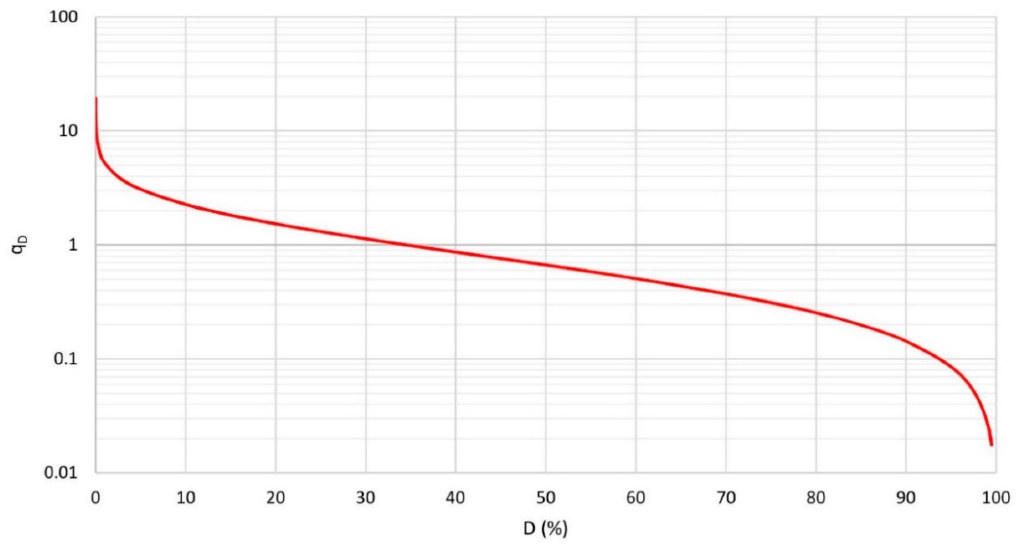
Figure 6.
The nondimensional FDC of the Ceyhan River basin.

Figure 7.
Relation between the watershed average streamflow and watershed area-precipitation (Equation (10)).
Figure 7.
Relation between the watershed average streamflow and watershed area-precipitation (Equation (10)).

Figure 8.
Observed and estimated watershed average streamflow discharge.

Figure 9.
FDC of the monthly streamflow for validation gauging stations (continued).


| Metrics | Expression | Range | Remarks |
|---|---|---|---|
| Nash-Sutcliffe Efficiency | NSE approaching 1 is better. | ||
| Root Mean Square Error | RMSE is dimensional as the variable. RMSE approaching zero is better. | ||
| Ratio of Standard Deviation | RSD approaching zero is better. | ||
| Mean Square Error | MSE approaching zero is better. | ||
| Mean Absolute Error | MAE approaching zero is better. | ||
| Relative Error | RE approaching zero is better. | ||
| Volume Error | VE approaching zero is better. | ||
| Percent Bias in FDC High-Segment Volume | BiasFHV is used for the higher part of FDC (the highest 20%) | ||
| Percent Bias in FDC Low-Segment Volume | BiasFLV is used for the lower part of FDC (the lowest 30%) | ||
| Slope of FDC | SFDC is used for the medium part of FDC (from 20% to 70%) |
Table 2.
Performance of the metrics [38].
Table 2.
Performance of the metrics [38].
| Performance | NSE | RSD | RE | BiasFHV | BiasFLV | SFDC | RMSE | MSE | MAE | VE |
|---|---|---|---|---|---|---|---|---|---|---|
| Very good | Metric approaching zero is better. | |||||||||
| Good | ||||||||||
| Adequate | ||||||||||
| Inadequate | ||||||||||
Table 3.
Monthly precipitation data used in the study.
| Number of Meteorological Stations | 25 |
| Shortest observation (years) | 12 |
| Longest observation (years) | 55 |
| Length of observation (station-month) | 10,560 |
| Average of monthly precipitation (mm) | 58.35 |
| Minimum of monthly precipitation (mm) | 0.00 |
| Maximum of monthly precipitation (mm) | 476.1 |
| Standard deviation of monthly precipitation (mm) | 61.58 |
| Coefficient of variation of monthly precipitation | 1.06 |
| Coefficient of skewness of monthly precipitation | 1.65 |
Table 4.
Characteristics of streamflow data used in the study.
| Characteristics | Calibration | Validation |
|---|---|---|
| Number of gauging stations | 28 | 14 |
| Shortest observation (years) | 10 | 10 |
| Longest observation (years) | 60 | 50 |
| Length of observation (station-month) | 8664 | 5280 |
| Average of monthly streamflow (l/s-km2) | 16.9 | 16.1 |
| Minimum of monthly streamflow (l/s-km2) | 1.29 | 0.586 |
| Maximum of monthly streamflow (l/s-km2) | 102 | 156 |
| Standard deviation of monthly streamflow (l/s-km2) | 17.8 | 20.1 |
| Coefficient of variation of monthly streamflow | 1.06 | 1.21 |
| Coefficient of skewness of monthly streamflow | 1.98 | 2.82 |
| Average drainage area (km2) | 771 | 683 |
| Drainage area of smallest watershed (km2) | 23 | 33 |
| Drainage area of largest watershed (km2) | 3374 | 1801 |
| Annual precipitation over the watershed (mm) | 403 | 372 |
| Slope of the watershed | 0.0466 | 0.0461 |
Table 5.
Nondimensionalization of monthly streamflow data (D20A019).
| Year | Month | ||
|---|---|---|---|
| 1963 | 1 | 1.567 | 0.324 |
| 1963 | 2 | 0.167 | 0.035 |
| 1963 | 3 | 12.589 | 2.607 |
| ⋮ | ⋮ | ⋮ | ⋮ |
| 1972 | 10 | 1.181 | 0.245 |
| 1972 | 11 | 1.240 | 0.257 |
| 1972 | 12 | 1.707 | 0.353 |
| (m3/s) | 4.289 |
Table 6.
Normalization of monthly streamflow data (D20A019).
| Year | Month | ||
|---|---|---|---|
| 1963 | 1 | 0.324 | 0.830 |
| 1963 | 2 | 0.035 | 0.572 |
| 1963 | 3 | 2.607 | 1.172 |
| ⋮ | ⋮ | ⋮ | ⋮ |
| 1972 | 10 | 0.245 | 0.792 |
| 1972 | 11 | 0.257 | 0.798 |
| 1972 | 12 | 0.353 | 0.841 |
Table 7.
Calculation of normal quantiles.
| 5 | 1.64 | 1.20 | 55 | −0.13 | 0.91 |
| 10 | 1.28 | 1.15 | 60 | −0.25 | 0.89 |
| 15 | 1.04 | 1.10 | 65 | −0.39 | 0.87 |
| 20 | 0.84 | 1.07 | 70 | −0.52 | 0.85 |
| 25 | 0.67 | 1.05 | 75 | −0.67 | 0.82 |
| 30 | 0.52 | 1.02 | 80 | −0.84 | 0.80 |
| 35 | 0.39 | 1.00 | 85 | −1.04 | 0.76 |
| 40 | 0.25 | 0.98 | 90 | −1.28 | 0.72 |
| 45 | 0.13 | 0.96 | 95 | −1.64 | 0.66 |
| 50 | 0.00 | 0.93 |
Table 8.
Back transformation to the nondimensional flow duration curve (FDC) of the Ceyhan River basin.
Table 8.
Back transformation to the nondimensional flow duration curve (FDC) of the Ceyhan River basin.
| 5 | 3.07 | 55 | 0.58 |
| 10 | 2.26 | 60 | 0.51 |
| 15 | 1.82 | 65 | 0.44 |
| 20 | 1.53 | 70 | 0.37 |
| 25 | 1.31 | 75 | 0.31 |
| 30 | 1.13 | 80 | 0.25 |
| 35 | 0.99 | 85 | 0.20 |
| 40 | 0.87 | 90 | 0.14 |
| 45 | 0.76 | 95 | 0.09 |
| 50 | 0.67 |
Table 9.
Performance criteria calculated for the watershed average streamflow.
| Stage | Performance Metrics | Equation | ||||
|---|---|---|---|---|---|---|
| (8) | (9) | (10) | (11) | (12) | ||
| Calibration | R2 | 0.877 | 0.916 | 0.921 | 0.891 | 0.933 |
| RMSE | 2.097 | 1.713 | 1.664 | 1.995 | 1.536 | |
| MAE | 1.372 | 1.040 | 1.023 | 1.371 | 1.050 | |
| Validation | R2 | 0.890 | 0.959 | 0.964 | 0.911 | 0.952 |
| RMSE | 1.980 | 0.998 | 0.829 | 2.233 | 0.948 | |
| MAE | 1.190 | 0.667 | 0.582 | 1.427 | 0.589 | |
Table 10.
Performance metrics for the validation streamflow gauging stations (colors refer to the performance of the model; green: very good, blue: good, yellow: adequate, red: inadequate).
Table 10.
Performance metrics for the validation streamflow gauging stations (colors refer to the performance of the model; green: very good, blue: good, yellow: adequate, red: inadequate).
| SGS | Performance Metrics | |||||||
|---|---|---|---|---|---|---|---|---|
| RSD | NSE | VE | MAE | RMSE | BiasFHV | SFDC | BiasFLV | |
| D20A005 | 0.07 | 1.00 | 0.10 | 0.44 | 0.67 | 16.88 | 12.80 | −46.82 |
| D20A006 | 0.26 | 0.93 | −0.21 | 1.14 | 1.64 | −20.56 | −22.52 | 8.96 |
| D20A007 | 0.30 | 0.91 | 0.16 | 3.54 | 5.05 | 23.60 | 60.24 | −43.92 |
| D20A008 | 0.06 | 1.00 | −0.08 | 0.47 | 0.74 | −11.22 | −12.53 | 57.76 |
| D20A016 | 0.08 | 0.99 | 0.02 | 0.44 | 0.56 | −1.14 | −18.87 | 7.93 |
| D20A044 | 0.05 | 1.00 | 0.23 | 0.23 | 0.33 | 19.32 | −30.86 | 138.11 |
| D20A054 | 0.43 | 0.82 | −0.40 | 3.11 | 4.51 | −39.58 | −16.53 | −47.60 |
| D20A055 | 0.24 | 0.94 | −0.19 | 0.79 | 1.26 | −19.10 | 1.00 | −33.96 |
| D20A056 | 0.11 | 0.99 | −0.09 | 0.64 | 0.99 | −13.67 | −38.94 | 163.61 |
| D20A059 | 0.29 | 0.92 | −0.17 | 1.39 | 2.04 | −23.90 | −53.10 | 284.57 |
| D20A063 | 0.30 | 0.91 | 0.54 | 0.51 | 0.82 | 55.13 | −6.53 | 52.25 |
| D20A068 | 0.51 | 0.74 | −0.43 | 1.10 | 1.80 | −47.50 | −49.76 | 391.92 |
| E20A009 | 0.21 | 0.95 | 0.15 | 2.77 | 4.82 | 14.82 | −1.92 | 2.92 |
| E20A022 | 0.34 | 0.88 | −0.25 | 1.72 | 2.74 | −28.64 | −32.07 | 12.20 |
© 2020 by the authors. Licensee MDPI, Basel, Switzerland. This article is an open access article distributed under the terms and conditions of the Creative Commons Attribution (CC BY) license (http://creativecommons.org/licenses/by/4.0/).
Share and Cite
MDPI and ACS Style
Burgan, H.I.; Aksoy, H. Monthly Flow Duration Curve Model for Ungauged River Basins. Water 2020, 12, 338. https://doi.org/10.3390/w12020338
AMA Style
Burgan HI, Aksoy H. Monthly Flow Duration Curve Model for Ungauged River Basins. Water. 2020; 12(2):338. https://doi.org/10.3390/w12020338
Chicago/Turabian StyleBurgan, Halil Ibrahim, and Hafzullah Aksoy. 2020. "Monthly Flow Duration Curve Model for Ungauged River Basins" Water 12, no. 2: 338. https://doi.org/10.3390/w12020338
Note that from the first issue of 2016, this journal uses article numbers instead of page numbers. See further details here.