Abstract
The Water Framework Directive (WFD) aims at evaluating the ecological status of European coastal water bodies (CWBs). This is a rather complex task and first requires the use of long-term databases to assess the effect of anthropogenic pressure on biological communities. An in situ dataset was assembled using concomitant biological, i.e., chlorophyll a (Chl a) and environmental data, covering the years from 1995 to 2014, to enable a comprehensive assessment of eutrophication in the Western Iberia Coast (WIC). Given the temporal gaps in the dataset, especially in terms of Chl a, satellite observations were used to complement it. Positive relationships between Chl a 90th percentile and nitrogen concentrations were obtained. The Land-Uses Simplified Index (LUSI), as a pressure indicator, showed no relationship with Chl a, except in Galicia, but it highlighted a higher continental pressure in the Portuguese CWBs in comparison with Galician waters. In general terms, the trophic index (TRIX) showed that none of the CWBs were in degraded conditions. Nevertheless, the relatively high TRIX and LUSI values obtained for the water body in front of Tagus estuary suggest that this area should be subject to continued monitoring. Results highlighted the usefulness of satellite data in water quality assessments and set the background levels for the implementation of operational monitoring based on satellite Chl a. In the future, low uncertainty and harmonized satellite products across countries should be provided. Moreover, the assessment of satellite-based eutrophication indicators should also include metrics on phytoplankton phenology and community structure.
1. Introduction
Coastal marine ecosystems are among the most diverse, productive, and resourceful ecosystems on Earth [1,2]. These areas receive large nutrient loadings from urban and agricultural activities that are made available for coastal primary producers. In Europe, human population and activities have been increasing, especially in the coastal zone, with a considerable share of population living within 5 km from the sea [3]. Increased human action is likely to affect significantly the natural water flow (e.g., construction of dams) and deteriorate the quality of the water resources through the water enrichment in nutrients as well as organic matter [4,5]. Eutrophication, among other anthropogenic pressures with impacts on marine goods and services, human health, and economic activities, is still threatening and damaging many coastal ecosystems worldwide [6,7]. In Europe, approximately 65% of European coastlines may still display signs of eutrophication [8]. Although some countries have implemented mitigation actions [9,10] and succeeded in making large reductions in nutrient discharges, with significant decrease of point source inputs of nutrients to the coastal areas [11,12,13], the alleviation of eutrophication damaging impacts has been found insufficient. Moreover, atmospheric deposition itself may represent up to 10–50% of nitrogen inputs to the coastal zones [14,15,16].
As a result of changes in precipitation that will cause large increases in nitrogen fluxes by the end of the century, it now seems that eutrophication-related problems may increase in the 21st century [17]. Hence, the vulnerability of coastal areas to eutrophication is likely to increase with climate change through changes in mixing patterns caused by alternations in freshwater discharges, and changes in temperature, sea level, and exchange with the coastal ocean [18]. These aspects, along with the unique features of each coastal ecosystem, its resistance, resilience, and intrinsic variability, add to the complexity of the eutrophication problem [7].
Impacts of the eutrophication process are diverse, ranging from shading of seagrasses and benthic algae due to the increase in pelagic fast-growing algae; changes in biodiversity and in the balance of organisms; and shifts in the phytoplankton community that can lead to more frequent and persistent occurrences of harmful algal blooms [19]. The resulting excessive organic matter may settle in the bottom sediments where it is subject to microbial decomposition, consuming large amounts of dissolved oxygen (DO). Oxygen depletion can be fatal to benthic and pelagic organisms [20]. However, the connection between nutrient loading, eutrophication, and hypoxia/anoxia dynamics is complex and varies between different coastal ecosystems [19] due to the high variability of the hydrodynamics and biogeochemical processes. Tailor-made innovative and integrative solutions to each specific case of eutrophication are critical, as similar eutrophication problems in diverse impacted coastal areas may need different resolutions [7]. Managing coastal eutrophication will necessarily imply research, integrated long-term monitoring, and adequate assessment.
During the past two decades, a huge research effort has been placed on coastal eutrophication, leading to a better evaluation of the problem [21], better understanding of its mechanisms and dynamics [7,19,22,23,24], and improved diagnostic tools (e.g., HEAT Eutrophication Assessment Tool) and indicators (e.g., oscillatorialean cyanobacteria species) [25]. These results helped to shape a new vision of eutrophication in which research must be directed toward a more inclusive ecosystem perspective, integrating impacts other than primary producers and evaluating cascading effects and feedbacks reflecting other components of the ecosystem [24].
In Europe, the implementation of marine environmental policies that deal with eutrophication problems and the deterioration of environmental health has been enforced for some decades now. The Water Framework Directive 2000/60/EC (WFD; for inland, transitional and coastal waters up to 1 nautical mile) and the Marine Strategy Framework Directive 2008/56/EC (MSFD; for waters from 1 nautical mile, except if assessment was not performed under the WFD) have played key roles in the process of achieving and maintaining the good ecological and environmental quality status of water bodies. In this context, chlorophyll a (Chl a) 90th percentile (P90) has been widely used as the main operational indicator for the assessment of ecological status using the phytoplankton biological element, especially within the Water Framework Directive [26,27,28,29], and responding well to anthropogenic pressure [30]. Under the scope of the MSFD, it has also been used as an indicator of “direct effect” or “primary symptoms” of eutrophication (descriptor 5) [8,28]. For both cases, well-established pressure–impact relationships should be attested, reflecting a clear positive response in phytoplankton to increased anthropogenic pressure [31]. A multidimensional approach implies that no single variable is representative of eutrophication status and therefore, robust trophic state criteria or indices using multivariate approaches should be applied to improve assessments, as several decades of experience and accumulated knowledge obtained from lake and coastal eutrophication [32] have taught us.
Trophic and anthropogenic pressure indices can be appropriate and useful tools to improve eutrophication assessments, allowing synthesizing key data into simple numeric expressions [33,34,35]. The application of such indices (e.g., Land Uses Simplified Index (LUSI) for anthropogenic pressure and TRIX for trophic state) offers the additional possibility of comparison over a wide range of spatial and temporal trophic situations. These indices have been independently applied in previous eutrophication assessments [8,36], clearly highlighting eutrophication spatial and temporal patterns. Nevertheless, these indices are derived from the combination of parameters and are not entirely independent; therefore, particular features may be overemphasized [37], which suggests that a combination of trophic and anthropogenic pressure indices may provide a more insightful assessment of eutrophication and diagnostic of change.
This study follows the outcome of a previous application of the MSFD to the Portuguese continental Exclusive Economic Zone [8] by providing an assessment of eutrophication in the Portuguese coastal area, which is focused on the sub-typology North East Atlantic (NEA) 1/26e coastal waters within the WFD, and extending the assessment area to the adjacent Galician coast. Cabrita et al. [8] showed that coastal waters under the influence of the major Portuguese river (Douro, Vouga, and Guadiana) plumes were mildly eutrophicated, which suggests that a more detailed assessment should be carried out close to the nutrient sources in these areas of ongoing concern. To meet this need, we present a more in-depth study on the pressure–response link on a regional continuum over the Western Iberia coastal waters, taking into consideration transnational borders, the delimitations between WFD and MSFD water bodies, and that sub-typology NEA1/26e coastal waters are common only to Portugal and Spain [38].
An integrated and non-continuous database of almost 20-year worth of in situ data was used to investigate the impact of anthropogenic pressures on the phytoplankton community, using Chl a as a biological indicator of eutrophication, in order to provide a more comprehensive assessment of eutrophication in the Western Iberia Coast (WIC). The specific objectives were to (i) understand the variability of coastal nutrients and phytoplankton biomass (Chl a) along the WIC; (ii) evaluate the usefulness of satellite ocean color data to optimize environmental assessments under EU Directives; (iii) investigate the effectiveness of eutrophication indicators in the WIC region; and (iv) assess the relationship between phytoplankton Chl a and anthropogenic pressures (e.g. nutrient enrichment) by using LUSI and TRIX indices.
2. Materials and Methods
2.1. Study Area
This study was focused on the Western Iberia Coast (WIC; Figure 1) region encompassing the Galician coast (from approximately 41.8° N to 44° N), and the Portuguese coast (from 36° N to 41.8° N and 7.2° W to 9.5° W). The Galician region is known by its estuaries, which are known as rias. The Portuguese continental coast exhibits many estuaries and coastal lagoons that are open to the sea. The estuarine systems at the Portuguese northern coast are generally narrow and the rivers have high flow discharges, while the southern estuaries have irregular river discharges with long periods of weak flow alternating with short periods of strong flow [30]. There are exceptions as the Ria of Aveiro or the Ria Formosa, which are are coastal lagoons with specific characteristics distinguishing them from the other coastal water bodies [39,40]. It is worth noting that all these terrestrial freshwater sources (Douro, Minho, Mondego, and the Galician Rias) mix with coastal waters and originate a low salinity water lens referred to as the Western Iberia Buoyant Plume (WIBP), which extends along the coast all year around, more intensely during the winter, and that might have an impact on the shelf dynamics [41,42].
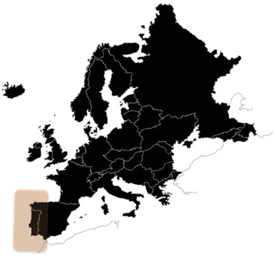
Figure 1.
Location of the Western Iberia Coast (WIC).
Although the whole region is characterized by a great primary productivity [43], it is in the northern section of the WIC that the concentrations of nutrients are assumed to be the highest. The Rias Bajas and the area of Cape Finisterre are rich in nutrients due to the high influence of the summer upwelling in this area [44]. The main oceanographic feature of the WI region is the upwelling-favorable northerly winds that prevail from April to September. The WIC comprises the northern boundary of the Eastern North Atlantic Upwelling System, which is associated with the Canary Current. The cold and nutrient-rich Eastern North Atlantic Central Water (ENACW) is promoted on to the shelf during the spring–summer upwelling, enhancing the primary production along the coast [45,46].
Although downwelling-favorable southerly winds predominate during the winter months, occasional upwelling events have also been observed during this period [47,48]. These winter events can bring water from the Iberian Poleward Current (IPC) that is more saline and warm, and less nutrient-rich, into the rias. Thus, the concentration of Chl a during the autumn–winter months could be influenced not only by upwelling events, but also by other factors such as the input of nutrients from river discharges [44]. Adding to the complexity of these oceanographic features, the normal circulation pattern inside the Rias Baixas can be reversed by the Minho estuarine plume, affecting the exchange between the Rias and the ocean and thus changing nutrient inputs [49].
2.2. Database
2.2.1. In Situ Dataset
The dataset used in this study comprised a compilation of in situ biological (i.e., Chl a) and environmental parameters (e.g., salinity, temperature, dissolved oxygen, dissolved inorganic nitrogen, phosphate, and silicate concentrations) parameters for coastal waters of the sub-typology NEA1/26e (Portugal and Spain–Galicia) within the WFD (Figure 2). Sampling stations are represented in Figure 2A. All data included in this common dataset were validated in terms of quality and consistency. In general terms, a total of 2830 valid in situ data entries, covering the period from 1995 to 2014, from a total of 36 water bodies were considered in this study (Table 1). From these, 17 coastal water bodies (CWBs) were Portuguese and 19 were from Galicia (Figure 2B). Galician CWBs include exposed and more enclosed ones, which are located within the Rias. Although not covering all the CWBs, the environmental dataset has a reasonable spatial and seasonal coverage for most parameters (Figure 3).
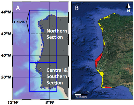
Figure 2.
Location of sampling stations (A) and coastal water bodies (CWBs) of the NEA 1/26e typology (B). CWBs highlighted in red were identified as having insufficient chlorophyll a (Chl a) data.

Table 1.
Main statistical parameters for following variables: salinity, Chl a (mg m−3), dissolved inorganic nitrogen (DIN; µM), phosphate (µM) and dissolved oxygen (DO; mg L−1). Please note the 90th, 50th, and 10th percentiles (90th %ile, 50th %ile and 10th %ile) and the standard error (SE).
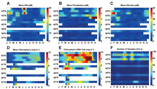
Figure 3.
Temporal and spatial (north–south) coverage of in situ data: nutrients (A) Dissolved inorganic nitrogen; (B) Phosphates; (C) Silicates and Chl a concentrations (D) Mean Chl a concentrations; (E) Chl a 90th percentile (P90). The number of Chl a samples available is also presented (F).
Focusing on the biological dataset (Chl a concentrations), significant temporal gaps were observed, especially in the Portuguese region (Figure 3D,E). From the initial 2830 data entries, only a total of 1209 entries corresponded to concomitant samples of Chl a and nitrogen, covering only 31 WBs: (i) 12 CWBs (445 data entries) in Portugal and (ii) 19 CWBs in Galicia (764 data entries). It is important to note that most data entries represented occasional sampling events, not covering the intra-annual variability. Given that most assessments of ecological/environmental quality are based on the Chl a 90th percentile (P90) metric, which is calculated for each year, it is mandatory to have sufficient samples to derive these values. Weekly or fortnightly samples would be ideal but may not be realistic due to a variety of constraints. A minimum of monthly samples during the growing season (GS) would be reasonable. The GS was already defined in the Commission Decision 2018/229 from 12 February 2018 [50] as the period from February to October. Therefore, it was essential to complement the database with additional concomitant satellite observations, as described in Section 2.2.2. This allowed the inclusion of eight additional WBs in the analysis. These eight WBs, which represent a significant percentage of the Portuguese waters, were previously identified as having insufficient Chl a data (Figure 2B). In the end, it was possible to obtain an ameliorated database covering all the 36 coastal water bodies for which it was also possible to calculate the annual Chl a P90. The final biological dataset covered the period from 1998 to 2014.
Environmental Data
Nutrient concentrations, which included dissolved inorganic nitrogen (DIN), phosphate, and silicate concentrations, were determined following the methodology described by Grasshoff et al. [51]. Most samples were analysed using a Skalar autoanalyser. Generally, temperature and salinity were measured using a multiparameter sonde, and disolved oxygen (DO) was determined following the method proposed by Winkler [52]. Occasionally, water samples were measured in the laboratory, using a salinometer. The highest nutrient concentrations were observed during winter and summer months, and especially in the northern part of the WI region (Figure 3A–C). The lowest salinities were observed in the adjacency of the most important freshwater inputs, such as river mouths. Temperatures yielded a north–south increasing gradient. DO concentrations were lower in the central and southern part of the Western Iberia region.
Phytoplankton Data (Chl a)
A comprehensive database of Chl a concentrations was compiled using existent datasets. Samples were always taken from the surface (≈0.5m depth), with Niskin bottles, and kept in dark conditions. They were filtered through a filtration slope and stored in the freezer until extraction. Most samples were measured by fluorometry. The highest concentrations were observed during spring and summer (Figure 3D,E), especially at the northern part (Galicia).
2.2.2. Satellite Dataset
In order to complement the biological dataset, the OC-CCI-v3.1 satellite chlorophyll product developed within the Ocean Colour–Climate Change Initiative (OC-CCI) project (http://esa-oceancolour-cci.org/) was selected [53]. Satellite data were downloaded from CMEMS (Iberian–Biscay–Ireland Regional Sea, available at http://marine.copernicus.eu/). This product results from merged MODIS-Aqua, SeaWIFS, and MERIS radiometric data and covers the period between 1998 and 2016. It is a ≈1 km spatial resolution daily product obtained by applying a combination of two algorithms, one for Case 2 water (OC5) [54] and the other for open ocean (OCI) [55]. Previously, Sá et al. [56] evaluated the performance of an earlier version of OC-CCI chlorophyll product using only the algorithm for open ocean [55] on images with ≈4 km spatial resolution. For Portuguese waters, they reported values of unbiased root mean square error, standard deviation, and correlation coefficient that were comparable to other products, such as MODIS OC3M chlorophyll algorithm. Nevertheless, to ensure the comparability of these satellite data, a comparison between in situ and satellite Chl a data was performed (Figure 4). Satellite points matching the in situ samples were selected considering only values for the same day and a maximum distance of 1 km. Very costal satellite data points, i.e., located at a distance of ≈2 km or less from the coast, were dismissed to minimize the complexity of accuracy issues due to the proximity to land [57,58,59]. A regional adjustment was implemented following the relationship described in Figure 4. Linear regression was observed to be significant (p < 0.05). The statistics (coefficient of determination or the square of Pearson’s correlation coefficient—r2, bias, Root Mean Square Error—RMSE, Relative Percentage Difference—RPD and Absolute Percentage Difference—APD) of the relationship are presented in Table 2. For more details on the statistics, please see Sá et al. [56] and publications cited therein.
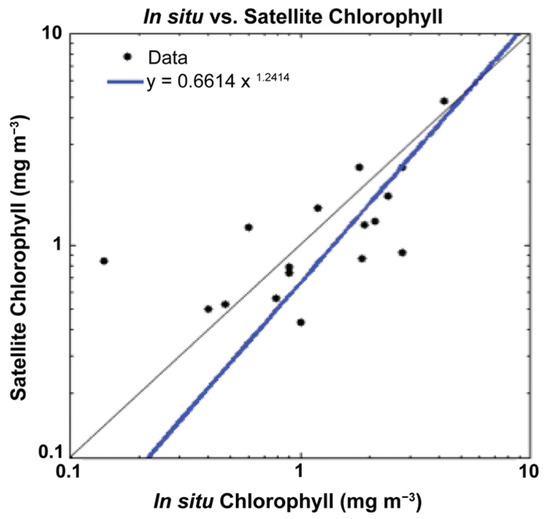
Figure 4.
Comparison between in situ Chl a and satellite Ocean Colour–Climate Change Initiative (OC-CCI) Chl a product for the common match-ups.
Table 2.
Main statistics of the comparison between in situ and satellite Chl a products for selected match-ups obtained from the same day and a maximum distance of 1 km.
2.3. Anthropogenic Pressure–LUSI Index
In order to evaluate the anthropogenic pressures, with continental origin, that are affecting the coastal waters in the WI region, the Land Uses Simplified Index [34,35,60] was applied. This index reunites the specific pressures that influence a water body and that are related to the urban, industrial, agricultural, or river characteristics that could influence phytoplankton growth. Flo et al. [34] originally defined two or three categories for each pressure and specified a score for each category. The index was obtained after the sum of all the scores, and the correction of the result with a coefficient, a correction factor related to coastline morphology, and the degree of confinement of the water body [35,61]. LUSI has no units, and in its original version [34], it may vary between 0.75 in the best scenario and 8.75 in the worst. In the present work, LUSI was adapted to the dataset, and a specific version for the west Iberian Peninsula coastal waters was created, as seen in the study of Romero et al. [61].
LUSI = (score urban + score agricultural + score typology) × correction
All the information regarding land use in the Galician coast was retrieved from the Plan Hidrolóxico da Demarcación Hidrográfica de Galicia-Costa 2015–2021. Information about Portuguese land use was compiled from Planos de Gestão de Região Hidrográfica 2016–2021, available at http://www.apambiente.pt (geovisualization available at http://sniamb.apambiente.pt/). Data about population living on the coastal municipalities of Galicia and Portugal were retrieved from the Spanish Instituto Nacional de Estadística y Censos and the Censos Report 2011 available at the Portuguese Instituto Nacional de Estatística (INE).
To obtain the scores corresponding to the urban and agricultural pressures, only the population and the utilized agricultural area (UAA) in the municipalities within a band of 10 km from the coast were utilized. Among them, the most populated coastal municipalities are Vigo and Coruña, in Galicia, and Lisbon, Sintra and Vila Nova de Gaia in Portugal. Approximately ≈54% of the Portuguese population and ≈60% of the Galician population live near the coast. In terms of land use, ≈32% of the utilized agricultural area (UAA) in Galicia and ≈50% of the UAA in Portugal are located near the coast, i.e., within a band of 10 km.
Two equations (Equations (2) and (3)) were used instead of the categories seen in Flo et al. [34]. A score of zero was attributed to a population of zero and a UAA of zero, while the maximum score of 3 was given to the largest population and largest UAA of all considered. The populations and UAA in between the zero and the maximum were given scores using the linear regression between those two points (Equations (2) and (3)):
Score urban = 2.308 × 10⁻⁶ × population number
Score agricultural = 1.264 × 10⁻⁹ × UAA (m2).
The influence of a river on the coastal waters is reflected on the salinity, or the fresh water content, being lower when the influence of the river is high. Again, instead of the three categories used in Flo et al. [34], a third equation was defined to score this pressure. For this, the mean salinity of each water body was calculated, and a score of 3 and 1 was attributed to the lowest and the highest mean salinity, respectively. The linear equation (Equation (4)) between the two points was used to assign a score to all other salinities.
Typology score = 13.503−0.345 × salinity
The sum of all the scores is multiplied by a correction number, with the objective of reflecting the continental influence that is maximized in closed areas or diminished in convex areas. Therefore, the correction number is attributed to the water bodies depending on the shape of the land (concave = 1.25, convex = 0.75, straight = 1). Industrial or other significant pressures, as harbors or channels, were not included in this index.
2.4. TRIX Trophic Index
The trophic index (TRIX), proposed by Vollenweider et al. [33], synthesizes Chl a, oxygen saturation, nitrogen, and phosphorus concentration data, in a single value. This index, which is applicable to coastal marine waters from oligotrophic to eutrophic conditions, indicates how close the state of the system is in relation to its natural conditions. It also allows monitoring the trophic condition of a given region over time and comparing the trophic situation of different, yet comparable, coastal marine waters. It is recommended that the TRIX is scaled using data from the water body under study and that only indices calculated in the same basis are comparable [33]. TRIX combines these variables as follows:
In this index, k is the number of degrees, scaling the result between 1 and 10, or 0 and 1, for example; n is the number of variables that are integrated; Mi is the measured value of the variable i; Ui is the upper limit of the variable; and Li is the lower limit of the variable. In the present work, the index was based on four state variables (n = 4), namely Chl a concentration, oxygen as the absolute deviation from saturation (abs|100−%0| = aD%0), dissolved inorganic nitrogen (DIN), and dissolved inorganic phosphorus (DIP). The chosen scaling factor was k = 10, so four trophic states could be differentiated: values below 4 indicate high quality and low trophic level, values between 4–5 mean good state and mean trophic level, 5–6 correspond to moderate state and high trophic level, and above 6 mean the state is poor and the waters are highly productive [33,62].
2.5. Assessment of Ecological Quality
Under the scope of the Water Framework Directive (WFD), the good ecological quality of coastal water bodies needs to be ensured, using chemical and biological elements, as phytoplankton. CWs of the typology NEA 1/26e are organized in four sub-typologies that include exposed and sheltered areas that are influenced by more or less intense upwelling events. These waters are fully mixed; they have depths lower than 30 m and salinities higher than 30 (Commission Decision 2018/229 from 12 February 2018) [50]. The separation between the two Portuguese sub-typologies is located at Cape Carvoeiro, as already described in Brito et al. [30], also serving to separate the Northern (which includes Galicia) and the Central and Southern Sections in this study (Figure 2). The operational methodology developed for NEA 1/26e has only one metric intercalibrated at the EU level: the Chl a P90 [29]. The current boundary conditions in action are presented in Table 3.
Table 3.
High/Good and Good/Moderate boundary conditions, in terms of Chl a P90 (mg m−3) for the four sub-typologies of the NEA 1/26e region.
2.6. Statistical Analyses
Statistical test and numerical analyses were carried out using STATISTICA 10. Regression analyses were used to evaluate the relationship between phytoplankton biomass (as Chl a P90) and pressure indicators, such as winter nutrient concentrations and the Land Uses Simplified Index (LUSI). Log transformations were implemented when data were found not to be normally distributed such as the case of Chl a concentrations. Correlations were also performed to evaluate relationships between the trophic state of coastal waters (TRIX index) and different types of pressures (LUSI: Utilized Agricultural Area, Urban, and Typology scores), in the northern, and the central and southern sections. A Principal Component Analysis (PCA) was performed to help understand possible relationships between the location of the water bodies and the trophic state of coastal waters (TRIX index) and different types of pressures (LUSI: Utilized Agricultural Area, Urban and Typology scores). The PCA was applied to a matrix of 4 variables (TRIX index, LUSI: Utilized Agricultural Area, Urban, and Typology scores) and included all the water bodies considered in this study, which were located in Portugal and Galicia. The software used was NTSYS PC (Numerical Taxonomy and Multivariate System Analysis) Version 2.0 software package (Exeter Software, New York, NY, USA).
3. Results
3.1. Chl a Variability in the Western Iberia Coast (WIC)
Phytoplankton Chl a has well-defined patterns of spatial and temporal variation in the Western Iberia (WI) region (Figure 5). From satellite observations, it is possible to identify the coastal zone as the most productive area, i.e., where the highest Chl a concentrations occur (Figure 5A). Using Chl a climatologies, it is also possible to identify the latitudinal band of 37–37.5° N as the least productive of the whole area. In the WI region, the highest climatological Chl a P90 concentrations, up to 4 mg m−3, were observed between Aveiro (≈40.7° N) and Porto (≈41.2° N). These results are in line with what is described in Table 1 for the in situ dataset. On the other hand, the offshore spring bloom, which develops from February to May, dominates the seasonal signal in the region of interest (Figure 5B,C). In general terms, it seems that the bloom ends earlier (March) in the southern sections and that it is more persistent, from February to May, in the northern sections (Figure 5B and Figure 6). Moreover, Figure 5B also highlights the importance of summer production, especially in the northern section, from July to September–October. This is also in agreement with the in situ dataset (Figure 3). The highest annual in situ Chl a P90 (15.25 mg m−3) was observed in Galicia for the year 2011. It was associated with a maximum Chl a concentration of 17.64 mg m−3 reported in October. In the southern section, although it is difficult to extract information, due to the complexity of the area integrated in the latitudes of ≈37° N, it seems that summer production is also earlier, around July (Figure 5B).
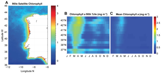
Figure 5.
Satellite Chl a P90 annual climatology (A) at the Western Iberia region, from CCI data products (1998–2016; mg m−3); seasonal and latitudinal (0.5° resolution) variation of chlorophyll a P90 (B); mg m−3 and mean concentrations (C) mg m−3. Please note that in plots B and C, each observation represents the result of integrating all data points, within each 0.5° N latitudinal band, at a given time.
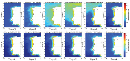
Figure 6.
Satellite Chl a P90 monthly climatologies at the Western Iberia region, from CCI data products (1998–2016; mg m−3).
3.2. Assessing Anthropogenic Pressure
3.2.1. Winter Nutrient Concentrations
The highest concentrations of winter nutrients (nitrogen, phosphates, and silicates) were always observed in the northern section, especially in Galicia (Figure 3 and Figure 7). Although there were occasional observations of very high DIN concentrations during the winter (e.g., DIN concentration of ≈300 µM reported for Galicia, in February 2012; Table 1), the P90 of the WI region during winter was of 23.71 µM (Table 1). In the Portuguese coast, the highest winter DIN concentrations (≈25.85 µM) were observed in the area between Aveiro and Porto (Figure 7B). However, it is worthwhile noting that high concentrations of DIN were also observed in the WI region during summer, up to 37.04 µM in the Aveiro-Porto area in September 2004, and up to 100 µM in Ria da Coruña in July 2012. These high summer concentrations are likely to be associated with upwelling events.
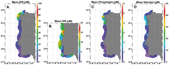
Figure 7.
In situ mean winter nutrient concentrations (µM): (A) Dissolved inorganic nitrogen at the Western Iberia (WI) region; (B) Dissolved inorganic nitrogen at the Portuguese area; (C) Phosphates at the WI region; (D) Silicates at the WI region. Please note the different scales.
The distribution of phosphates and silicates concentrations yields a similar spatial pattern to what was presented for nitrogen (Figure 7C,D), with the highest concentrations (56.60 µM for phosphates and 248.76 µM for silicates) observed in the northern section, especially in Galicia. Generally, silicate concentrations were higher during the winter period (Figure 3C). In Galicia, phosphate concentrations were relatively high (2–3 µM) throughout the whole year period.
3.2.2. LUSI Index
The LUSI index provides a semi-quantitative assessment of continental pressures on coastal waters. In its original version, the LUSI index may vary from 0.75 to 8.75. In this study, LUSI varied from 0.99 in Galicia to 5.76 in the water body in front of Tagus estuary (Figure 8). The results of this land-use based index seem to indicate a higher continental pressure in the Portuguese CWBs in comparison with waters in Galicia. The pressure categories that contributed the most for the LUSI values were the Utilized Agricultural Area (UAA) and the Typology, which is related to the freshwater influence in the coastal water body (Table 4). The highest Agriculture score of 2.87 was obtained for the CWB in front of the Sado estuary (Portuguese waters). In general terms, relatively low values of the agriculture score were obtained in Galicia. The CWB with the highest score for typology was the one in front of Douro river (Portuguese waters). Urban pressure seems much higher in Portugal than in Galicia. The highest urban score was obtained in the CWB in front of Lisbon.
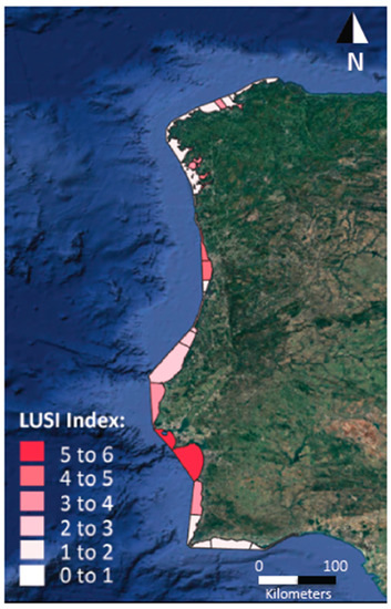
Figure 8.
LUSI index values for the different coastal water bodies. Light red represent low LUSI values and dark red represent high LUSI values. Please note the colorbar.
Table 4.
Regional values of population (×106 inhabitants) and Utilized Agricultural Area (UAA; ×108 m2). Salinity and dissolved oxygen (DO; mg L−1) are presented as regional averages. Urban, Agriculture, and Typology scores, as well as the final Land-Uses Simplified Index (LUSI) index, are also presented as regional averages. The number (N) of Water Bodies (WBs) considered in each region is provided. Please note that figures provided for population and UAA refer to land located <10 km from the coast.
3.3. TRIX Trophic Index
As described above, the trophic index (TRIX) integrates information from four concomitant variables: Chl a, deviation from oxygen saturation, nitrogen, and phosphates. These variables carry information on the anthropogenic pressures, as well as on the primary (phytoplankton growth) and secondary symptoms (oxygen reduction) of eutrophication. In terms of nutrients, the highest concentrations were observed in Galicia. In terms of phytoplankton, the highest concentrations of mean Chl a were observed in the area between Aveiro and Porto, as well as in some station in the southern section (Figure 9A). The lowest 10th percentile of oxygen (≈6 mg L−1) was mainly reported in the central section (Figure 9B). The trophic index varied from 2.86 to 6.79, with an average of 5.07. Considering values from all available years, the highest mean TRIX of 5.65 was obtained for the CWBs near the Tagus estuary (Figure 9C). High values (above 5) were also obtained for waters in Galicia, as well as between Aveiro and Porto (Figure 9C). The rest of the area yielded TRIX values below 5.
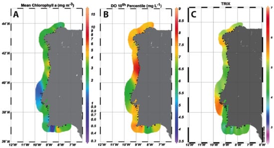
Figure 9.
(A) Mean Chl a (mg m−3); (B) Dissolved oxygen (DO) 10th %ile (mg L−1); (C) Trophic index values.
3.4. Relationship between LUSI and TRIX
Correlations performed to help better understand the contribution of the Agricultural, Urban, and Urban pressures (LUSI: Utilized Agricultural Area, Urban and Typology scores) to the trophic state of coastal waters (TRIX index) showed significant relationships between the LUSI typological score and TRIX (R = 0.63, p-value < 0.05), but not with LUSI Urban and Agricultural scores. Looking in detail at the northern section, a significant correlation (R = 0.51, p-value < 0.01) was found only with the Typology score. For the central and southern sections, positive correlations were observed with Urban (R = 0.46, p-value < 0.05) and Typology (R = 0.50, p-value < 0.05) scores, whereas a negative relationship was detected with the Agricultural score (R = −0.49, p-value < 0.05).
A PCA was performed to highlight relationships between the location of the water bodies and the trophic state of coastal waters (TRIX index), as well as different types of pressures (LUSI: Utilized Agricultural Area, Urban and Typology scores; Figure 10). The PC1 explained 51% of the variance and evidently separated water bodies more open to the ocean from those that are more enclosed due to a combination of TRIX and LUSI typology score. Coastal, but more enclosed water bodies were grouped and projected on the opposite side to the open water bodies and linked to higher values of the TRIX and LUSI typology score. This was done for all WBs, from Galicia to Southern Portugal. This pointed to a higher freshwater influence, with higher nutrient levels and primary (phytoplankton growth) and secondary symptoms (oxygen reduction) of eutrophication in these more enclosed coastal water bodies, as one would expect. The PCA also showed decoupling between some Portuguese water bodies, which are identified in Figure 10, and the rest of the surveyed areas. These Portuguese water bodies were projected close to the LUSI Utilized Agricultural and Urban scores on the PC2 axis (29%), with samples collected in front of the Tagus and Douro estuaries and the Lima to Douro coastal area more linked to higher LUSI urban score, and samples collected in front of the Sado, Mira, and Arade estuaries associated with higher LUSI Utilized Agricultural score. Interestingly, Sagres, which is considered a major upwelling center, was also observed to be associated with a higher LUSI Utilized Agriculture score. Contrastingly, the other water bodies, either more enclosed or open to the ocean, were gathered in the opposite side to the above-mentioned Portuguese water bodies, which emphasizes that those areas are less influenced by agriculture activities and close to less impacting urban areas.
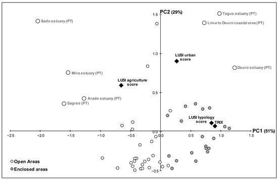
Figure 10.
Projection of trophic state of coastal waters (TRIX index) and LUSI Utilized Agricultural Area, Urban, and Typology score values, and assessed water bodies, obtained from Principal Component Analysis (PCA). Percentage of total variance is indicated in brackets close to principal component axes. Please note that all labels for the estuary refer to coastal sampling stations located in front of the estuarine mouths.
3.5. Use of Pressure Indicators to Understand Eutrophication
To understand the eutrophication process and to execute management actions, it is mandatory to link the pressures and the responses directly. This is also required to comply with the EU Directives, such as the Water Framework Directive (WFD). In order to achieve this, and due to the existence of different oceanographic processes, two main areas were considered: northern (including Galicia) vs. central and southern sections (Figure 11), as already described in Section 2.5. The main reason behind this separation is the existence of strong and persistent upwelling in the northern section. Moreover, these areas consist of two already established sub-typologies of the NEA 1/26E, under the WFD.
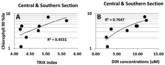
Figure 11.
(A) Relationship between Chl a P90 (mg m−3) and TRIX index in the central and southern section (i.e., in the upwelling sub-typology); (B) Relationship between Chl a P90 (mg m−3) and dissolved inorganic nitrogen (DIN; µM) concentrations, also in the central and southern section.
3.5.1. Phytoplankton Response to Dissolved Nutrients
No significant relationship was observed in the northern section (p-value > 0.05). However, a significant relationship was found between Chl a P90 and winter nitrogen concentrations (Figure 11B; p-value < 0.05; R2 = 0.76). The highest Chl a P90 was of 8.11 mg m−3, which corresponded to a nitrogen concentration of 11.67 µM.
3.5.2. Relationship between Phytoplankton and LUSI
A significant correlation between LUSI and Chl a was observed for Galician offshore waters (R = 0.34; p-value < 0.05). However, this is considered a weak relationship due to the low correlation coefficient observed (R <0.4). No significant relationship was observed for the rest of the northern section (Portugal), as well as the central and southern section (p-value > 0.05). In the Galician offshore waters, all Chl a values were associated with a LUSI index of 2.5 or below.
3.5.3. Relationship between Phytoplankton and TRIX
A significant relationship was obtained between Chl a P90 and the trophic index (TRIX) for the central and southern sections (Figure 11A; p-value < 0.05). The highest TRIX value in the central and southern section was of 5.65, which corresponded to a Chl a P90 of 6.39 mg m−3.
3.6. Ecological Quality of Coastal Water Bodies (CWBs)
Overall, in the northern section, no CWB was classified with a “Moderate” state or worse, i.e., all WBs had Chl a P90 values below 12 mg m−3 (Portugal and Galicia-Rias) and 9 mg m−3 (Galicia offshore). Actually, most water bodies were classified with “High” status, except for seven CWBs that were classified with “Good” condition. A significant correlation was observed between Chl a P90 and LUSI, which could suggest an impact of continental anthropogenic pressures. However, LUSI values were relatively low. TRIX values higher than 5 were found in association with Chl a P90 concentrations of ≈8 mg m−3, but those index values may be strongly affected by the high concentrations of nutrients observed during the summer. No apparent problems on oxygen reduction were observed (Figure 9B).
In the southern section, all CWBs were classified with “High” condition, except two classified with “Good” condition, which are located at the adjacency of two major rivers: Tagus and Guadiana. Most WBs were characterized by winter nitrogen concentrations of 10 µM or below (and TRIX below 5; Figure 11), except for the two located near the Tagus and Guadiana with concentrations of approximately 12 µM (and TRIX higher than 5). It is worth noting that Sagres, an area without inputs from rivers and weak continental pressure (LUSI of 1.74), apparently had natural winter DIN concentrations of 10 µM. Although relatively high (≈6 mg L−1), the lowest concentrations of dissolved oxygen were also observed in the CWBs in front of the rivers Tagus and Guadiana (Figure 9B).
4. Discussion
4.1. Eutrophication Indicators for Coastal Waters in the WIC
Past experience has shown difficulties in the integration of the natural spatial and temporal variability of phytoplankton Chl a, especially in coastal and transitional waters of the WIC [8,30]. These waters are strongly influenced by seasonality as well as by the complexity of processes taking place in the land–sea interface, such as river discharges, run-off, and upwelling, making it difficult to discriminate the natural signals from those triggered by human action [63]. In this regard, it is essential to understand the phytoplankton natural variation in coastal waters, as it constitutes the baseline or the starting point against which the anthropogenic pressures should be evaluated. Given the limited number of coastal in situ phytoplankton samples and the limited spatial and temporal coverage of such samples, it is crucial to use cost-effective methods that are able to provide the temporal and spatial coverage required. Ocean Color Remote Sensing (OCRS) techniques offer the opportunity to comply with these requirements and to characterize the background signal that is likely to be driven by seasonality and natural spatial gradients (e.g., coast–ocean and north–south) and processes. In this context, Gohin et al. [64] used 20 years of satellite and in situ observations to evaluate changes in the water quality in the English Channel and the northern Bay of Biscay. Satellite data allowed increasing the frequency of spatial observations. Moreover, the recently developed Northwest Pacific Action Plan (NOWPAP) Eutrophication Assessment Tool (NEAT), based on satellite data, is another example of simple, robust, and effective satellite observation techniques to detect potential eutrophic zones based on Chl a levels and trends [65]. The analysis of OC-CCI data for the WIC region provided confirmation that growing season starts in February, with the development of an offshore spring bloom, reaching average concentrations from 2 to 4 mg m−3 for the Chl a P90. The growing season continues until the end of October, with high phytoplankton biomass (average Chl a concentrations > 5 mg m−3) near the coast during the upwelling season. This study sets the background knowledge and Chl a levels for the future implementation of operational monitoring based on the use of satellite Chl a.
4.2. Phytoplankton Response to Anthropogenic Pressures
The main rationale behind the EU WFD and MSFD is that anthropogenic pressure is likely to cause a deviation from the natural state, i.e., from reference conditions. Reference conditions are clearly one of the most complex points of their implementation, as it is almost virtually impossible to find such reference conditions for most water bodies. Working with pressure gradients instead of relying only on the most pristine conditions is seen as a practical way to evaluate the degree of impacts. However, in order to follow this route, it is essential to have appropriate, i.e., high quality, information on anthropogenic pressure.
Pressure indicators based on measured parameters, such as nutrients, have to rely on the snapshot taken at the time of sampling. In fact, some level of mismatch between pressure and impact is likely to occur, given that phytoplankton requires nutrients to grow and cells may take some time (hours to days) to increase their numbers [66,67]. Apart from this, other factors, such as high turbidity, may contribute toward the absence of a positive correlation between the pressure and the biological indicator [68,69].
In this case, results indicate that this study was successful in reporting a significant positive relationship between Chl a P90 and DIN concentration, which is used as an index of anthropogenic action, for CWs at the central and southern sections of the Western Iberia Coast (WIC). A positive response of Chl a to increased nitrogen has already been reported at the vicinity of major rivers in the WIC, such as Douro and Guadalquivir [63]. However, no significant relationship was observed in the northern part of the WIC. A land-use-based pressure indicator, such as LUSI, may represent a more reliable and stable option, as it should reflect the long-term human pressure on the coastal zone [35]. LUSI has already been successfully applied to a variety of coastal and enclosed waters in Europe [61,70]. However, in this case, only a weak but significant correlation between the biological metric, i.e., Chl a P90, and the LUSI index was observed at Galicia, where relatively low LUSI values were found. These low LUSI values observed on the Galician coastal area indicate the absence or only a slight influence of continental pressures, especially in terms of the utilized agricultural area (UAA) in the municipalities within a band of 10 km from the coast. High LUSI values indicate that continental pressures strongly influence coastal waters [60], which seems to be the case of the water bodies in front of the Tagus estuary. The apparent link between high LUSI values and the existence of large estuaries highlights the need to adjust and optimize the LUSI methodology, in the context of the WIC, so that it is able to better differentiate the anthropogenic effect from natural variability. However, it is important to keep in mind that this outcome may also be the result of using a limited dataset. Further efforts should be done in the future to overcome these gaps.
4.3. Trophic Level and Ecological Quality Status (EQS)
The LUSI-associated scores allowed to differentiate between the urban, agricultural, and freshwater influence impacts that might be associated with the TRIX values obtained. None of the TRIX values were higher than 6, which is the threshold for degraded water quality and very high trophic levels [33,62]. This is in line with what has been previously reported by MAMAOT [71] and Cabrita et al. [8]. More enclosed water bodies were linked to higher values of the TRIX and LUSI typology score, denoting higher freshwater influence, with higher nutrient levels and primary and secondary symptoms of eutrophication. The highest TRIX values were observed in the central area, near Lisbon Bay. These were the stations where the lowest DO levels were recorded and the highest nitrogen concentrations were observed. In the central and southern sections, all water bodies classified in an intermediate level of water quality, according to TRIX, had concentrations of Chl a P90 from ≈6 to 8.5 mg m−3, which corresponded to nitrogen concentrations higher than 10 µM. The relatively high TRIX values, linked to relatively high LUSI urban score, concomitantly obtained for the water body in front of Tagus estuary suggest that this area near the Lisbon bay may be considered as a problem area following the OSPAR (Convention for the Protection of the Marine Environment of the North-East Atlantic) classification or as an area of ongoing concern that should be subject to continued monitoring. Other Portuguese water bodies, such as the Douro estuary and the Lima to Douro coastal area, also showed high LUSI urban score, and the Sado, Mira, and Arade estuaries and Sagres were areas where agricultural activities had high impact (high LUSI Utilized Agricultural score), which suggests that monitoring should be maintained in these areas to follow the evolution of their trophic level and EQS. Contrastingly, the other water bodies, either more enclosed or open to the ocean, appeared as less influenced by agriculture activities and located close to less impacting urban areas.
Overall, these results seem to confirm the boundary values for the NEA 1/26e sub-typology “Portugal-upwelling” that resulted from the last intercalibration exercise and are published in the Commission Decision 2018/229 from 12 February 2018 [50].
In the northern section, none of the water bodies were considered in a degraded state, i.e., with TRIX values higher than 6. In fact, TRIX values varied between 4.4 and 5.7, and these are associated with LUSI typology scores fluctuating between 1.2 and 3.0. Most water bodies had relatively high concentrations of nitrogen and phosphate, up to 70 µM and 4 µM (average winter concentrations), respectively, and a wide range of Chl a P90 concentrations, from ≈2.3 to 9 mg m−3. Interestingly, one of the highest concentrations of Chl a P90 (≈8 mg m−3), on average, was associated with the lowest TRIX value in the northern section (≈4.4), which seem to indicate that high phytoplankton production may occur naturally in these waters that are considered in good quality state. This may be promoted by natural nutrient enrichment, given that this region is characterized by strong and persistent upwelling periods, especially in the summer [43,63].
4.4. Future Advances for Operational Monitoring
For operational monitoring of marine eutrophication, additional OCRS products with higher spatial resolution could be selected. It is the case of the Sentinel missions. The Ocean and Land Color Instrument (OLCI) on board Sentinel-3 is now providing high-quality Chl a products with 300 m spatial resolution. In addition, the MultiSpectral Instrument (MSI) on board Sentinel-2 is able to provide 10, 20, and 60 m spatial resolution data. Although several studies have reported problems in the atmospheric correction part of the processor [72], it is worth assessing the accuracy of these products, even if extensive training of the Chl a algorithm is required [73]. An important constraint associated with the use of OCRS products is the possible overestimation of Chl a concentrations in coastal waters where terrestrial substances (such as iron-rich minerals and humus) contribute significantly to the total light absorption and scattering in water but do not co-vary with phytoplankton [74].
The future NASA’s Plankton, Aerosol, Cloud and ocean Ecosystem (PACE) mission will also be of interest for the further development of eutrophication indicators. Although with a 1 km spatial resolution, it will have an improved spectral resolution of 5 nm, from the ultraviolet to the near infrared. This will allow the development of methods to discriminate spectral signatures and provide data on specific phytoplankton groups, such as phytoplankton functional types [75,76], thus integrating the community structure in the analysis.
To fully comply with the WFD, changes in bloom frequency and community structure should be assessed [77], and satellite data have all the potential to provide the appropriate datasets. Recently, Papathanasopoulou et al. [78] highlighted the importance of organizing expert working groups to produce harmonized satellite observation methods across countries with well-characterized uncertainties. Harmonized products can effectively resolve transboundary issues in terms of water quality assessments. For the WFD context, these satellite products should be comparable with in situ nationally approved and intercalibrated methods. Furthermore, high spectral resolution data should also promote monitoring at the species level, enabling early warning and harmful algal bloom follow-up [79]. Therefore, such methodologies are likely to contribute toward an operational biodiversity monitoring and to further testing eutrophication indicators (e.g., species shift in floristic composition and toxic algal blooms).
5. Conclusions
This study contributes to the understanding of the temporal and spatial variability of eutrophication indicators at the Western Iberia Coast. A clear pressure–response relationship between Chl a and pressure indicators (nitrogen concentrations, TRIX and LUSI) was observed in these coastal waters, highlighting the relevance of integrating phytoplankton in quality assessments. The most problematic areas, i.e., the ones with ongoing concern and potentially high eutrophication susceptibility, were identified as located at the vicinity of important estuaries (e.g., Douro and Tagus), where continuous monitoring should be performed. The use of ocean color remote sensing was crucial to include all coastal WBs in the analysis, elevating the number of concomitant (Chl a and environment) data entries. The OC-CCI database, composed of 20 years worth of data, also allowed expanding the spatial and temporal coverage of this work, setting the background Chl a levels for the implementation of operational monitoring based on the use of satellite Chl a. However, this is not the standard procedure for WFD reporting yet. The use of satellite data products in the context of the WFD would benefit from formal acknowledgement at the European and national levels, which could be done by updating the WFD-associated documentation. In the future, operational monitoring of eutrophication indicators should be further improved in order to provide (i) products with high spatial resolution; (ii) coastal Chl a products with lower uncertainties; (iii) harmonized satellite products and WFD metrics across countries; and (iv) metrics that provide information on phytoplankton phenology and community composition.
Author Contributions
Conceptualization: A.C.B.; methodology: A.C.B., P.G.-A., C.G., M.T.C.; writing—original draft preparation: A.C.B., P.G.-A., M.T.C.; writing—review and editing: A.C.B., C.G., M.N., M.T.M., M.T.C. All authors have read and agreed to the published version of the manuscript.
Funding
Ana C. Brito and Paloma Garrido-Amador were funded by Fundação para a Ciência e a Tecnologia (FCT) Investigador Programme (IF/00331/2013). Ana C. Brito was also funded by Fundação para a Ciência e a Tecnologia (FCT) Scientific Employment Stimulus (CEECIND/00095/2017) Programme. Maria Teresa Cabrita wishes to acknowledge individual grant (SFRH/BPD/50348/2009) by FCT and M.T. Moita wants to thank the FCT support by UIDB/04326/2020. This study received support from the Infrastructure CoastNet (PINFRA/22128/2016), funded by FCT and the Regional Development Fund (FEDER), through LISBOA2020 and ALENTEJO2020 regional operational programmes, in the framework of the National Roadmap of Research Infrastructures of strategic relevance. It also received further support from EU H2020 CERTO Project (LC-SPACE-04-EO-2019-2020; Grant agreement nº 870349) and Fundação para a Ciência e a Tecnologia, through the strategic project (UID/MAR/04292/2020) granted to MARE.
Acknowledgments
The authors are grateful to Augas de Galicia and Laboratorio de Medio Ambiente de Galicia, Dirección Xeral de Calidade Ambiental e Cambio Climático, Xunta de Galicia for kindly providing information on biological (chlorophyll a) and environmental parameters that were essential for this publication. We would also like to thank the Subdirectora Xeral de Meteoroloxía e Cambio Climático, Maria Luz Macho Eiras, and Alberto Gayoso for supporting this study. The authors also acknowledge the constant support of Susana Nunes, from Agência Portuguesa do Ambiente (APA).
Conflicts of Interest
The authors declare no conflict of interest.
References
- Stachowicz, J.J.; Whitlatch, R.B.; Osman, R.W. Species diversity and invation resistance in marine ecosystem. Science 1999, 286, 1577–1579. [Google Scholar] [CrossRef]
- Snelgrove, P.; Berghe, E.V.; Miloslavich, P.; Archambault, P.; Bailly, N.; Brandt, A.; Bucklin, A.; Clark, M.; Dahdouh-Guebas, F.; Halpin, P.; et al. Global patterns in Marine Biodiversity. In First Global Integrated Marine Assessment (First World Ocean Assessment); UN General Assembly; United Nations: New York, NY, USA, 2016; Chapter 34; p. 37. [Google Scholar]
- EUROSTAT. Available online: https://ec.europa.eu/eurostat/statistics-explained/index.php/Archive:Coastal_regions_-_population_statistics (accessed on 11 April 2018).
- Socolow, R.H. Nitrogen management and the future of food: Lessons from the management of energy and carbon. Proc. Natl. Acad. Sci. USA 1999, 96, 6001–6008. [Google Scholar] [CrossRef]
- Neumann, B.; Vafeidis, A.T.; Zimmermann, J.; Nicholls, R.J. Future coastal population growth and exposure to sea-level rise and coastal flooding- a global assessment. PLoS ONE 2015, 10, e0118571. [Google Scholar] [CrossRef] [PubMed]
- Anderson, J.H.; Conley, D.J. Eutrophication in coastal marine ecosystems: Towards better understanding and management strategies. Hydrobiologia 2009, 629, 1–4. [Google Scholar] [CrossRef]
- Le Moal, M.; Gascuel-Odoux, C.; Ménesguen, A.; Souchon, Y.; Étrillard, C.; Levain, A.; Moatar, F.; Pannard, A.; Souchu, P.; Lefebvre, A.; et al. Eutrophication: A new wine in an old bottle? Sci. Total Environ. 2019, 651, 1–11. [Google Scholar] [CrossRef]
- Cabrita, M.T.; Silva, A.; Oliveira, P.; Angélico, M.M.; Nogueira, M. Assessing eutrophication in the Portuguese continental exclusive economic zone within the European Marine Strategy Framework Directive. Ecol. Indic. 2015, 58, 286–299. [Google Scholar] [CrossRef]
- Norring, N.P.; Jorgensen, E. Eutrophication and agroculture in Denmark: 20 years of experience and prospects for the future. Hydrobiologia 2009, 629, 65–70. [Google Scholar] [CrossRef]
- Petersen, J.D.; Rask, N.; Madsen, H.B.; Jorgensen, O.T.; Petersen, S.E.; Nielsen, S.V.K.; Pedersen, C.B.; Jensen, M.H. Odense Pilot River Basin: Implementation of the EU Water Framework Directive in a shallow eutrophic estuary (Odense Fjord, Denmark) and its upstream catchment. Hydrobiologia 2009, 629, 71–89. [Google Scholar] [CrossRef]
- Conley, D.J.; Humborg, C.; Rahm, L.; Savchuk, O.P.; Wulff, F. Hypoxia in the Baltic Sea and basin-scale changes in phosphorus biogeochemistry. Environ. Sci. Technol. 2002, 36, 5315–5320. [Google Scholar] [CrossRef]
- Borja, A.; Dauer, D.; Elliott, M.; Simenstad, C. Medium- and Long-term Recovery of Estuarine and Coastal Ecosystems: Patterns, Rates and Restoration Effectiveness. Estuaries Coast 2010, 33, 1249–1260. [Google Scholar] [CrossRef]
- Boesch, D.F. Barriers and Bridges in Abating Coastal Eutrophication. Front. Mar. Sci. 2019, 6, 123. [Google Scholar] [CrossRef]
- Paerl, H.W.; Valdes, L.; Pinckney, J.; Piehler, M.; Dyble, J.; Moisander, P. Phytoplankton photopigments as indicators of estuarine and coastal eutrophication. BioScience 1997, 53, 953–964. [Google Scholar] [CrossRef]
- Paerl, H.W.; Dennis, R.L.; Whitall, D.R. Atmospheric Deposition of Nitrogen: Implication for nutrient over-enrichment of coastal waters. Estuaries 2002, 25, 677–693. [Google Scholar] [CrossRef]
- Zheng, T.; Cao, H.; Xy, J.; Yan, Y.; Lin, X.; Huang, J. Characteristics of Atmospheric Deposition during the period of algal bloom formation in urban water bodies. Sustainability 2019, 11, 1703. [Google Scholar] [CrossRef]
- Sinha, E.; Michalak, A.M.; Balaji, V. Eutrophication will increase during the 21st century as a result of precipitation changes. Science 2017, 357, 405–408. [Google Scholar] [CrossRef]
- Najjar, R.G.; Walker, P.J.; Andersen, E.J.; Barron, R.J.; Bord, R.J.; Gibson, J.R.; Kennedy, V.S.; Knight, C.G.; Megonigal, J.P.; O’Connor, E.R.; et al. The potential impacts of climate change on mid-Atlantic coastal region. Clim. Res. 2000, 14, 219–233. [Google Scholar] [CrossRef]
- Cloern, J.E. Our evolving conceptual model of the coastal eutrophication problem. Mar. Ecol. Prog. Ser. 2001, 210, 223–253. [Google Scholar] [CrossRef]
- Diaz, R.; Rosenberg, R. Marine benthic hypoxia: A review of its ecological effects and behavioural response of benthoc macrofauna. Oceanogr. Mar. Biol. 2015, 33, 245–303. [Google Scholar]
- Nixon, S.W. Eutrophication and the macroscope. In Eutrophication in Coastal Ecosystems. Developments in Hydrobiology; Andersen, J.H., Conley, D.J., Eds.; Springer: Dordrecht, The Netherlands, 2009; Volume 207, pp. 5–19. [Google Scholar]
- Howarth, R.; Marino, R. Nitrogen as the limiting nutrient for eutrophication in coastal marine ecosystems: Evolving views over three decades. Limnol. Oceanogr. 2006, 51, 364–376. [Google Scholar] [CrossRef]
- Conley, D.J.; Castensen, J.; Vaquer-Sunyer, R.; Duarte, C.M. Ecosystem thresholds with hypoxia. In Eutrophication in Coastal Ecosystems. Developments in Hydrobiology; Andersen, J.H., Conley, D.J., Eds.; Springer: Dordrecht, The Netherlands, 2009; Volume 207, pp. 21–29. [Google Scholar]
- Duarte, C.M. Coastal eutrophication research: A new awareness. Hydrobiologia 2009, 629, 263–269. [Google Scholar] [CrossRef]
- Jaanus, A.; Toming, K.; Hallfors, S.; Kaljurand, K.; Lips, I. Potential phytoplankton indicator species for monitoring Baltic coastal waters in the summer period. In Eutrophication in Coastal Ecosystems. Developments in Hydrobiology; Andersen, J.H., Conley, D.J., Eds.; Springer: Dordrecht, The Netherlands, 2009; Volume 207, pp. 157–168. [Google Scholar]
- Devlin, M.; Best, M.; Coates, D.; Bresnan, E.; O’Boyle, S.; Park, R.; Silke, J.; Cusack, C.; Skeats, J. Establishing boundary classes for the classification of the UK marine waters using phytoplankton communities. Mar. Pollut. Bull. 2007, 55, 91–103. [Google Scholar] [CrossRef]
- Revilla, M.; Franco, J.; Bald, J.; Borja, A.Å.L.; Laza, A.; Seoane, S.; Valencia, V. Assessment of the phytoplankton ecological status in the Basque coast (northern Spain) according to the European Water Framework Directive. J. Sea Res. 2009, 61, 60–67. [Google Scholar] [CrossRef]
- Ferreira, J.G.; Andersen, J.H.; Borja, A.; Bricker, S.; Camp, J.; Silva, M.C.; Garcés, E.; Heiskanen, A.S.; Humborg, C.; Ignatiades, L.; et al. Overview of eutrophication indicators to assess environmental status within the European Marine Strategy Framework Directive. Estuar. Coast. Shelf Sci. 2011, 93, 117–131. [Google Scholar] [CrossRef]
- Salas, F.; Teixeira, H. WFD Intercalibration Data Archives: Coastal and Transitional Waters; European Commission: Brussels, Belgium, 2019; p. 91. [Google Scholar]
- Brito, A.C.; Brotas, V.; Caetano, M.; Coutinho, T.P.; Bordalo, A.; Icely, J.; Neto, J.; Serôdio, J.; Moita, T. Defining phytoplankton class boundaried in Portuguese transitional waters: An evaluation of the ecological quality status according to the Water Framework Directive. Ecol. Indic. 2012, 19, 5–14. [Google Scholar] [CrossRef]
- Birk, S.; Bonne, W.; Borja, A.; Brucet, S.; Courrat, A.; Poikane, S.; Solimini, A.; Van de Bund, W.; Zampoukas, N.; Hering, D. Three hundred ways to assess Europe’s surface waters: An almost complete overview of biological methods to implement the Water Framework Directive. Ecol. Indic. 2012, 18, 31–41. [Google Scholar] [CrossRef]
- Xu, F.L.; Tao, S.; Dawson, R.W.; Li, B.G. A GIS-based method of lake eutrophication assessment. Ecol. Model. 2001, 144, 231–244. [Google Scholar] [CrossRef]
- Vollenweider, R.; Giovanardi, F.; Montanari, G.; Rinaldi, A. Characterization of the trophic conditions of marine coastal waters with special reference to the NW Adriatic Sea: Proposal for a trophic scale, turbidity and generalized water quality index. Environmentrics 1998, 9, 329–357. [Google Scholar] [CrossRef]
- Flo, E.; Camp, J.; Garcés, E. Assessment of pressure methodology for biological quality element phytoplankton: Land Uses Simplified Index (LUSI). In Mediterranean Geographical Intercalibration Group-Coastal Waters-Biological Quality Element Phytoplankton-France and Spain; Water Framework Directive Intercalibration Phase 2: Milestone 5 report; European Commission: Brussels, Belgium, 2011; p. 32. [Google Scholar]
- Flo, E. Opening the Black Box of Coastal Inshore Waters in the NW Mediterranean Sea: Environmental Quality Tools and Assessment. Ph.D. Thesis, Universitat de Barcelona, Barcelona, Spain, November 2017. [Google Scholar]
- Vascetta, M.; Kauppila, P.; Furman, E. Aggregate indicators in coastal policy making: Potentials of the Trophic Index TRIX for sustainable considerations of eutrophication. Sustain. Dev. 2008, 16, 282–289. [Google Scholar] [CrossRef]
- Salas, F.; Teixeira, H.; Marcos, C.; Marques, J.C.; Pérez-Ruzafa, A. Applicability of the trophic index TRIX in two transitional ecosystems: The Mar Menor lagoon (Spain) and the Modengo estuary (Portugal). ICES J. Mar. Sci. 2008, 65, 1442–1448. [Google Scholar] [CrossRef]
- Carletti, A.; Heinskanen, A.S. Water Framework Directive Intercalibration Technical Report Part 3: Coastal and Transitional Waters; EUR 23838 EN/3; Publication Office of the European Union: Luxembourg, 2009. [Google Scholar]
- Saraiva, S.; Pina, P.; Martins, F.; Santos, M.; Braunschweig, F.; Neves, R. Modelling the influence of nutrient loads on Portuguese estuaries. Hydrobiologia 2007, 587, 5–18. [Google Scholar] [CrossRef]
- Brito, A.; Newton, A.; Tett, P.; Fernandes, T. Sediment-water interactions in a coastal shallow lagoon, Ria Formosa (Portugal): Implications within the Water Framework Directive. J. Environ. Monit. 2010, 12, 318–328. [Google Scholar] [CrossRef] [PubMed]
- Peliz, A.; Rosa, T.; Santos, M.; Pissarra, J. Fronts, jets, and counter-flows in the Western Iberian upwelling system. J. Mar. Syst. 2002, 35, 61–77. [Google Scholar] [CrossRef]
- Santos, M.; Peliz, A.; Dubert, J.; Oliveira, P.B.; Angélico, M.; Ré, P. Impact of a winter upwelling event on the distribution and transport of sardine (Sardina pilchardus) eggs and larvae off western Iberia: A retention mechanism. Cont. Shelf Res. 2004, 24, 149–165. [Google Scholar] [CrossRef]
- Bode, A.; Alvarez, M.; Ruíz-Villarreal, M.; Varela, M. Changes in phytoplankton production and upwelling intensity off A Coruna (NW Spain) for the last 28 years. Ocean Dyn. 2019, 69, 861–873. [Google Scholar] [CrossRef]
- Alvarez, I.; Lorenzo, M.N.; de Castro, M. Analysis of chlorophyll a concentration along the Galicias coast: Seasonal variability and trends. ICES J. Mar. Sci. 2012, 69, 728–738. [Google Scholar] [CrossRef]
- Fiuza, A. Hidrologia e Dinâmica das Águas Costeiras de Portugal (Hydrology and Dynamics of the Portuguese Coastal Waters). Ph.D. Thesis, University of Lisbon, Lisbon, Portugal, 1984. [Google Scholar]
- Álvarez-Salgado, X.A.; Gago, J.; Miguez, B.M.; Gilcoto, M.; Pérez, F. Surface waters of the NW Iberian Margin: Upwelling on the shelf versus outwelling of upwelled waters from the Rias Baixas. Estuar. Coast. Shelf Sci. 2000, 51, 821–837. [Google Scholar] [CrossRef]
- Alvarez, I.; de Castro, M.; Prego, R.; Gómez-Gesteira, M. Hydrographic characterization of a Winter-upwelling event in the Ria of Pontevedra (NW Spain). Estuar. Coast. Shelf Sci. 2003, 56, 869–876. [Google Scholar] [CrossRef]
- Alvarez, I.; Ospina-Alvarez, N.; Pazos, Y.; de Castro, M.; Bernardez, P.; Campos, M.J.; Gomez-Gesteira, J.L.; Alvarez-Ossorio, M.T.; Varela, M.; Gomez-Gesteira, M.; et al. A Winter upwelling event in the Northern Galician Rias: Frequency and oceanographic implications. Estuar. Coast. Shelf Sci. 2009, 82, 573–582. [Google Scholar] [CrossRef]
- Sousa, M.C.; Mendes, R.; Alvarez, I.; Vaz, N.; Gomez-Gesteira, M.; Dias, J.M. Unusual circulation patterns of the Rias Baixas induced by Minho Freshwater intrusion (NW of the Iberian Peninsula). PLoS ONE 2014, 9, e112587. [Google Scholar] [CrossRef]
- EC (European Commission). Commission Decision 2018/229 of 12 February 2018 establishing, pursuant to Directive 2000/60/EC of the European Parliament and of the Council, the values of the Member State monitoring system classifications as a result of the intercalibration exercise and repealing Commission Decision 2013/480/EU. Off. J. Eur. Union 2018, 47, 1–91. [Google Scholar]
- Grasshoff, K.; Ehrhardt, M.; Kremling, K. Methods of Seawater Analysis, 2nd ed.; Verlag Chemie Weinhein: New York, NY, USA, 1983; p. 419. [Google Scholar]
- Winkler, L.W. Die Bestimmung des in Wasser gelosten Sauerstoffen. Ber. Dtsch. Chem. Ges. 1888, 21, 2843–2855. [Google Scholar] [CrossRef]
- Sathyendranath, S.; Grant, M.; Brewin, R.J.W.; Brockmann, C.; Brotas, V.; Chuprin, A.; Doerfffer, R.; Dowell, M.; Farman, A.; Groom, S.; et al. ESA Ocean Colour Climate Change Initiative (Ocean_Colour_cci): Version 3.1 Data; Centre for Environmental Data Analysis: Didcot, UK, 4 July 2018. [Google Scholar]
- Gohin, F.; Saulquin, B.; Oger-Jeanneret, H.; Lozac’h, L.; Lampert, L.; Lefebvre, A.; Riou, P.; Bruchon, F. Towards a better assessment of the ecological status of coastal waters using satellite-derived chlorophyll-a concentrations. Remote Sens. Environ. 2008, 112, 3329–3340. [Google Scholar] [CrossRef]
- Hu, C.; Lee, Z.; Franz, B.A. Chlorophyll-a algorithms for oligotrophic oceans: A novel approach based on three-band reflectance difference. J. Geophys. Res. 2012, 117, C01011. [Google Scholar] [CrossRef]
- Sá, C.; D’Alimonte, D.; Brito, A.C.; Kajiyama, T.; Mendes, C.R.; Vitorino, J.; Oliveira, P.B.; da Silva, J.; Brotas, V. Validation of standard and alternative satellite ocean-color chlorophyll products off Western Iberia. Remote Sens. Environ. 2015, 168, 403–419. [Google Scholar] [CrossRef]
- Ruddick, K.G.; Ovidio, F.; Rijkeboer, M. Atmospheric correction of SeaWiFS imagery for turbid coastal and inland waters. Appl. Opt. 2000, 39, 897–912. [Google Scholar] [CrossRef]
- Bulgarelli, B.; Kiselev, V.; Zibordi, G. Adjacency effects in satellite radiometric products from coastal waters: A theoretical analysis for the northern Adriatic Sea. Appl. Opt. 2017, 56, 854–869. [Google Scholar] [CrossRef]
- Novoa, S.; Doxaran, D.; Ody, A.; Vanhellemont, Q.; Lafon, V.; Lubac, B.; Gernez, P. Atmospheric corrections and multi-conditional algorithm for multi-sensor remote sensing of suspended particulate matter in low-to-high turbidity levels coastal waters. Remote Sens. 2017, 9, 61. [Google Scholar] [CrossRef]
- Flo, E.; Garcés, E.; Camp, J. Land Uses Simplified Index (LUSI): Determining Land Pressures and their link with coastal eutrophication. Front. Mar. Sci. 2019, 6, 18. [Google Scholar] [CrossRef]
- Romero, I.; Pachés, M.; Martínez-Guijarro, R.; Ferrer, J. Glophymed: An index to establish the ecological status for the Water Framework Directive based on phytoplankton in coastal waters. Mar. Pollut. Bull. 2013, 75, 218–223. [Google Scholar] [CrossRef]
- Penna, B.; Capellacci, S.; Ricci, F. The influence of the Pro River discharge phytoplankton bloom dynamics along the coastline of Pesaro (Italy) in the Adriatic Sea. Mar. Pollut. Bull. 2004, 48, 321–326. [Google Scholar] [CrossRef]
- Ferreira, A.; Garrido-Amador, P.; Brito, A.C. Disentangling environmental drivers of phytoplankton biomass off Western Iberia. Front. Mar. Sci. 2019, 6, a44. [Google Scholar] [CrossRef]
- Gohin, F.; Zande, D.; Tilstone, G.; Eleveld, M.; Lefebvre, A.; Andrieux-Loyer, F.; Blauw, A.; Bryère, P.; Devreker, D.; Garnesson, P.; et al. Twenty years of satellite data and in-situ observations of surface chlorophyll-a from the northern Bay of Biscay to the eastern English Channel. Is the water quality improving? Remote Sens. Environ. 2019, 233, 111343. [Google Scholar] [CrossRef]
- Terauchi, G.; Maure, E.R.; Yu, Z.; Wu, Z.; Lee, C.; Kachur, V.; Ishizaka, J. Assessment of eutrophication using remotely sensed chlorophyll-a in the Northwest Pacific region. In Proceedings of the Remote Sensing of the Ocean and Coastal Ocean and Inland Waters, Honolulu, HI, USA, 24–26 September 2018; Volume 10778. [Google Scholar] [CrossRef]
- Cloern, J. The relative importance of light and nutrient limitation of phytoplankton growth: A simple indez of coastal ecosystem sensitivity to nutrient enrichment. Aquat. Ecol. 1999, 33, 3–15. [Google Scholar] [CrossRef]
- Loureiro, S.; Icely, J.; Newton, A. Enrichment experiments and primary production at Sagres (SW Portugal). J. Exp. Mar. Biol. Ecol. 2008, 359, 118–125. [Google Scholar] [CrossRef]
- Lohrenz, S.; Fahnenstiel, G.; Redalje, D.; Lang, G.; Dagg, M.; Whitledge, T.; Dortch, Q. Nutrients, irradiance, and mixing as factors regulating primary production in coastal waters impacted by the Mississippi River plume. Cont. Shelf Res. 1999, 19, 1113–1141. [Google Scholar] [CrossRef]
- Garmendia, M.; Borja, A.; Franco, J.; Revilla, M. Phytoplankton composition indicators for the assessment of eutrophication in marine waters: Present state and challenges within the European Directives. Mar. Pollut. Bull. 2013, 66, 7–16. [Google Scholar] [CrossRef] [PubMed]
- Ninčević-Gladan, N.; Bužančić, M.; Kušpilić, G.; Grbec, B.; Matijević, S.; Skejić, S.; Marasović, I.; Morović, M. The response of phytoplankton community to anthropogenic pressure gradient in the coastal waters of the eastern Adriatic Sea. Ecol. Indic. 2015, 56, 106–115. [Google Scholar] [CrossRef]
- MAMAOT. Estratégia Marinha para a subdivisão da plataforma Continental Estendida. In Directiva Quadro Estratégia Marinha; Ministério da Agricultura, do Mar, do Ambiente e do Ordenamento do Território: Lisboa, Portugal, 2012; p. 896. [Google Scholar]
- Ansper, A.; Alikas, K. Retrieval of Chlorophyll a from sentinel-2 MSI data for the European Union Water Framework Directive Reporting Purposes. Remote Sens. 2019, 11, 64. [Google Scholar] [CrossRef]
- Toming, K.; Kutser, T.; Uiboupin, R.; Arikas, A.; Vahter, K.; Paavel, B. Mapping water quality parameters with Sentinel-3 Ocean and Land Colour Instrument Imagery in the Baltic Sea. Remote Sens. 2017, 9, 1070. [Google Scholar] [CrossRef]
- Zheng, G.; DiGiacomo, P.M. Detecting phytoplankton diatom fraction based on the spectral shape of satellite-derived algal light absorption coefficient. Limnol. Oceanogr. 2017, 63, S85–S98. [Google Scholar] [CrossRef]
- Nair, A.; Sathyendranath, S.; Platt, T.; Morales, J.; Stuart, V.; Forget, M.H.; Devred, E.; Bouman, H. Remote sensing of phytoplankton functional types. Remote Sens. Environ. 2008, 112, 3366–3375. [Google Scholar] [CrossRef]
- Brito, A.; Sá, C.; Brotas, V.; Brewin, B.; Silva, T.; Vitorino, J.; Platt, T.; Sathyendranath, S. Effect of phytoplankton size classes on bio-optical properties of phytoplankton in the western Iberian coast: Application of models. Remote Sens. Environ. 2015, 156, 537–550. [Google Scholar] [CrossRef]
- Longphuirt, S.N.; McDermott, G.; O’Boyle, S.; Wilkes, R.; Stengel, D.B. Decoupling Abundance and Biomass of Phytoplankton Communities under different environmental controls: A New Multi-Metric Index. Front. Mar. Sci. 2019, 6, 312. [Google Scholar] [CrossRef]
- Papathanasopoulou, E.; Simis, S. Satellite-assisted monitoring of water quality to support the implementation of the Water Framework Directive. EOMORES White Paper 2019, 28. [Google Scholar] [CrossRef]
- Muller-Karger, F.; Hestir, E.; Ade, C.; Turpie, K.; Roberts, D.; Siegel, D.; Miller, R.J.; Humm, D.; Izenberg, N.; Keller, M.; et al. Satellite sensor requirements for monitoring essential biodiversity variables of coastal ecosystems. Ecol. Appl. 2018, 28, 749–760. [Google Scholar] [CrossRef] [PubMed]
Publisher’s Note: MDPI stays neutral with regard to jurisdictional claims in published maps and institutional affiliations. |
© 2020 by the authors. Licensee MDPI, Basel, Switzerland. This article is an open access article distributed under the terms and conditions of the Creative Commons Attribution (CC BY) license (http://creativecommons.org/licenses/by/4.0/).