Abstract
Contamination events in water distribution networks (WDNs) could have severe health and economic consequences. Contaminants can be deliberately or accidentally introduced into the WDN. Quick identification of the injection location and time is important in devising a mitigation plan to prevent further spread of the contaminant in the network. A method of identifying the possible intrusion point in a given network and reporting data is to use an inverse calculation by backtracking the potential path of the contaminant in the network. However, there is an element of uncertainty in the data used for calculation, particularly in water flow and sensor report time. Given the uncertainties, a method was developed in this study for fast and accurate contaminant source identification. This paper proposes a comparison filter of results by first identifying potential contaminant locations through backtracking, followed by a forward calculation to determine the injection time range, thereby reducing the potential suspects and providing likeliness comparison among the suspects. The effectiveness of the proposed method was examined by applying it to a benchmark WDN. By simulating uncertainties and filtering through the results, several possible contaminant intrusion locations and times were identified.
1. Introduction
The daily requirement of potable water is fulfilled by water distribution networks (WDNs). Therefore, it is of utmost importance that the water supplied is of acceptable quality. The presence of contaminants in the network, either accidentally or deliberately, is potentially dangerous with significant health and economic consequences. Contaminants in a WDN can be introduced through several pathways, such as directly from the water treatment, cross-connection, leak/break, and storage [1]. Deliberate introduction of a contaminant into a WDN can occur through a direct physical attack or a cyber-physical attack, causing changes in the network operation [2].
Detection of a contamination event in a WDN is challenging because of the complex nature of intertwined components and the effects of uncertainty arising from being a dynamic system with users utilizing the water for various requirements. If such an event is detected within a network, it is necessary to mitigate it rapidly to prevent further spread. A fast and accurate contaminant source identification (CSI) process can determine the contaminant source location and time based on sensor or consumer report data. However, being an inverse problem that requires determining the input that results in the observed output, CSI can be challenging [3]. Several studies have attempted to address this problem via various approaches, such as the input-output (I/O) model, optimization model, and probability-based model [4].
An I/O model for chlorine transport was developed by Zieroff and Polycarpou [5], which was later extended by Shang and Uber into a particle backtracking algorithm (PBA) [6]. The I/O model addresses the CSI problem using explicit mathematical procedures to perform inverse calculation of tracking a contaminant particle from the detection point to possible intrusion points. The PBA primarily provides information regarding the pathway between the input source and observed output node, time delays, and output water quality. Another algorithm with similar principles, called the origin tracking algorithm, was developed to solve the inverse problem using nonlinear programming [7]. The algorithm was further improved to address non-unique solutions using mixed-integer quadratic programming [8]. Additionally, a methodology utilizing PBA to recognize all the relations between possible sources and sensor through the water travel path in real-time was proposed [9].
The optimization approach involves solving the initial condition, thereby resulting in the observed contamination outputs. The optimization approach for CSI was applied by Preis and Ostfeld [10], linking the genetic algorithm (GA) with EPANET [11]. EPANET simulates the injection scenarios, and GA modifies the injection parameters of location, time, duration, and injection mass rate until a minimum error between the simulated output and observed concentration is achieved. A real-time optimization approach was proposed using the adaptive dynamic optimization technique (ADOPT) [12]. ADOPT is a multiple-population-based search that applies evolutionary algorithm to iteratively reduce non-unique solutions as the data updates with regard to the period. Several methods for tackling the optimization problem in CSI have been proposed, such as hybrid encoding and cultural algorithms [13,14]; both the methods proved to be robust on networks of different sizes.
The probability-based approach in CSI is primarily based on Bayesian theories. De Sanctis et al. applied the Bayesian belief network to assign a probability value to possible contaminant source nodes based on the real-time readings from monitoring stations [15]. The method also uses PBA to provide information on node connectivity to the sample location. Yang and Boccelli later employed a beta-binomial conjugate pair to the Bayesian CSI approach [16]. Perelman and Ostfeld used the Bayesian network statistics to determine the probability of contaminant intrusion by representing clusters, dependencies, and spatial relationships [17].
Uncertainties always exist in WDN operations owing to numerous unpredictable factors involved. For tracing the contaminant via flow path from a sensor, past water flow information of the pipe network is essential. Water flows depend on water usage at the demand nodes. Historical water usage approximates the real condition. Because the water usage pattern of each individual is different, water usage may increase or decrease occasionally. Variations in nodal demands are simulated using a Gaussian model and Monte Carlo simulations (MCS) [18,19]. Another important data, specifically for CSI, is the sensor report information, which comprises detection location and time. Contaminant report data can be generated by onsite sensors or from the complaint calls of users. This data can contain errors, such as time lag, particularly in user-generated reports. Preis and Ostfeld analyzed inaccuracies in contaminant concentrations obtained using perfect sensors, fuzzy sensors, and Boolean sensors [20]. Tao et al. proposed a CSI method based on user reports, thus considering the possibility of time lag in detection time [21].
Previous studies on CSI have limitations arising from variations in water flows, reporting time uncertainty, and computation resources [4]. Uncertainty in water flows reflects the actual condition of the WDN and is especially important for short-time events such as accidental contamination. Uncertainty in reporting time significantly affects CSI results. Computation resource and time are particularly important in the optimization algorithm. Ideally, the CSI algorithm needs to produce an accurate result with the shortest computation time for quick identification and mitigation of accidents. Previous studies have focused on CSI accuracy based on either perfect sensors or hydraulic conditions. However, it is necessary to consider all the elements in CSI to produce a balanced result for practical usage. Incorporating uncertainty into the calculation primarily aims to reduce the possible suspect range that satisfies consistency, accuracy, and precision (CAP) conditions, rather than determining a unique solution.
In this study, a CSI model called contamination-probable setting identifier (CPSITE) has been introduced based on backward-forward combined calculation to identify the location and time of possible contaminant intrusion that includes uncertainties in water flows and sensor report time. Contaminant concentration has been excluded here because the sensors are treated as Boolean sensors that only detect the presence of a contaminant, making the method more universal. The use of Boolean sensors, employed by De Sanctis et al. and Preis and Ostfeld [9,19], was found to be effective for locating contaminant injection sources [22]. Here, the proposed method is developed considering only a single-injection scenario. Furthermore, because it is based on sensor data comparison, several sensor readings are required to obtain an acceptable result.
This paper is structured as follows. Section 2 provides a detailed description of the CPSITE model, and Section 3 presents the application of the model. Several network contamination scenarios (various injection locations and times) in a benchmark network were created. The CPSITE is applied to measure its ability to provide consistent suspects that are likely to include the true injection point and time. Additionally, further analyses of the data uncertainty effect and sub-scenarios considering reduced sensor availability are detailed in Section 3. Finally, the conclusions drawn from the study are presented in Section 4.
2. Contamination-Probable Setting Identifier
CPSITE is designed to be a flexible model with configurable parameters and uses simple data for greater practicality. The pair of contaminant injection locations and time is defined as a “setting” in this model. The primary functionality of this model is to provide the spread of possible settings using the water usage information and sensor report data.
The network file and contamination report from sensor loggers are the inputs to the model. The network file contains node and pipe connectivity information, nodal demands, temporal patterns, and pipe characteristics. The sensor logger file contains the contaminant detection point and time. The four major steps in the model, namely input read, set randomization, spatial filter, and temporal filter, are presented in Figure 1. Subsequent to the initial step of reading inputs, multiple random sets of water consumption and contamination arrival time are generated, following a normal distribution based on given parameters. The random sets generation step reflects uncertainties contained in water flows and sensor report time. Filtering is the major part of the proposed approach as suspicious settings are reduced, and scores are assigned to the settings in these steps. The output from CPSITE is in the form of settings (i.e., pairs of contaminant injection location and time) and the assessment score for each of them.
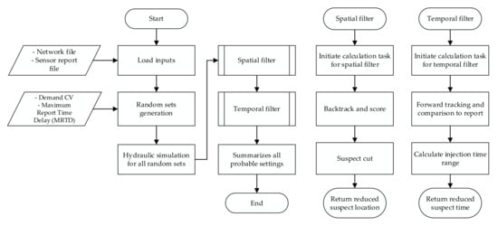
Figure 1.
Contamination-probable setting identifier (CPSITE) calculation flowchart.
2.1. Uncertainties in the CSI Process
A certain degree of uncertainty is always present in the CSI process. In this study, two types of uncertainties for CSI are considered: water flow and sensor report time. Past water flows in pipelines, which are dependent on water consumption at the demand nodes, are required for reverse tracking the contaminant. In general, a demand pattern is assigned to each node for extended-period simulation of a WDN. However, this pattern is different from node to node as each node has various users with different water usage habits. The uncertainty in the sensor report time considered are false-negatives, resulting in a reporting time lag because of calibration errors, network downtime, and data corruption [23].
To include these uncertainties in the proposed CPSITE model, MCS was applied to create random sets of nodal water consumption and sensor report time (representing contaminant arrival time). Because each random set represents a possible situation during the event, it is necessary to evaluate all the random sets to explore possible contamination events. Accordingly, 100 random sets were created and simulated in this study. Note that the number of random sets should be adjusted depending on the network size. The water consumption pattern is generated for each demand node using a normal distribution with a defined coefficient of variation (CV) to quantify the degree of uncertainty in water usage. An example of the generated water consumption patterns is shown in Figure 2. The sensor report time is assumed to have a maximum report time delay (MRTD) of 2 h and follows a normal distribution. For example, if a sensor reported a contamination at 04:00, the contaminant arrival time at the sensor could be between 02:00 and 04:00.
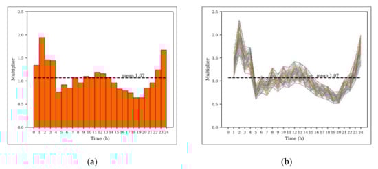
Figure 2.
Nodal water consumption daily pattern: (a) Average pattern and (b) Randomly generated patterns.
2.2. Spatial Filter
As shown in Figure 1, the spatial filter is one of the major focuses of this process and is used to identify every possible suspect injection location (SiL) and suspect injection time (SiT), considering the generated random sets of hydraulic conditions (water flow) and report time. Operations such as backtracking, scoring, and comparison are performed on the generated random sets to minimize the number of SiLs. Backtracking is performed to determine the potential SiLs, and scoring measures the likeliness of each SiL as a true injection point. Subsequently, a comparison process is applied to narrow down the suspects.
Backtracking is applied using a concept similar to that of PBA [6], which begins by initiating a particle at a defined location and time, followed by backtracking the particle in inverse time and path along the pipelines. The particles are split into sub-particles at every junction along the way until all particles finally reach an endpoint (e.g., water source). As the contaminant concentration is excluded, the calculation involves only position tracking across time that requires flow velocity and direction data during the simulation period with the pipe length information.
The overall process of the proposed spatial filter is illustrated in Figure 3 and explained herein. For better explanation of the calculation process, a sample network and sensor report data presented in Figure 4 are used.
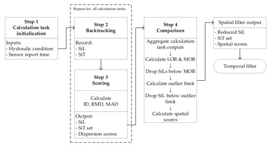
Figure 3.
Calculation flowchart of the spatial filter.
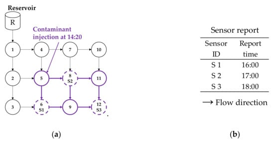
Figure 4.
Sample data for illustration: (a) Sample water distribution network (WDN) and (b) Sensor report time.
The calculation steps for the spatial filter illustrated in Figure 3 are as follows:
Step 1: Initialize calculation task
The calculation task is an individual process with a given input set (i.e., hydraulic condition and sensor report time) that produces the output values (i.e., SiL and SiT). The number of calculation tasks is equal to the number of random sets generated. Steps 2 and 3 describe the process inside each calculation task.
Step 2: Backtracking
Backtracking is conducted on each sensor report location and time using the provided hydraulic condition. Figure 5 shows the backtracking simulation results of the sample network. Backtracking traces the hydraulically connected flow paths and returns the first arrival time (recorded SiT) at every discovered node (recorded SiL). This simulation is conducted on data from all sensors that detect contamination. While analyzing each of the backtracked paths, certain overlapping paths and nodes will be observed (e.g., nodes R, 1, 2, 4, and 5 are identified as SiL from all three sensors, highlighted yellow in the figure and table). Similarly, when combining the results, several SiTs are obtained for each SiL (e.g., Node 5 (SiL) has three SiTs of 14:00, 14:30, and 15:00 obtained from each sensor).
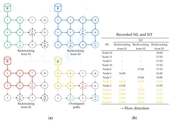
Figure 5.
Backtracking results of the sample network: (a) Backtracking paths and (b) Recorded SiL and SiT.
Step 3: Scoring
A contamination accident is assumed as a single intrusion at a specific location and time to produce the observed outputs. Therefore, a location is more likely to be the true injection point if the calculated SiTs from the sensors are close to each other. For measuring the closeness of the SiTs for each SiL, three measures of statistical dispersion are computed as follows:
- Index of Dispersion (ID): ID is the ratio of variance to the arithmetic mean, as in Equation (1). The value of zero indicates that the obtained SiTs are identical. As the obtained SiTs vary, especially with large outliers, the value will increase.where and are the variance and mean of the SiTs observed at a SiL, respectively.
- Relative mean absolute difference (RMD): RMD compares the mean absolute difference to the arithmetic mean, as expressed in Equation (2). The lowest value of zero indicates an identical data set, and the value increases with dispersion of the SiTs obtained.where is the number of SiTs obtained at a SiL; is the SiT.
- Median absolute deviation (MAD): MAD is a robust measure of dispersion and less affected by outliers. It is defined as the median of the absolute deviations, as expressed in Equation (3). The lower value indicates less dispersion in the obtained SiT values.
Because varies depending on the number of sensors that indicate a node as SiL, the dispersion values with different cannot be treated equally. Hence, a bloat value (BV) is applied to amplify the dispersion value of SiLs detected by fewer sensors. A minimum value is initially assigned to the model. It is a threshold to determine the potential suspects to be considered in the simulation. The SiL with lower than the minimum value is excluded from the dispersion calculation and are automatically assigned a score of zero. Otherwise, the dispersion measures of each SiL are multiplied by BV, which is expressed in Equation (4). Note that by lowing the minimum , the model searches more suspect locations, which may result in longer computation time.
where and are the BV and of the SiL, respectively; is the maximum obtained in the simulation; is the total number of SiLs.
After the three dispersion measures are calculated for all SiLs, each measure is scaled in reverse using a min-max normalization to a value between 0 (more dispersion) and 1 (less dispersion). Then, the three scaled values are summed to represent each SiL by a single likeliness score. Table 1 presents the output from the “Scoring” step containing the information of SiL, SiT, , and the likeliness score.

Table 1.
Scoring process and output results of the sample network.
Step 4: Comparison
The output results from Step 3 (Scoring) vary depending on the random set provided (i.e., hydraulic condition and report time). Steps 1–3 are repeated for a defined number of random sets. In Step 4, we aggregate the output tables from the “Scoring” step obtained for each random set and narrow down the SiLs using Locational Overlap-Rate (LOR) and Maximum Overlap-Rate (MOR) defined in Equations (5) and (6), respectively. The overlap-rate is the number of sensors that detect the same SiL. LOR is the maximum number of sensor detection overlap at a SiL across the random sets, and MOR is the maximum possible detection overlap for all SiLs and random sets. The “Comparison” process of the sample network is shown in Table 2.
where is the LOR for the SiL, is the (number of SiTs) of the SiL in the random set, and is the number of random sets.
When comparing the aggregated results, the SiLs with LOR less than MOR are discarded from the calculation, as seen in Table 2a (Here, MOR is 3, and SiLs with lower than 3 [shown in red box] are discarded). Then, the overall score of the remaining SiLs is calculated by averaging the score from each random set, as shown in Table 2b. The final data cut is executed by a low outlier analysis to remove SiLs with a low score. The low outlier limit is determined as one standard deviation below the mean value, and any SiL with a score below the limit is discarded (e.g., Node R is discarded in Table 2b [shown in red box]). Finally, the spatial score is calculated for the remaining SiL by scaling the scores to values between 0 (least likely) and 1 (most likely). After the spatial filter is applied, nodes 1, 2, 3, 4, and 5 are indicated as the final SiLs, and Node 5 is identified as the most suspicious location (spatial score = 1.0).
2.3. Temporal Filter
After crossing the spatial filter, the final SiLs are narrowed down (e.g., Nodes 1, 2, 3, 4, and 5 for the sample network). The spatial filter outputs the final SiLs with a set of SiTs calculated from the generated random sets, as listed in Table 3. The temporal filter aims to reduce the SiT into a minimized time range for each SiL, as shown in Figure 1. The overall process of the temporal filter is illustrated in Figure 6, followed by the explanations of each step.
Table 3.
Output results from the spatial filter of the sample network.
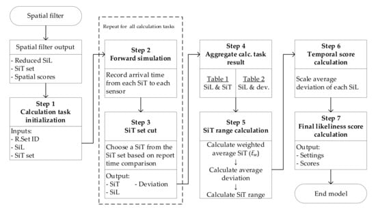
Figure 6.
Calculation flowchart of the temporal filter.
Step 1: Initialize calculation task
A new set of calculation tasks is initiated for the temporal filter. The input to the calculation task is in the form of a random set identifier (R.Set ID), SiL, and SiT set, obtained from the spatial filter. For a single SiL, there will be sets of SiTs equal to the number of random sets, as seen in Table 3. Thus, considering all the SiLs, the number of calculation tasks will be equal to the number of SiLs multiplied by the number of random sets. According to the random set identifier, the related hydraulic condition and sensor report time are loaded into the calculation task for comparison. Steps 2 and 3 describe the process in each calculation task.
Step 2: Forward simulation
The forward simulation is conducted starting from the SiL for each SiT. The contaminant is assumed to be injected into the SiL at SiT, and the contaminant flow paths are traced in the forward time and direction. The first arrival times at the sensor locations are recorded and compared with the sensor report time. Figure 7 illustrates the forward simulation applied to Node 5 of the sample network.
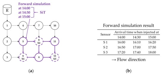
Figure 7.
Forward simulation result of the sample network (Node 5 is a SiL): (a) Forward tracking paths and (b) Arrival times at sensors.
Step 3: SiT set cut
Each forward simulation will create a different set of arrival times for each sensor. Subsequently, the forward-simulated arrival times are compared with the actual report time of each sensor to measure the error (deviation). Figure 8 illustrates the SiT set cut process applied at Node 5, and the descriptions are as follows:
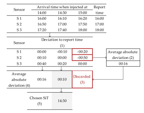
Figure 8.
Suspect injection time (SiT) set cut process of the sample network (Node 5 as a SiL).
- Calculate the deviation between the forward-simulated arrival time and sensor report time for each sensor.
- Calculate the average absolute deviation, and use this value as the false-positive limit.
- Discard the SiTs that induce arrival times exceeding the defined false-positive limit.
- Calculate the average absolute deviation for each SiT.
- Select the SiT that results in the lowest deviation for all sensors.
The output from the calculation task (Steps 2–3) is the chosen SiT for the SiL and the lowest average absolute deviation for each random set (for example, from Figure 8, SiL = Node 5, chosen SiT = 14:30, and Dev. = 00:10). Steps 2–3 are repeated for the defined number of calculation task sets.
Step 4: Calculation task results aggregation
After finishing all the calculation tasks, the results of SiT and deviation values are compiled into two tables, as shown in Table 4. For the SiLs and random sets, Table 4a lists the finally chosen SiT, and Table 4b lists the deviation value.
Step 5: SiT range calculation
To estimate the SiT range of each SiL, an analysis of the injection time spread is conducted. As each SiT has a certain deviation value (as seen in Table 4), they have different relative importance. Hence, the weighted average SiT of each SiL is calculated using Equation (7) as follows:
where is the weighted average SiT, is the SiT; is the deviation value.
The average deviation values are then calculated and applied to the weighted average SiT () to create the minimum and maximum SiT range. Figure 9 illustrates the SiT range of Node 5 (SiL) in the sample network. The SiT values (blue line) are sorted in ascending order along with the corresponding deviation values (the two green lines represent the upper (=SiT + Dev.) and lower limits (=SiT − Dev.)). After applying Equation (7), the weighted average SiT () is found to be 14:27 (dash-dot red line), and the average deviation was calculated to be 26 min. Thus, the final SiT ranges from 14:01 to 14:53, as indicated in the shaded interval in Figure 9.
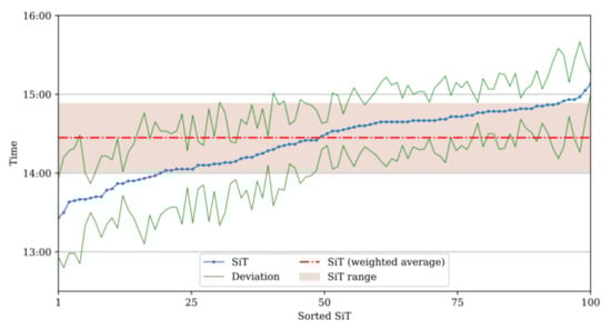
Figure 9.
SiT range calculation for Node 5 (SiL) in the sample network.
Step 6: Temporal score calculation
After estimating the SiT range for each SiL, a temporal score is calculated by scaling the average deviation into values between 0 (least likely) and 1 (most likely), as shown in Table 5.
Table 5.
Temporal score calculation of the sample network.
Step 7: Final score calculation
The final score of each SiL is calculated by averaging both the spatial and temporal scores. The final score serves as a likeliness index of a set (i.e., SiL and SiT). The final output of the CPSITE simulation is the list of the SiL, SiT range, and the scores, as shown in the highlighted sections of Table 6. Node 5 is identified as the most suspicious location (final score = 1.0) with the potential injection time range of 14:01–14:53.
Table 6.
Final output of CPSITE simulation for the sample network.
3. Application
The calculations in this study were performed using the Python 3 programming language [24], supported with Water Network Tool for Resilience (WNTR) 0.2.2.1 Python package to utilize the EPANET hydraulic simulation model [25]. The program was run using an Intel Core i7-8700 CPU @ 3.2 GHz (12 CPUs) and 16 GB RAM on a Windows 10 environment. Multiprocessing was enabled using the Python multiprocessing package to use multiple CPUs to pool the calculation tasks and reduce the computation time.
3.1. Contamination Scenarios
To demonstrate CPSITE, EPANET Example Network 3 (NET3) was used as an application WDN, as shown in Figure 10. NET3 consists of 91 junctions, 2 reservoirs, 3 tanks, 115 pipes, and 2 pumps. Sensor placement in the network was based on the example of the threat ensemble vulnerability assessment and sensor placement optimization tool (TEVA-SPOT) [26]. The demand pattern representing the temporal water consumption of individual nodes was adapted from the original network. CPSITE is dependent on the sensor response. Therefore, three single-injection scenarios with different injection locations and times to produce different sensor responses were created to evaluate the model capability. The random set generation parameters were set to default values; the CV was set to 0.2 for water consumption uncertainty with an MRTD of 2 h. Figure 10 depicts the network layout and the five sensor locations.
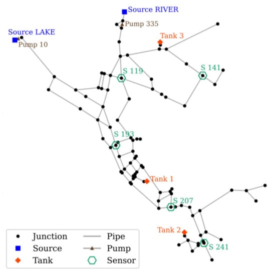
Figure 10.
Application network layout and sensor location.
3.1.1. Scenario 1
The data used for scenario 1 are provided in Table 7. Figure 11 presents the model simulation results. The true contaminant injection occurred via Node 101 at 04:00, and contamination was detected by all sensors. The first and last reading sensors are S193 (at 05:45) and S141 (at 14:45), respectively. The report time delay was calculated by comparing the sensor report time with the true arrival time of the contamination. The shortest and longest delays were simulated to be 15 min and 1 h 15 min, respectively, with an average of 48 min.
Table 7.
True injection and sensor information (scenario 1).
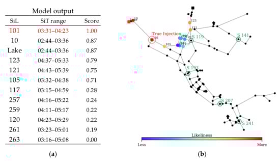
Figure 11.
CPSITE simulation results of scenario 1: (a) Model output and (b) SiL layout.
The model indicated 12 SiLs during the simulation. The SiT range and the likeliness score of each SiL are provided in Figure 11. The most likely injection location is identified as Node 101, which coincides with the true injection point. Regarding the injection time estimation, the model yielded an injection time range of 03:31–04:23 for Node 101, which is close to the true injection time of 04:00. The model runtime for this scenario with 100 random sets was 14 min.
3.1.2. Scenario 2
The information applied for scenario 2 is provided in Table 8, and the simulation results are presented in Figure 12. The true injection point (Node 259) is located in the middle upstream area between the two sources. The contaminant was injected at 12:00, and four sensors (except S141) detected the contamination, with the first and last readings being S119 (at 13:49) and S241 (at 21:55), respectively. The shortest and longest delays were simulated as 39 min and 2 h, respectively, with an average of 1 h 4 min.
Table 8.
True injection and sensor information (scenario 2).
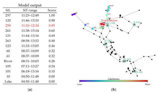
Figure 12.
CPSITE simulation results of scenario 2: (a) Model output and (b) SiL layout.
The simulation of the given contamination scenario identified 14 SiLs, as shown in Figure 12. Among these, Node 257 is identified as the most probable injection point, which is very close to the true injection location (Node 259). The topmost three SiLs (Nodes 257, 120, and 259) are in close proximity, as shown in Figure 12. Although the model fails to pinpoint the true injection location, it localizes a small high likelihood area containing the true injection point. Regarding the injection time estimation, the model provided an injection time range of 11:10–12:34 for Node 259, which contains the true injection time of 12:00. The model runtime for this scenario with 100 random sets was 16 min.
3.1.3. Scenario 3
The data generated for scenario 3 are presented in Table 9, and the simulation results are illustrated in Figure 13. The true injection point is located in the middle of the network at Node 113. In this event, only three sensors detect contamination (S193, S207, and S241). Given an injection time of 06:00, the first and last reports are from sensors S193 (at 07:30) and S241 (at 11:00), respectively. The shortest report delay was 1 h, and the longest report delay was 1 h 20 min, with an average of 1 h 13 min.
Table 9.
True injection and sensor information (scenario 3).
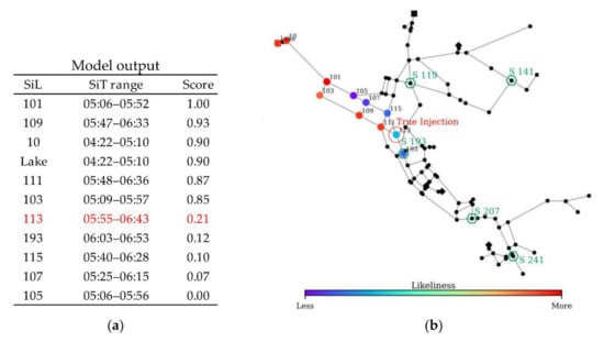
Figure 13.
CPSITE simulation results of scenario 3: (a) Model output and (b) SiL layout.
The model simulation yielded 11 SiLs, with Node 101 identified as the most suspicious location, which is far upstream from the true injection node (Node 113). The model failed to pinpoint the true injection node and localize the potential area in this scenario. As observed in Figure 13, though the true injection node is identified as an SiL, the likeliness score is minimal (0.21) because of two factors. First, the available sensor report information was not sufficient because only three sensor reports were utilized. Second, the sensor reports were all delayed for more than 1 h, thereby making the upstream node as the most suspicious location. This scenario reveals that sensor information (e.g., number of sensor reports, sensor layout, and sensor accuracy) significantly affects model performance. The simulation time for this scenario with 100 random sets was 5 min, which is considerably lower than that for the previous scenarios. This indicates that the model simulation time depends on the number of reporting sensors and identified SiLs.
3.2. Effects of Degree of Uncertainty
The variations in model performance depend on the uncertainties contained in the water flows and sensor report time. CPSITE employs two parameters for randomizing water flow (or water consumption) and sensor report time. The CV of water demand quantifies the degree of uncertainties in water flow and was varied from 0.0 to 0.3. The MRTD was assumed to be between 2 and 3 h. With a real injection time of 04:00 at Node 101 of scenario 1, the sensitivity analyses were performed using CPSITE. The results are summarized in Table 10.
Table 10.
Sensitivity analysis of water flow and sensor report uncertainty.
The MRTD has a significant impact on the simulation results, while the demand CV produces marginal changes. Regardless of the demand CV, if MRTD is 2 h, the model accurately identified the true injection point, and the weighted average SiT () is in closest proximity to the true injection time, with temporal deviation less than 30 min. However, if MRTD increases to 3 h, the model fails to specify the true injection point and SiT range becomes wider (the temporal deviation is more than 1 h). This behavior shows that the sensor information (represented by MRTD) has a considerable effect on the model performance than the water flow information (represented by demand CV). The demand CV controls the variation of individual nodal demands, thereby changing the flow (i.e., velocity) in pipes, affecting the contaminant particle travel time and possibly the direction. However, increasing the value only provides more SiLs as more possible travel paths can be determined. It renders no significant changes in the time-related results (i.e., SiT, Δt to true injection time, and average deviation), particularly for the top scorer.
The runtime of CPSITE is related to several factors, such as the number of reporting sensors, number of SiLs determined, and number of random sets for uncertainty analysis. Given fixed sensor layouts and random sets, the runtime is undoubtedly related to the number of SiLs, as presented in Table 10. The model runtime is important in a CSI problem to adopt prompt action for isolating the contaminated area and setting up the washing-out strategies to minimize the damage.
3.3. Effects of Sensor Availability
Because of the malfunctioning issue, certain sensors may be unavailable during the contamination event. Based on scenario 2, three sub-scenarios of malfunctioning sensors or data corruption were created without changing the report time. Among the five sensors installed, four sensors were available for scenario 2, and only three sensors were available for sub-scenarios 2(a)–2(c), as indicated in Figure 14. Furthermore, this illustrates how the interaction of different sensor combinations can affect the simulation results. The default uncertainties were applied for the simulations (i.e., demand CV and MRTD were set to 0.2 and 2 h, respectively). Figure 14 illustrates the CPSITE simulation results of the four scenarios (scenario 2 and three sub-scenarios). The summary results are listed in Table 11.
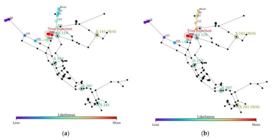
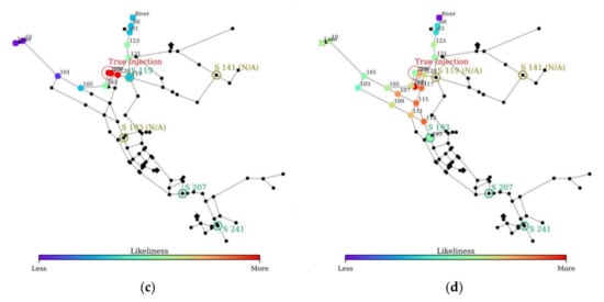
Figure 14.
CPSITE simulation results: (a) Scenario 2, (b) Scenario 2a, (c) Scenario 2b, and (d) Scenario 2c.
Table 11.
Summary of scenario 2 and the sub-scenario results.
Overall, scenario 2 and the two sub-scenarios (i.e., scenarios 2a and 2b) yield similar performance for identifying the true injection point and time range. They identified approximately the same SiLs; however, the likeliness increases for the SiLs located near the source (River) in scenario 2a. Meanwhile, scenario 2c exhibits the worst model performance compared to the other three scenarios. In this scenario, two upstream sensors are unavailable, resulting in more SiLs identified, thereby decreasing the rank and score significantly. Nevertheless, even with the reduced sensor availability, the model can result in a SiT close to the true injection time (at 12:00) for all sub-scenarios.
3.4. Contaminant Spread over Time
The identified contamination setting (i.e., SiL and SiT) can be used to estimate the contaminated area in the network at certain times. The area contaminated by the three high-ranked SiLs and the corresponding SiT ranges in scenario 2 are estimated and compared in Figure 15. The actual contamination path by the true injection location and time (Node 259 at 12:00) are also identified in the figure for comparison. The potentially contaminated area was estimated using a forward simulation for all the random sets of water flow to determine the maximum possible range. Figure 15 depicts the extent of contamination for three different settings over time.
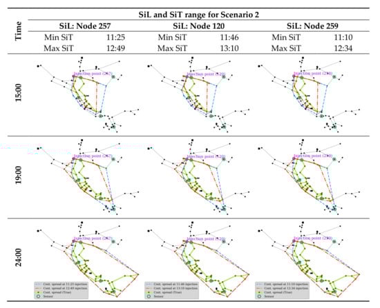
Figure 15.
Spatiotemporal contamination extent by three contamination settings found in Scenario 2.
All the estimated contamination areas by different settings exhibit a close match with the actual boundary at every time point. This reveals that the model can predict the potential boundary of the contaminated area after localizing the suspect injection point and time. Consequently, the damaged area will be isolated, and proper treatment can be applied. As observed in Figure 15, the minimum-SiT area (blue line) naturally provides more coverage as it is the earliest injection. However, the maximum-SiT area (red line) exists outside at certain time points owing to different hydraulic conditions over time. The actual contamination path is well-contained within the minimum and maximum boundaries predicted by the CPSITE simulation.
4. Conclusions
The CPSITE model was developed to identify the suspect location and time of a contaminant intrusion, considering uncertainties in water flow and sensor report time. The model regards the network and sensor report data as inputs, applies MCS to create random sets of water consumption and sensor reports, and then applies the novel spatial and temporal filters to identify the possible contamination setting. Both filters are based on result comparison. The spatial filter employs backtracking to acquire all possible SiLs and SiTs, thereby focusing on reducing the number of SiL. Afterward, the temporal filter utilizes forward simulation to identify the potential range of the SiT. The final outcome from the model is a list of SiL with SiT range and the likeliness score.
The model performance is demonstrated by applying three single-injection scenarios to the well-known NET3, with different injection locations and times. In all scenarios, the true injection locations and times were well-identified within the set of SiLs and SiT ranges. However, the model performance substantially depended on the accuracy of the available sensor information. The CPSITE simulation time was primarily dependent on the number of SiLs identified. Sensitivity analyses were conducted to quantify the effects of uncertainties in water flow and sensor report time. The results reveal that, compared to the water flow variation (represented by demand CV), the sensor accuracy (represented by MRTD) has a considerable effect on the model performance. In addition, the effect of sensor availability was investigated. The sensor location and availability were proved to contribute significantly to the model. However, CPSITE could identify the contamination setting with a reduced number of available sensors. The model performance would be affected by the network characteristics such as size and type. That is, larger networks would require longer computation time to obtain the suspects, and more densely looped networks would result in wider range of suspects in space and time. After identifying the intrusion location and time, the model could predict the contaminated area in the network over time, and it matched appropriately with the actual contamination boundary.
The proposed model can efficiently discover the possible intrusion location and time of a contaminant, considering the uncertainties in the given data. Furthermore, the results can predict the extent of contamination to estimate the damage and plan a strategy for valve closure for efficiently draining contaminated water. Future studies should ideally aim to optimally locate the sensors, because sensor information significantly affects model performance. The proposed model can be further extended by simulating the contaminant concentration and modifying the filter processes to consider the possibilities of multiple contamination sources.
Author Contributions
Conceptualization, M.S.M. and D.K.; methodology, M.S.M. and D.K.; coding and simulation, M.S.M.; writing—original draft preparation, M.S.M.; writing—review and editing, D.K.; supervision, D.K.; funding acquisition, D.K. All authors have read and agreed to the published version of the manuscript.
Funding
This work was supported by (1) the National Research Foundation of Korea (NRF) grant funded by the Korean government (MSIT—Ministry of Science and ICT) (No. NRF-2020R1A2C2009517); and (2) the EDISON (Education-research Integration through Simulation On the Net) Program through the National Research Foundation of Korea (NRF) funded by the Ministry of Science, ICT, and Future Planning (2017M3C 1A6075016).
Conflicts of Interest
The authors declare no conflict of interest.
References
- Kirmeyer, G.J.; Martel, K. Pathogen Intrusion into the Distribution System; American Water Works Association: Denver, CO, USA, 2001. [Google Scholar]
- Rasekh, A.; Hassanzadeh, A.; Mulchandani, S.; Modi, S.; Banks, M.K. Smart water networks and cyber security. J. Water Res. Plan. Man. 2016, 142, 01816004. [Google Scholar] [CrossRef]
- Hu, C.; Zhao, J.; Yan, X.; Zeng, D.; Guo, S. A MapReduce based Parallel Niche Genetic Algorithm for contaminant source identification in water distribution network. Ad. Hoc. Netw. 2015, 35, 116–126. [Google Scholar] [CrossRef]
- Adedoja, O.S.; Hamam, Y.; Khalaf, B.; Sadiku, R. Towards development of an optimization model to identify contamination source in a water distribution network. Water 2018, 10, 579. [Google Scholar] [CrossRef]
- Zierolf, M.L.; Polycarpou, M.M.; Uber, J.G. Development and autocalibration of an input-output model of chlorine transport in drinking water distribution systems. IEEE Trans. Cont. Syst. Technol. 1998, 6, 543–553. [Google Scholar] [CrossRef]
- Shang, F.; Uber, J.G.; Polycarpou, M.M. Particle backtracking algorithm for water distribution system analysis. J. Environ. Eng. 2002, 128, 441–450. [Google Scholar] [CrossRef]
- Laird, C.D.; Biegler, L.T.; van Bloemen Waanders, B.G.; Bartlett, R.A. Contamination source determination for water networks. J. Water Res. Plan. Man. 2005, 131, 125–134. [Google Scholar] [CrossRef]
- Laird, C.D.; Biegler, L.T.; van Bloemen Waanders, B.G. Mixed-integer approach for obtaining unique solutions in source inversion of water networks. J. Water Res. Plan. Man. 2006, 132, 242–251. [Google Scholar] [CrossRef]
- De Sanctis, A.E.; Shang, F.; Uber, J.G. Real-time identification of possible contamination sources using network backtracking methods. J. Water Res. Plan. Man. 2010, 136, 444–453. [Google Scholar] [CrossRef]
- Preis, A.; Ostfeld, A. A contamination source identification model for water distribution system security. Eng. Optim. 2007, 39, 941–947. [Google Scholar] [CrossRef]
- Rossman, L.A. EPANET 2: Users Manual; National Risk Management Research Laboratory: Cincinnati, OH, USA, 2000. [Google Scholar]
- Liu, L.; Ranjithan, S.R.; Mahinthakumar, G. Contamination source identification in water distribution systems using an adaptive dynamic optimization procedure. J. Water Res. Plan. Man. 2011, 137, 183–192. [Google Scholar] [CrossRef]
- Yan, X.; Zhao, J.; Hu, C.; Wu, Q. Contaminant source identification in water distribution network based on hybrid encoding. J. Comput. Meth. Sci. Eng. 2016, 16, 379–390. [Google Scholar] [CrossRef]
- Yan, X.; Gong, W.; Wu, Q. Contaminant source identification of water distribution networks using cultural algorithm. Concurr. Comput. 2017, 29, e4230. [Google Scholar] [CrossRef]
- De Sanctis, A.E.; Boccelli, D.L.; Shang, F.; Uber, J.G. Probabilistic approach to characterize contamination sources with imperfect sensors. In Proceedings of the World Environmental and Water Resources Congress 2008, Ahupua’A, HI, USA, 12–16 May 2008; pp. 1–10. [Google Scholar]
- Yang, X.; Boccelli, D.L. Bayesian approach for real-time probabilistic contamination source identification. J. Water Res. Plan. Man. 2014, 140, 04014019. [Google Scholar] [CrossRef]
- Perelman, L.; Ostfeld, A. Bayesian networks for source intrusion detection. J. Water Res. Plan. Man. 2013, 139, 426–432. [Google Scholar] [CrossRef]
- Vankayala, P.; Sankarasubramanian, A.; Ranjithan, S.R.; Mahinthakumar, G. Contaminant source identification in water distribution networks under conditions of demand uncertainty. Environ. Forensic. 2009, 10, 253–263. [Google Scholar] [CrossRef]
- Preis, A.; Ostfeld, A. Hydraulic uncertainty inclusion in water distribution systems contamination source identification. Urban. Water J. 2011, 8, 267–277. [Google Scholar] [CrossRef]
- Preis, A.; Ostfeld, A. Genetic algorithm for contaminant source characterization using imperfect sensors. Civ. Eng. Environ. Syst. 2008, 25, 29–39. [Google Scholar] [CrossRef]
- Tao, T.; Huang, H.D.; Xin, K.L.; Liu, S.M. Identification of contamination source in water distribution network based on consumer complaints. J. Cent. South. Univ. 2012, 19, 1600–1609. [Google Scholar] [CrossRef]
- Hill, J.; van Bloemen Waanders, B.; Laird, C. Source inversion with uncertain sensor measurements. In Proceedings of the ASCE Water Distribution Systems Analysis, Cincinnati, OH, USA, 27–30 August 2006. [Google Scholar]
- Bristow, E.C.; Brumbelow, K. Delay between sensing and response in water contamination events. J. Infrastruct. Syst. 2006, 12, 87–95. [Google Scholar] [CrossRef]
- van Rossum, G.; Drake, F.L., Jr. Python Reference Manual; Centrum voor Wiskunde en Informatica: Amsterdam, The Netherlands, 1995. [Google Scholar]
- Klise, K.A.; Hart, D.; Moriarty, D.; Bynum, M.L.; Murray, R.; Burkhardt, J.; Haxton, T. Water Network Tool for Resilience (WNTR) User Manual; Sandia National Laboratories: Albuquerque, NM, USA, 2017. [Google Scholar]
- Berry, J.; Booman, E.; Riesen, L.A.; Hart, W.E.; Phillips, C.A.; Watson, J.P.; Murray, R. User’s Manual: TEVA-SPOT Toolkit 2.4; EPA 600/R-08/041B; National Homeland Security Research Center, U.S. EPA: Washington, DC, USA, 2010.
Publisher’s Note: MDPI stays neutral with regard to jurisdictional claims in published maps and institutional affiliations. |
© 2020 by the authors. Licensee MDPI, Basel, Switzerland. This article is an open access article distributed under the terms and conditions of the Creative Commons Attribution (CC BY) license (http://creativecommons.org/licenses/by/4.0/).