Article

Optimization of the Multi-Start Strategy of a Direct-Search Algorithm for the Calibration of Rainfall–Runoff Models for Water-Resource Assessment

by
Liliana García-Romero
1,*,
Javier Paredes-Arquiola
1,
Abel Solera
1,
Edgar Belda
1,
Joaquín Andreu
1 and
Sonia T. Sánchez-Quispe
2,*
1
Research Institute of Water Environmental Engineering (IIAMA), Universitat Politècnica de València, 46022 Valencia, Spain
2
Faculty of Civil Engineering, Universidad Michoacana de San Nicolás de Hidalgo, Morelia 58030, Mexico
*
Authors to whom correspondence should be addressed.
Water 2019, 11(9), 1876; https://doi.org/10.3390/w11091876
Submission received: 2 August 2019 / Revised: 22 August 2019 / Accepted: 5 September 2019 / Published: 9 September 2019
(This article belongs to the Section Water Resources Management, Policy and Governance)

Abstract

:
Calibration of conceptual rainfall–runoff models (CRRM) for water-resource assessment (WRA) is a complicated task that contributes to the reliability of results obtained from catchments. In recent decades, the application of automatic calibration techniques has been frequently used because of the increasing complexity of models and the considerable time savings gained at this phase. In this work, the traditional Rosenbrock (RNB) algorithm is combined with a random sampling method and the Latin hypercube (LH) to optimize a multi-start strategy and test the efficiency in the calibration of CRRMs. Three models (the French rural-engineering-with-four-daily-parameters (GR4J) model, the Swedish Hydrological Office Water-balance Department (HBV) model and the Sacramento Soil Moisture Accounting (SAC-SMA) model) are selected for WRA at nine headwaters in Spain in zones prone to long and severe droughts. To assess the results, the University of Arizona’s shuffled complex evolution (SCE-UA) algorithm was selected as a benchmark, because, until now, it has been one of the most robust techniques used to solve calibration problems with rainfall–runoff models. This comparison shows that the traditional algorithm can find optimal solutions at least as good as the SCE-UA algorithm. In fact, with the calibration of the SAC-SMA model, the results are significantly different: The RNB algorithm found better solutions than the SCE-UA for all basins. Finally, the combination created between the LH and RNB methods is detailed thoroughly, and a sensitivity analysis of its parameters is used to define the set of optimal values for its efficient performance.

1. Introduction

Hydrological modelling is essential for water-resource assessment (WRA) [1]. Hydrologists have come to rely on hydrological models to foresee events that would otherwise be difficult to predict [2]. Estimating flows that run in a basin through a drainage system is one of the greatest tools available to address hydrological problems [3].
Currently, there are many hydrological models that can be used for WRA [4]. Conceptual rainfall–runoff models (CRRM) are often used, because they offer simplified catchment-scale representations of the transformation of precipitation into river discharge [5]. Their efficient calibration is a difficult issue, even for experienced hydrologists [6]. The models are characterised by parameters that cannot be directly measured in the field. However, they can be inferred by the so-called calibration process [7]. During this phase/process, parameters are estimated indirectly by minimizing the discrepancy between direct simulated and observed model outputs [8]. Moreover, the success of the application of CRRM depends on the degree of calibration achieved and the choice of suitable calibration strategies [9,10].
To estimate the parameter values, manual calibration is one option. However, it is a time-consuming and very laborious phase. The process is sometimes still used [11,12,13]. However, when complex models are used, it is practically impossible to perform a manual calibration to find the best possible parameter set. An alternative is to use automatic calibration algorithms [14,15], which make model calibration easier and faster. This technique automatically enhances the quality of manual calibration, providing a significant improvement [14]. Currently, there are many automatic calibration algorithms available. Some are modern or recent algorithms (developed in the last decade), and others are traditional or historical algorithms (developed from 1965 until the last decade) [16,17]. However, they do not offer the same performance levels [2].
During the last decade, several papers comparing optimization algorithms applied to CRRM calibration were published to prove or disprove the efficiency of a particular modern or historical method [2,16,17,18,19]. In studies by Sörensen [20] and Piotrowski et al. [17], they contended that they did not consider such an uncontrolled increase in the number of supposedly new algorithms to be a positive research trend. In studies by [16,20,21,22,23,24,25,26,27,28,29,30], it was found that, generally, modern algorithms, can become completely unreliable on specific problems, even though they perform reasonably on others. Furthermore, traditional algorithms, such as the Rosenbrock (RNB) or Nelder–Mead (NM), have proven surprisingly efficient compared to modern algorithms.
The RNB algorithm [31] is a historical technique analysed in many comparisons of optimization algorithms since its development until the present [19]. For example, with an internal modification made for hydrological models using synthetic error-free data, the method was found to be robust by [32], who conducted a study comparing nine different methods for fitting hydrological models. In the study of [33] used the technique for illustrating the application of linear rainfall–runoff models in 14 catchments. Moreover, Liang et al. [34] demonstrated the application of two linear flow-routing methods on three rivers in China.
Also Goswami and O’Connor [18] tried the RNB algorithm and five additional different optimization techniques in the calibration of two catchments. They found that the direct-search methods (e.g., RNB) were efficient in terms of fewer numbers of objective functions (OF) evaluations necessary to find the best solution, making them very fast algorithms. However, in some cases, they were trapped in local-optimal solutions. In that study, the RNB algorithm was started sequentially from each point of a large sample of points in the parameter space, each aiming to reach the optimum [35,36,37]. By launching it from each point, the computational time consumed was excessive, and the algorithm was unable to come out of the local optimum in some cases. The direct-search methods use only OF values. Thus, it is not necessary to perform derivatives [31,38,39,40]. Therefore, it can be applied to many cases. However, one of the main problems in these techniques is the presence of multiple local solutions that can cause the algorithm to be unable to find the global solution of the problem [41]. In this sense, the application of local-search methods has been tried by leveraging the re-initialization of the algorithm at some randomly selected points [42,43], allowing a roughly homogeneous exploration of the sample space [16].
Thirty optimization heuristics algorithms were tested by Piotrowski [22] to evaluate artificially constructed benchmark functions. Among them were two traditional local-search algorithms (i.e., RNB and NM) [39], which were compared with results obtained from the other 28 methods. Both algorithms were applied with a re-initialization, depending on the number of OF calls. Interestingly, both algorithms performed as well as the modern techniques. In fact, this study suggests that testing traditional algorithms as RNB in other fields may be interesting.
Moreover, Piotrowski et al. [17] evaluated the performance of 33 optimization algorithms (e.g., RNB and NM). They analysed the performance versus the speed of each algorithm in the solution of 22 numerical real-world problems from different fields of science with the maximum number of OF calls varying between 5000 and 500,000. They found that the historical algorithms outperformed recent algorithms, even when they were based on the first ones. Moreover, the RNB algorithm was more specialized, fast and one of the best for solving hydraulic engineering problems.
Recently, Piotrowski et al. [16] compared 26 algorithms created from 1970 to the present, including a number of modern evolutionary or swarm-intelligence methods and traditional techniques such as the RNB algorithm. These methods were used on the calibration of two different CRRMs in four catchments located in roughly similar climatic conditions on two continents. It was found that, generally, nearly all algorithms performed similarly on each calibration problem, and no method could be called superior to others in terms of final performance. It was also shown that the historical direct-search methods performed equally well in finding the best solutions as modern optimizers. These methods were implemented with a re-initialization at two points selected randomly but without any previous analysis. Thus, with the RNB method, after 100 D (where D is the dimensionality of the problem) function calls are verified; if, during the last 100 D function calls, the solution is improved by more than 1 × 10⁻⁴, then the optimal solution is found. Otherwise, the location of the RNB point is randomly re-initialized again from a random starting point. The value of the step length is re-set to 0.1 [31], and the coordinates are re-set to the initial system. This conceptualization allows the use of randomization resources to better explore the sample space and find global solutions without previous analysis of the initial points.
In summary, in the studies discussed, we found that modern and historical algorithms provided similar results in the solution of the same problem. Even RNB proved to be more efficient than some modern metaheuristics in finding optimal solutions with higher speed. The study [2] established that the best methods were those that converged to a better-quality minimum as rapidly as possible. However, the problem with the direct-search methods was that it could be trapped in local-optimal solutions if the random re-initialization missed. These methods have been known for many years [44], but currently the popularity of so-called metaheuristics is soaring in hydrology [21,45]. However, these algorithms have been analysed over the last decade, showing that, at least, some of them mimic the traditional methods, lack any true novelty, or are developed without scientific rigor [20,22,46,47].
Because of complications regarding local-search algorithms and because of the introduction of the University of Arizona’s shuffled complex evolution (SCE-UA) method by Duan et al. [9], used to locate the global optimum of a CRRM, many researchers in hydrology have employed this for parameter optimization [24,48,49,50,51,52]. Some studies have shown that it is a robust and efficient algorithm [41], whereas its efficiency has been evaluated by comparing it with many others [2,18,53]. In fact, this algorithm has become the method of choice to solve runoff model calibration problems [7]. Recently, this technique demonstrated that, in spite of being an algorithm developed in the 1990s, its results were efficient and reliable, playing a key role in analysing the relationship between calibration time and final performance of several algorithms that calibrate CRRMs [19,54].
Based on these studies, we have summarized several key points. There is no algorithm that solves all problems correctly and efficiently [21]. Therefore, it is important to explore the behaviour of some algorithms in the solution of any problem. Historical algorithms can behave the same or better than modern algorithms in solving specific problems and some authors have argued that it would be interesting to test these methods in different cases [22]. Finally, we identified that the RNB algorithm proposed during the 1960s used with a simple restart method was still competitive and, in some cases, better than some recent algorithms [17].
Moreover, Chlumecký et al. [6] suggested that a method allowing the exploration of the sample space or a selection of random values as starting points could improve results. Therefore, we decided to improve the use of RNB with the initial application of a random sampling method (Latin hypercube (LH)). This should enable the controlled exploration of the total solution space addressed in the problem and select only the best points after a previous OF analysis. The RNB algorithm will be re-initialized, but only as many times as necessary from the best sorting points, thereby saving considerable computational time. In previous studies in which RNB was used, algorithm re-initialization at uncontrolled random points was conducted. This re-initialization depended on specific OF call numbers or a pre-defined number of re-sets (one or two), but not from a probability analysis of the solution space.
Therefore, the aim of this paper is to test the ability of a direct-search algorithm, RNB, combined with the LH method designing a controlled multi-start strategy for the calibration of CRRMs with different complexities in the WRA. We explain the mathematical relationship between the two methods, because this aspect has not been addressed in the literature. Moreover, a detailed sensitivity analysis of parameters of coupled techniques is made, setting optimal parameter values to solve problems of CRRM calibration. To assess the performance of this technique, the SCE-UA algorithm is used as a benchmark, because it has proven to be a robust technique in the calibration of CRRMs.
Finally, the focus in the application of this algorithm is oriented to the applicability of WRA for the management of complex systems and not for the analysis of flood events, which are regularly the cases that have been more frequently analysed [55,56].

2. Materials and Methods

2.1. Case Study and Data

The present study is based on data collected from nine headwaters of the Duero and Júcar River Basin Districts in Spain (Figure 1). These catchments are located in areas that commonly present severe droughts because of climatological conditions and geographical locations [57,58,59]. The catchment areas in the Júcar system are zones characterized by a semi-arid climate [60]. The Duero system contains zones characterized by a Mediterranean climate with temperate and rainy winters, but very dry and warm summers. Thus, the evaluation of water resources in these exploitation systems is an essential action.
Four basins in the Duero system have the presence of snow (Table 1) that accumulates from late autumn to spring, reaching a maximum depth and duration during the winter months. The snowmelt begins in the spring and summer when the precipitation is otherwise scarce. Thus, it is important to consider the modelling process [61].
The climatological, hydrological and morphological characteristics are different in each basin (Table 1). Every case-study catchment has a gauging station and a series of observed flows of at least 10 years of data without the need to complete or extend the data series. In Table 1 we assigned a number to each basin. From this point, we refer to them by this number and not by their name.
To add the least amount of noise to the modelling process, only headwater basins were selected, because they are the zones where the runoff data have the minimal anthropogenic alteration, and the capacity of the algorithms can be tested homogeneously without noise resulting from the data.
Daily series of precipitation (P) were obtained from the Spain02 database [62] at a grid resolution of 0.2° (approx. 20 km). The State Meteorological Agency and the Meteorology Group of Santander in Spain prepared this dataset jointly. Potential evapotranspiration (PE) was calculated using the Hargreaves and Samani method [63] and the temperature series obtained from the aforementioned database. The observed daily flows were obtained from the Information System of the Discharges Yearbook of the Ministry of Agriculture and Fisheries, Food and Environment of the Government of Spain [64].

2.2. Conceptual Rainfall–Runoff Models

In this section, we describe three lumped conceptual models (i.e., the French rural-engineering-with-four-daily-parameters (GR4J) model, the Swedish Hydrological Office Water-Balance Department (HBV) model and the Sacramento Soil Moisture Accounting (SAC-SMA) model) used to test the design multi-start strategy of a direct-search algorithm during the calibration stage. The models involve a configuration of interconnected stores with mathematical transfer functions used to direct the movement of water in a basin. Each has a different structural complexity, a different number of parameters (4, 8 and 16) and a specific mathematical formulation. Their selection was based on their successful application in WRA studies [50,65,66,67,68]. The parameter ranges for each model are based on experience and the literature review [69,70,71,72]. We applied these models using the open and freely available software ‘EVALHID’ Water Resources Assessment, version 1.3, [73] developed by the Universitat Politècnica de València in Valencia, Spain.

2.2.1. French Rural-Engineering-with-Four-Daily-Parameters (GR4J) Model

The GR4J model is a lumped, conceptual, daily model developed by [72], belonging to the family of soil-moisture accounting models. It performs well even for data within short time intervals ref. [74] or practically ungauged catchments [75]. The GR4J model is represented by two tanks: production and routing. It is controlled by four parameters (description in Appendix A Table A1). For a detailed mathematical explanation see [72].

2.2.2. Swedish Hydrological Office Water-Balance Department (HBV) Model (with the Snow Component)

The HBV model [70] is a lumped, conceptual and daily model that simulates discharge in the catchment using rainfall, temperature (if applicable) and estimates of potential evaporation. It has been used in more than 30 countries under different climatic conditions. The model simplicity of the input data, and the robust model structure have demonstrated reliable performance in solving water-resource problems [76].
The model comprises three primary routines: first is snow accumulation and melt, which is computed by a simple degree-day method, where a threshold temperature (usually close to 0°) is defined at the location above where snow melt occurs [77]. Second is a soil moisture accounting routine that computes an index of the wetness and soil moisture storage in a catchment. Third is a response routine that transforms excess water from the soil moisture routine to discharge to each sub-basin. There are two reservoirs connected in series by a constant percolation rate. Generally, the input variables are daily P, estimated PE and mean-air temperature when the snow module is applied. The model is controlled by eight parameters for rain and two for snow (see parameter description in Appendix A Table A1). The model equations of HBV (including snow routine) can be found in other works [70,77,78].
The snow routine described here is used as a model for the four basins with this component. It uses, simultaneously, the reduction in the dimensionality of the problem.

2.2.3. Sacramento Soil Moisture Accounting (SAC-SMA) Model

The SAC-SMA model [71] is a conceptual water-balance physical model based on the principles of water movement in a catchment. It is one of the most widely used rainfall–runoff model [79]. It works by using a system of water reservoirs (zones). The basic design incorporates two soil-layer structures. Each comprises tension and free-water reservoirs that interact to generate soil moisture, and there are five runoff components. The total streamflow is the sum of all partial runoffs. The model was configured with 16 calibration parameters described in Appendix A Table A1. A detailed mathematical analysis of the model can be found in [71].

2.3. Optimization Methods

In this section, the optimization methods used to calibrate CRRMs are described. First, we explain in detail the linking of the RNB algorithm to the random sampling method, LH, to create a multi-start strategy of a direct-search algorithm. Next, we describe the SCE-UA algorithm that was selected as a benchmark method.

2.3.1. Latin Hypercube (LH) and Rosenbrock (RNB) Combined Algorithm

LH Sampling Method

The LH sampling method [80] has been recognized as one of the most efficient, effective and strategic techniques to homogeneously reduce a large sample space and to randomly generate a set of values with the same probability of occurrence and to reduce the number of simulations of the optimization algorithms and computational demand [80,81,82]. A ‘Latin square’ is a grid containing a set of possible solutions in different positions. However, only one sample is possible in each row and column. There cannot be rows or columns with more than one sample (Figure 2a). An LH is the generalization of this concept to an arbitrary number of dimensions. Thus, only one sample is possible in each hyperplane containing it. The sides of the hypercube are parallel to the reference axes, and the value range of the distribution of each random variable is divided into n non-overlapping segments of equal occurrence probability. Generally, the purpose is to create a convenient division of the sample space to consider all possible events proportionally to the real probability of their occurrence. LH allows for well-distributed sampling based on the problem dimension. It has been used successfully in several cases. LH was used by [81] to generate input samples for a model, improving computational efficiency of their methodology. Additionally, it was used to sample the full feasible parameter space for a multi-objective evolutionary algorithm [23] and as a generator of 106 sets of parameters for the Markov chain Monte Carlo algorithm by [83]. Recently, [16] also used this technique to generate the values of the initial calibration parameters of the HBV and GR4J models using the DREAM_(ZS) algorithm [7].

RNB

The RNB algorithm [31] is a local-search technique, which does not require derivatives from the OF. This algorithm represents an improvement in the axial direction method and if it starts from a non-optimal coordinate system, the method can spend a lot of time until convergence. It avoids monodimensional optimization in the directions of the coordinate axis and uses a time step for each search direction. The search is initiated by using the original coordinate system for the first iteration and the system axes that are the parameters to be optimized. Depending on the results, the increments are multiplied by the coefficients of advance or setback (i.e., algorithm parameters). If the direction is good, a success occurs, and the step size is multiplied by the advance coefficient, typically 3 [31]. However, if the search direction is wrong, a failure occurs, and the step size is reduced by half. Therefore, the sign changes. This algorithm has the peculiarity of changing the axis when failures occur in every search direction tested, and at least a positive result is found, such that the search axis is redirected reducing the OF evaluations and efficiently reaching the optimal value. The criteria for changing search directions is usually based on successes followed by failures in all directions tested (not necessarily consecutively). During the changeover, new axes are selected to coincide with the direction between start point (or the previous axes’ optimization point change) and the last best OF result (Figure 2b). The change axes are calculated using the Gram–Schmidt process [84].
This technique was found to be robust by [32] who compared nine different methods for fitting hydrological models. In addition [33] used it for the optimization of linear techniques in modelling rainfall–runoff transformations in 14 catchments. Additionally, [34] used it for demonstrating the application of two linear-flow routing methods on three rivers in China. Moreover, [85] successfully used this method to estimate the parameters of a CRRM and to discuss aspects of the calibration process. In 2007, [18] compared the efficiency of this technique with five different algorithms and found that, in some cases, this algorithm presents some problems for finding the optimal solution. However, it is a fast technique. Also, [22] evaluated the performance of this technique to analyse sets of artificially-constructed benchmark problems. The algorithm was found to have weaknesses with very large search-space problems. Surprisingly for small sampling spaces, RNB found better results than the other 30 algorithms tested. Finally, [16,22] applying an algorithm reset, found that it could find results as good as the rest of the 26 tested algorithms. An interesting aspect of these studies was the speed of convergence of the algorithm with acceptable results.
Leveraging the antecedents of previous studies, the selected methods, Latin hypercube and Rosenbrock (LHR), were used together to ascertain their efficiency in the calibration of CRRMs. A description of this connection is described below.

Combination Methods

To use local-search algorithms for global optimization, they are applied as multi-start algorithms. Once an algorithm runs, converges and stops, another run is started at a different randomly selected initial point [14]. The LH method is used to randomly sample the solution space of each parameter to be optimised, creating sets of parameters at each point of the hypercube. These points are evaluated and ranked according to the value obtained from the OF. The best points are selected to run the RNB algorithm that carries out the parameter optimization process.
The coupled algorithm begins with the generation of a pseudo-randomized sample conditioned by the LH. The uncertainty of the search domain is reduced as the domain size decreases. However, to select the LH size it is necessary to consider the dimensionality of the problem. Each point of the initial sample is evaluated by the OF and arranged in descending order. At this point, a certain number of elements (the best ones of this first step) are selected for use as starting points to launch the RNB algorithm (Figure 2). This subroutine searches around the point, evaluating close solutions in all directions to improve the OF value. Not every point is tested in every possible direction. Rather, it is tested sequentially at each point until it is found that the axes change condition. The best value obtained from the RNB launches is stored and the set of parameters corresponding to the iteration are shown as the optimal solution. RNB is launched at least once in any case, but the number of RNB launches is conditioned by an RLAUNCH (Rosenbrock’s launches) parameter from the LHR algorithm. An important advantage of this first stage is that, to solve the problem, the OF evaluation number depends on the size of the LH and not on the number of parameters.
A detailed description of the equations and the steps of the proposed method are shown below.
  • Define the dimension of the LH (LHDIV), number of parameters or variables, Xi, the minimum value (Xi min) and the maximum value (Xi max) of the interval defined in each parameter.
  • Divide the sample space F(x), for each Xi, into n intervals with the same probability of occurrence to plot a grid (Figure 2a). The increase between intervals ( Δ n ) is calculated in Equation (1).
    Δ n = X i m a x X i m i n   L H D I V
    where n coincides with LHDIV.
  • For each parameter, Xi, a vector is generated comprising the points, xj, at each intersection of the dividing lines of the grid generated by the intervals with axes, where j = 1, ..., (n + 1). Each xj is associated with a random number, xk [0,1] to form a vector with the same dimension. The vector, step 11, is organized in descending order as a function of xk for each Xi.
  • The ordered vectors, Xi-ord, allow determining the random sampling of points in the sample space, F(x), combining the positions of xj and xk to select a point, xjk. Thus, there is only one point in each row and column in F(x) (Figure 2a).
  • The maximum number of combinations for an LH of n intervals and Xi parameters is calculated in Equation (2).
    N u m b e r   o f   L H = ( n ! ) X i 1
  • At each point, xjk, determined in F(x), the OF value is calculated, and the points are ranked in descending order according to the OF value obtained.
  • The best points found (xjk-n) in the previous step are the input to the RNB’s algorithm. The number of input points for the algorithm is defined by the RLAUNCH parameter, which defines how many times RNB will be launched to find the optimal solution of the problem.
  • The RNB algorithm must define a starting point (Xini) with coordinates (xj(0), xk(0)), a step for each direction (hj (0), hk (0)) and the number of RNB launches (RLAUNCH).
  • It starts from the first set of iterations in the axial search directions, coinciding with the coordinate axes of the Xini point:
    e 1 = [ 1 0 . . . 0 ] ,   e 2 = [ 0 1 . . . 0 ] ,   ,   e n = [ 0 0 . . . 1 ]
  • The criterion for changing search directions is usually taken when there have been successes (at least one) followed by failures in all directions tested, not necessarily consecutively. In the change, a new axis is selected, coinciding with the direction in which the greatest success occurs. It is complemented with an orthonormal set for the other axis (Figure 2b).
  • If it starts from xini, and, after a number of iterations, it is determined that a change of direction must be realized with x in the last successful point, the greatest successful direction will be determined with the vector showed in Equation (4).
    r 1 = Δ x = x x i n i = [ Δ x 1   Δ x 2   Δ x n ] T
    The remainder of the auxiliary vectors is calculated from Equations (5)–(7).
    r 2 = [ Δ x 1     Δ x 2   Δ x n 1   0 ] T
    r n = [ Δ x 1 0   0 ] T
    r i = [ Δ x 1 n i + 1 T 0 1 ×   i 1 T ] T
  • The new calculated directions have the disadvantage of not being orthonormal. Therefore, this characteristic is achieved using the Gram–Schmidt orthogonalization method, which entails obtaining a new set of orthonormal vectors. Thus, the first vector, r 1 , is simply normalized (Equation (8)). For the rest of the vectors, the corresponding part rendering them non-orthonormal to each other (i.e., the projection of one vector on another) is annulled. Then, they are normalised. The steps 8 to 12 are repeated.
    e 1 = r 1 | r 1 | ,   e i = w 1 | w i |   ,   w i = r i j = 1 i 1 ( ( r i T   e j )   e i )
  • The algorithm stops when one of the convergence criteria established in ERR or MAXN is satisfied. These criteria are explained in more detailed below.

Parameter Description of the Latin Hypercube and Rosenbrock (LHR) Algorithm

The LHR-coupled algorithm is controlled by a set of five parameters and two convergence criteria (Table 2). LHDIV controls the OF evaluation number executed by the LH of the initial sample space. The RLAUNCH parameter corresponds to the number of RNB algorithm launches using the best results of the LH as initial points. The ALPHA coefficient represents the advance magnitude in one direction when a positive result occurs. The BETA coefficient represents a direction change and a setback or step-reduction coefficient when a search direction failure has occurred. The STEPROS parameter defines the initial increments, Δ i , for each search direction, calculated according to Equation (9).
Δ i = M a x _ P a r a m e t e r V a l u e i   M i n _ P a r a m e t e r V a l u e i S T E P R O S
ERR stores the increment in each time step. If many failures occur (with no successes) in all possible search directions, the increment is multiplied by the advance or setback coefficient to change the search direction. Nevertheless, if the increment is very low, the advance or setback step will reach zero, indicating that the point is an optimal value. Then, when this increment is less than or equal to ERR, the algorithm will converge.
Generally, the algorithm stop criteria are defined when the algorithm achieves the value defined in ERR or when the maximum iteration number defined as MAXN is reached. Finally, the seed value marks the randomness of the process.
The success in the automatic calibration of CRRMs depends largely on the proper selection of the algorithm and its assigned parameters. In this paper, to define the value of the algorithm parameters, a sensitivity analysis is performed (see Section 3.6). The optimal parameter set for solving calibration problems of CRRMs are shown in Table 2.

2.3.2. University of Arizona’s Shuffled Complex Evolution (SCE-UA) Algorithm

To benchmark the results obtained from the LHR algorithm, the SCE-UA algorithm developed by [9] at the University of Arizona was selected. Its efficiency has been widely recognized worldwide in the context of hydrological model calibration. It has a high number of parameters for solving optimization problems in water-resource systems [30,50,86].
Derived from studies by [9,86] and [51], it was found that the efficiency of the SCE-UA algorithm has depended largely on the selection of the algorithm execution parameters. However, a detailed analysis of the SCE-UA parameter set is beyond the scope of this study. Therefore, we refer to previous studies [9,30,86] to select the parameter set values, where exhaustive analyses were performed.
This algorithm displays certain weaknesses when it is applied to very complex (generally distributed) models with a high number of parameters [7,8]. However, this does not affect the scope of this analysis. In fact, the National Weather Service River Forecast System’s SAC-SMA model [51,86] demonstrated that SCE-UA was an effective, consistent and efficient algorithm for global optimization of CRRM parameters [8,9,86,87]. This technique was widely applied for CRRM calibration [50,51,67,68,86].

2.4. Objective Functions (OF)

Automatic optimization techniques require an OF to maximize (or minimize) the given value and find the optimal solution. Heretofore, it has not been possible to prove that a specific OF is better than others for the calibration of a certain model. However, it is possible to use some specific indices for specific problems [88,89]. In this study, to measure the similarity achieved between model output and observed data, a combined criterion is applied as an OF [90] (Equation (10)). Both algorithms maximize this OF [66,77], trying to fit the simulated flows with the observed data through the variation of model parameters.
M a x i m i z e   O F   ( θ ) = ( w 1   N S E   ( θ ) + w 2 l n N S E ( θ ) + w 3   r   ( θ ) + w 4   M S ( θ ) )
where θ represents the parameter set of the CRRM, and w 1 w 4 are the weights for each criteria. In this case w 1 = 0.25, w 2 = 0.25, w 3 = 0.25 and w 4 = 0.25. N S E is the Nash–Sutcliffe efficiency [91], ln N S E is a log-transformation of the NSE coefficient [66], r is the Pearson’s correlation coefficient and M S is the mean symmetry measure. Equations (11)–(14) show the mathematical formulation of these indices, which were used in similar cases [92,93] with acceptable results.
We assigned the weights in the OF according to the characteristics evaluated by each index in the flow simulation. For WRA, the low flows and the conservation of the mean in the simulated series are important parameters for calibration and validation of CRRM [94]. Therefore, some selected indices are oriented to the simulation of these values (e.g., in NSE and MS). The NSE criterion tries to adjust the high flows in the simulated series with the observed data, and the r index measures the co-variability of simulated flows with observed data without a bias penalty.
N S E = 1 [ i = 1 N ( Q s i m   i Q o b s   i ) 2 i = 1 N ( Q o b s   i Q ¯ o b s ) 2 ] = f 1
l n   N S E = 1 [ i = 1 N ( l n   Q s i m   i l n   Q o b s   i ) 2 i = 1 N ( l n   Q o b s   i l n   Q ¯ o b s   i ) 2 ] = f 2
r = [ i = 1 N ( Q s i m   i Q ¯ s i m ) × ( Q o b s   i Q ¯ o b s ) i = 1 N ( Q s i m   i Q ¯ s i m ) 2 × i = 1 N ( Q o b s   i Q ¯ o b s ) 2 ] = f 3
M S = 1 max ( Q ¯ s i m Q ¯ o b s ; Q ¯ o b s Q ¯ s i m ) 1   2 = f 4
where Q o b s   i and Q s i m   i represent the observed and simulated flow values for the calibration period, respectively. Q ¯ o b s is the average of the observed flow values for the same period. The best adjustment value for each index is the unit (1). The variation range can start from −∞ for NSE, ln NSE and MS. It can start, from −1 for r.

2.5. Calibration and Validation Periods

Time series from each catchment are divided into the calibration and the validation periods according to data availability. The calibration set, roughly 80% of available data, is used during model optimization. The validation set is used only to verify the quality of calibrated models on independent data. However, until 1980, calibration data were considered a ‘warm-up’ item and were not used to compute the OF value. For catchments 1, 2, 3, 4, 5 and 7, the calibration period used was from 1 October 1980 to 1 September 2002 and the validation period was from 1 October 2002 to 1 September 2007 (22 years for calibration and 5 for validation). For catchment number 6, the periods spanned from 1 October 1995 to 1 September 2005 and 1 October 2005 to 1 September 2007 (10 years for calibration and 5 years for validation). For catchment number 8, the periods spanned 1 October 1969 to 1 September 1988 and 1 October 1988 to 1 September 1993 (19 years for calibration and 5 for validation). Finally, for catchment number 9, the periods were 1 October 1950 to 1 September 1970 and 1 October 1970 to 1 September 1975 (20 years for calibration and 5 for validation).

3. Discussion and Analysis of Results

In this section, we discuss the results obtained from the application of a multi-start strategy of a direct-search algorithm using SCE-UA as a benchmark algorithm to calibrate CRRMs.

3.1. Comparison of the OF Evaluations Number versus Model Complexity

Measuring the efficiency of an algorithm using the OF evaluations number (iterations) required to reach the optimum solution as a comparison parameter facilitates the analysis of the performance of two or more algorithms in the solution of the same problem [21]. It is also important to evaluate the speed of the algorithms to find an optimal solution, because the best methods are those that converge with the better-quality solutions in the minimum possible time [2].
To analyse the number of iterations performed by the algorithms, each of the nine case studies was conceptualized using three different CRRMs (i.e., GR4J, HBV and SAC-SMA) and calibrated with two different optimization techniques (i.e., LHR and SCE-UA), producing 54 different calibration scenarios. All experiments were repeated 30 times to consider the randomness of the seed production after 1620 calibrations. We did not obviate or set model parameters in the calibration stage to analyse the behaviour of the algorithms in front of problems with different numbers of parameters. The calibration performed was completely automatic, and the initial parameter values of each model corresponded to the mean value of the variation range in every case (see Appendix A Table A1). From this value, both algorithms were launched under the same modelling conditions and only once in each experiment.
To represent the differences in the number of iterations required for algorithm convergence, we show the results in Figure 3. We observe that the performance of LHR improves with the rise in the complexity of the CRRM (4, 8 and 16 parameters).
For the 4-parameter model, GR4J, in six of the nine case studies, the LHR displayed better behaviour than the SCE-UA by performing fewer iterations to find a solution. In the case of HBV, having eight calibration parameters, the LHR was clearly better in six cases. However, for the SAC-SMA model, having 16 parameters and more complex equations, the LHR performed fewer iterations in all cases. As the complexity of the model increases, the LHR algorithm finds the optimal solution with fewer iterations than the SCE-UA. Therefore, it is faster. These analyses are necessary because as [95] found, studies on the optimization model parameters are recommended to ensure the most accurate determination of runoff in the catchments. However, the following section discusses the quality of the solutions found by the LHR and SCE-UA algorithms.

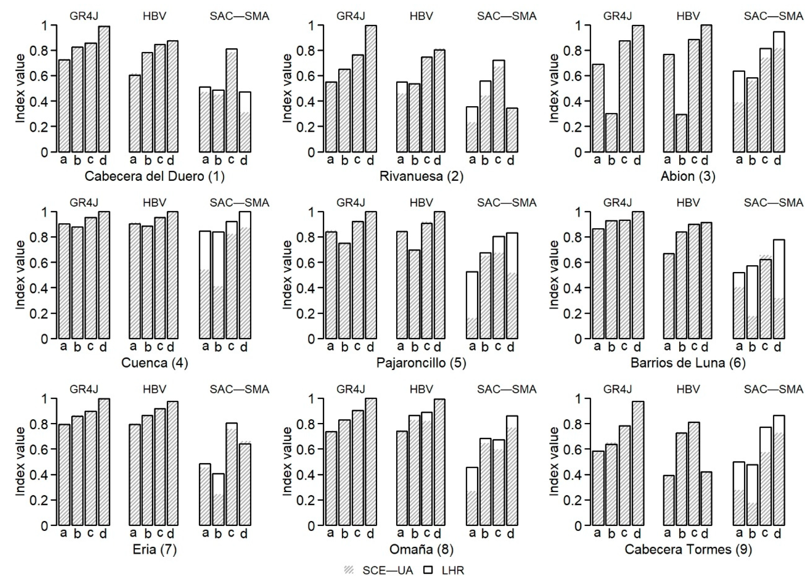
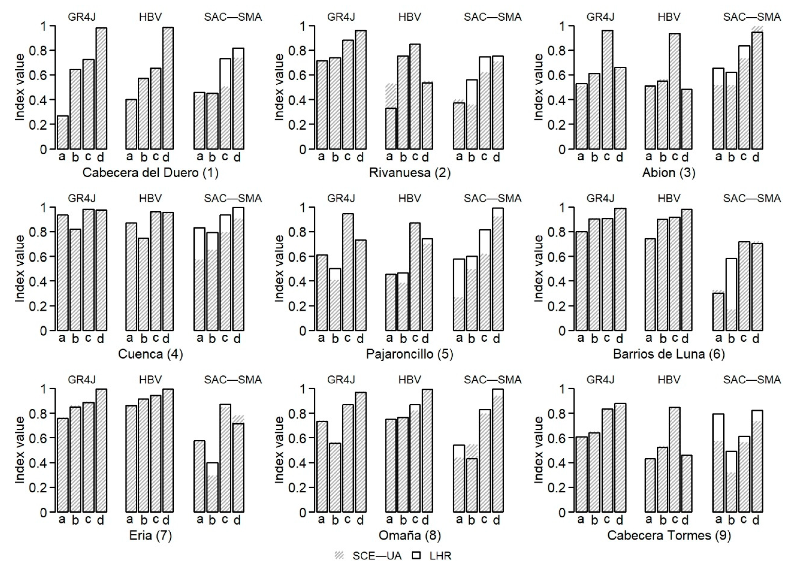
3.2. Comparison of the OF Values

The OF value reached by an algorithm allows evaluation of the quality of a solution and comparing it to others found by different methods to solve the same problem. In this case, we compared the OF values reached by the LHR with the SCE-UA algorithm as a benchmark. Figure 4 shows the median OF values obtained from the calibration stage (for each case-study by hydrological model and for both algorithms), whereas Figure 5 shows the results for the validation stage.
Figure 4 shows that the median OF values achieved by both algorithms during the calibration stage are generally the same in all the study cases for GR4J and HBV. Furthermore, the differences in the OF values for the SAC–SMA model are significant, because the LHR found better OF values than the SCE-UA in the nine study cases. Thus, the variability of the series is better represented by the set of parameters found by the LHR algorithm that that of the SCE-UA. The analysis of the differences in the set of parameters found by both algorithms is shown in Section 3.3.
The calibrations of the nine case studies and the three CRRMs were ‘very good’ or ‘good’, according to [96], except in some cases of SAC-SMA, where the calibration was ‘satisfactory’. There, lower values of the indices were obtained for the rest of the catchments. We attribute this mainly to the complexity of the model. However, it was the best calibration achieved with the conditions established to evaluate the performance of both algorithms under the same circumstances. Moreover, the results from the validation stage are shown in Figure 5 to demonstrate the capacity of the models to represent the processes present in the basins. Generally, we observed that the OF values in the validation stage were satisfactory for both algorithms. In basins 2 and 8, the results from SCE-UA were slightly better than the results from LHR.
An analysis of algorithm efficiency was also performed when a perturbation in the initial parameters of the CRRM was added. According to [85], this is an important characteristic in the calibration stage. Thus, it was concluded that perturbations in the initial CRRM parameter values did not influence the OF value achieved by the algorithms.

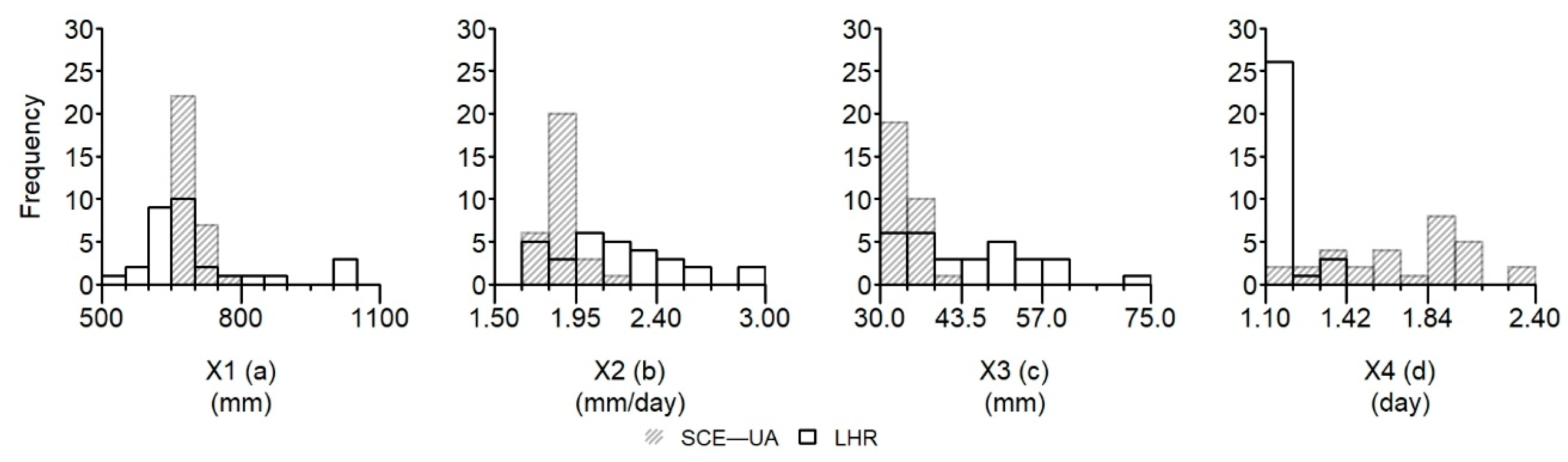
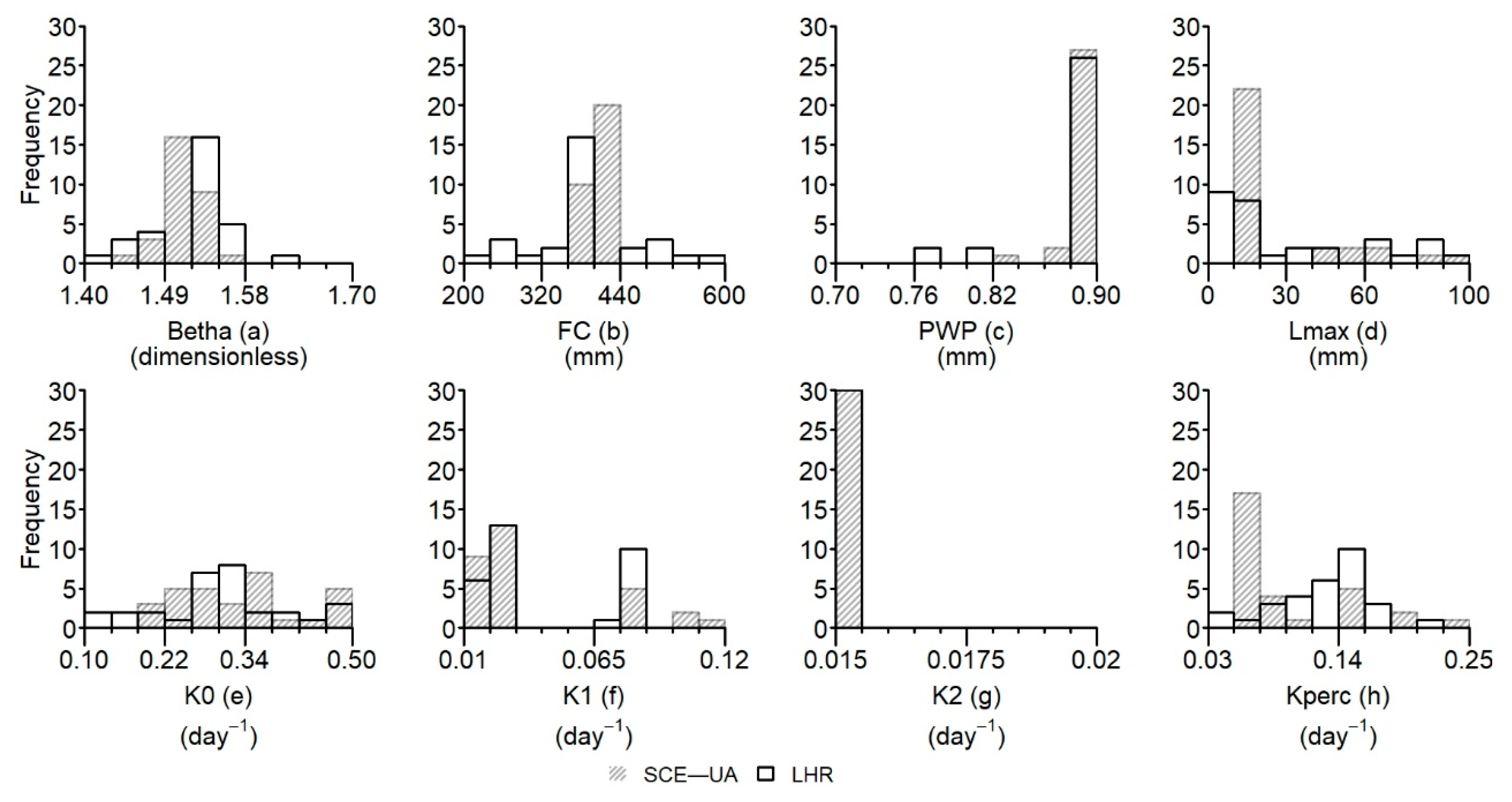
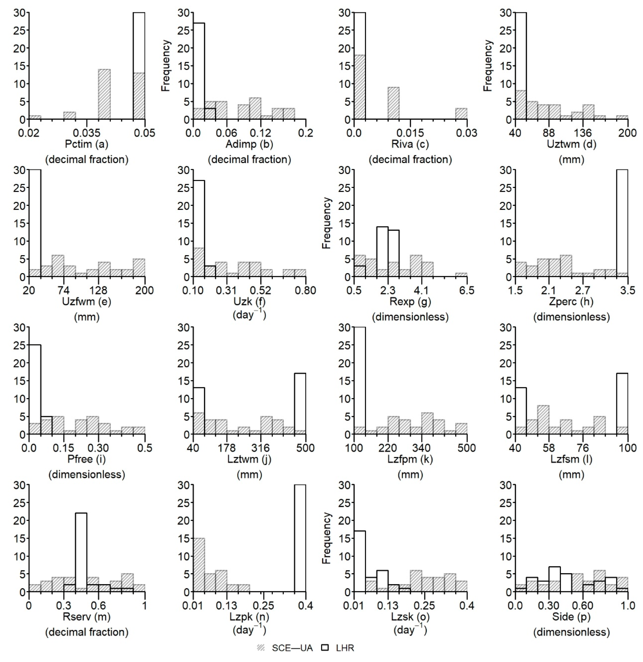
3.3. Comparison of the Effective Parameter Values

Rarely is there a single solution for a specific problem. ‘Equifinality’ of parameter sets is a concept introduced by [97] and [98], who formulated that many different parameter combinations gave an acceptable solution of the same problem. Thus, model simulations should be analysed to generate a set of confidence parameter into a range determined by the model.
To establish the valid range of the parameter values for each model, we launched 30 simulations for each CRRM and basin with both algorithms. Thus, we considered the randomness of the calibration process and each algorithm when searching the optimal solution from different initial points in the sample space. If the algorithm converged at the same set of parameters many times from different points (seeds), it indicates that it could be an optimal parameter set.
Figure 6, Figure 7 and Figure 8 show the optimal solutions found by each algorithm for basin number 5. This analysis was performed for the nine case studies. However, the most representative case is shown below.
The snow parameter values for the four basins are given in Appendix A Table A2. Note that, in the calibration process described in this paper, the snow parameter was set. The parameters were calibrated independently of the 30 simulations for each model, and the snow component was considered an independent variable of the rest of the parameters. Therefore, we reduced the dimensionality of the calibration problem and tested the algorithms homogeneously in all cases.
In the histograms of Figure 6 and Figure 7 (GR4J and HBV, respectively), we observed that the variability of the solutions found by the LHR algorithm is more widespread than that found by the SCE-UA. However, there are also cases where LHR found parameter solutions with minor variations from the benchmark algorithm (Figure 6d). We found cases where the parameter variation was concentrated in a very short range for 30 repetitions with both algorithms (Figure 7g).
However, for all the parameter of the GR4J and HBV models, the 30 repetitions were concentred in similar ranges with different frequencies. Thus, whereas the mathematical formulation was different in both methods, the variability was represented similarly by the algorithms.
Overall, the solutions found by both algorithms were different in the three CRRMs. However, in the results for the SAC-SMA model, the parameters had significant differences. The LHR algorithm had less dispersion in the solutions from the 30 simulations than did the SCE-UA for the nine study cases.
Figure 8 shows the frequency histogram of the solutions found by the algorithms in the calibration for the SAC-SMA model. It is clear that in most of the parameters, the variability found by the LHR algorithm was less than that obtained by solutions with SCE-UA. The LHR plotted 30 repetitions within a unique range, and there have been cases where it was not possible to identify the range of valid solutions using the SCE-UA algorithm (Figure 8i). This behaviour was observed in at least 10 of the 16 parameters calibrated in the SAC-SMA model. Similar conclusions to those described in this section were obtained for the other eight.
The ranges plotted in Figure 6, Figure 7 and Figure 8 represent the range where the algorithms found solutions, not the total search range of the algorithm, which is given in the Appendix A Table A1.

3.4. Comparison of GR4J, HBV and SAC-SMA Performance

This analysis was performed to compare the behaviour of different CRRMs in the simulation of flows in the same catchment. One may note that in many cases GR4J outperforms HBV and SAC-SMA. This variability in the behavior of the models was also found in studies such as [99], relating this performance also to the basin areas.
According to the index values in Figure 5, the GR4J model is capable of better simulating the low flows in the series, because the value obtained from the ln NSE index is almost always slightly higher. The HBV model reflects a high ability to simulate high values better than low flows, because the NSE index has better values than does ln NSE. We also identified that the GR4J model had a higher capacity to simulate the flows following an extreme rainfall event. Regarding the SAC-SMA model, it behaved satisfactorily in all the catchments but has not proved to be the best in any of the cases. This again may be caused by the number of model parameters. Such differences in results are not surprising, because, over a decade ago, [100] showed that various CRRMs performed very differently for different catchments, even those located in zones with similar climatic conditions [101].

3.5. Comparison of the Estimated Runoffs for the Calibration and Validation Periods

Figure 9 and Figure 10 show the calibration and validation plots per month for catchment 5, respectively. The results were analysed for each case-study, using the effective parameter values selected in the previous section. We compared the observed flows for each basin with the simulated flows estimated from the effective parameters for the validation and calibration stages. Generally, the scenario with the least capacity to simulate the measured flows is the SAC-SMA model calibrated with the SCE-UA algorithm. It is observed that, for months where flows were high, this scenario overestimated values and, when flows were low, it did not have the capacity to represent them. The wrong interpretation of the flows measured by this model can also be verified in the OF values calculated in Section 3.2. However, when a comparison is made between the scenario of this model but calibrated with the LHR algorithm, better performance was observed over the previous scenario in both low and high flows. GR4J and HBV represented the variability of measured flows in nearly every month independently of the algorithm used to calibrate the model. These results could be verified with the validation results (Figure 10). Similar conclusions were obtained for the other eight case studies.

3.6. Sensitivity Analysis of the Parameters of the LHR Algorithm

One of the fundamental problems in the application of optimization algorithms in the calibration of CRRMs consists of the determination of a correct and effective set of parameters to search the OF in a reliable and efficient way [102]. A sensitivity analysis of the parameters of the LHR algorithm was conducted to determine their impact on the search for the OF.
The influence evaluation of each parameter on the OF calculation was analysed using 80 combinations of different parameter sets. Each parameter was attempted with variations between the permissible ranges. In each simulation, a unique parameter was variated, whereas the rest retained the main value. The analysis was performed for nine catchments. Figure 11 shows the most representative cases of this analysis.
The ALPHA parameter was analysed in a range of values between 0.5 and 10. Figure 11 shows that, for very high values of ALPHA (from 7.5–10), high OF values were obtained with a high number of iterations. According to previous analyses, this translates into a higher consumption of time. However, it can be observed that, for very low values of ALPHA (from 0.5–3.5), high OF values are reached. In this last range, the OF evaluation number is lower. For average ALPHA values (from 3.5–7.5), the number of iterations is not very high, but the OF value reached is lower than in the previous intervals. The study [31] suggested that this parameter had a value of around 3.0. Based on the sensitivity analysis specifically performed for an ALPHA value equal to 3.0, a high OF value, (no the highest of all analyses, but acceptable) and a very low number of iterations (the second lowest of all analyses) was achieved.
Similarly, the BETA parameter was analysed in a range from −0.9–0.1. According to [31], the suggested value for this parameter was −0.3. The significant differences shown with the variation of this parameter are reflected in the iterations number, rather than in the OF value reached, because the latter remains more or less constant according to Figure 11. For values between −0.9 and −0.6, the number of iterations increased considerably, and the OF value varied by less than 0.01. For values between −0.5 and −0.1, the number of iterations decreased considerably, whereas the OF value reached remained about the same, except for two cases. In the analysis, it was determined that the most suitable value for BETA was −0.3, requiring a low number of iterations for reaching a high OF value.
The number of RNB launches was determined by RLAUNCH. There is a directly proportional relationship between this parameter and the number of iterations. The higher the number of launches, the greater number of iterations. According to Figure 11, it can be established that for RLAUNCH values from 3–5, we get the same OF value, with a different number of iterations. For RLAUNCH values greater than 5, the number of iterations increases considerably, but the improvement in the OF value achieved does not. For RLAUNCH values less than 1 and 2, the number of iterations was smaller but the OF value reached was very low. This determines that the appropriated value of RLAUNCH is equal to 3 in cases of WRA.
LHDIV represents the LH size for initial random sampling. Based on Figure 11, for divisions of LH between 40 and 50, the number of iterations was the lowest of all analyses, and the OF value achieved was among the highest recorded values. For greater LHDIV, the OF evaluation number increased considerably, and the OF value obtained was not necessarily the best. Therefore, the value of the selected LHDIV parameter was 50.
The graph of Figure 11 (corresponding to the STEPROS parameter) shows that the lowest number of iterations evaluations is found for a STEPROS equal to 40, whereas the highest OF values are found for values between 5.0 and 30. However, the number of iterations increases. For values greater than 45 to 100, the number of iterations decreased, compared to the previous interval. Still, the OF value is not the best. It has been suggested to use parameter values between 40 and 80.
MAXN and ERR are the stop criteria of the algorithm, determined according to the dimension of the problem to ensure that these do not affect the calculation of the optimal solution.
This analysis allowed determination of the effective parameters of the LHR algorithm for its application in the solution of problems in the calibration of CRRMs for the evaluation of water resources shown in Table 2. These parameters are used in the calibration of models used in Section 3.5.

4. Conclusions

In this study, a traditional local-search algorithm coupled with a random sampling method as a designer and optimizer of a multi-start strategy was tested. The combination was compared to an evolutionary algorithm for the calibration of three CRRMs with different complexities (HBV, GR4J and SAC-SMA) for nine headwater basins located in potential drought areas of Spain, with different climatic conditions for the WRA.
We observed that the combination of the local search algorithm, RNB, coupled with an efficient random sampling method, LH, which allows prior inspection and evaluation of the launch points of the RNB algorithm, works efficiently in the estimation of the optimal parameters of different CRRMs. When comparing the results of the LHR algorithm with those obtained by the evolutionary algorithm, SCE-UA, we observed that, for models with high complexities, such as the SAC-SMA model, the LHR algorithm found significantly better solutions than the SCE-UA, an algorithm widely used in the solution of this type of problems. For models like GR4J and HBV, having relatively inferior complexities than those of SAC-SMA, the algorithm achieved solutions at least equal to those found by the reference algorithm.
We joined the conclusions of studies of [6,16,17,19], in which it was argued that algorithms catalogued as traditional or historical, could work efficiently to solve actual problems if they are used correctly. The evaluation of the behaviour of a local-search algorithm improved with the random sampling method, in the calibration of the main rainfall–runoff models used in the WRA, was considered. Surprisingly, this algorithm gave positive results and, in the nine cases of the SAC-SMA model, LHR was the best.
It was also observed that the selection of the type of model for simulation of flows in a basin played an important role, because the same model can behave very differently in each case. In fact, the complexity of hydrological models affected the results obtained, depending on the optimization technique selected. Finally, we confirmed that for a flow simulation with a given model, distinct optimization methods perform differently for different catchments. Hence, it is recommended that a series of repetitive tests with different starting values of parameters by each optimization method be undertaken for deciding the most appropriate optimization method. In this case, after a sensitivity analysis of parameters of the LHR algorithm, it was possible to establish the set of optimal values to use for the calibration of CRRMs.

Author Contributions

This manuscript is a result of the Doctoral research of L.G.-R. Formal analysis, L.G.-R.; Investigation, L.G.-R.; Methodology, J.P.-A. and E.B.; Supervision, J.P.-A.; Writing—original draft, L.G.-R.; Writing—review and editing, A.S., J.A. and S.T.S.-Q.

Funding

This research received no external funding.

Acknowledgments

The authors wish to thank the Spanish Research Agency (MINECO) for the financial support to ERAS project (CTM2016-77804-P, including EU-FEDER funds). Additionally, we also value the support provided by the European Community in financing the project IMPREX (H2020-WATER-2014–2015, 641811). The first author would like to express her gratitude to the National Council of Science and Technology of Mexico (CONACyT) for financial support for her Ph.D. studies.

Conflicts of Interest

The authors declare no conflict of interest.

Appendix A

Table A1. Description of the parameters for each CRRM and ranges for the optimization algorithms.
TypeParameter (Units)DescriptionMin.Max.
GR4J
X1 (mm)Maximum capacity of the production store1001200
X2 (mm/day)Groundwater exchange coefficient −53
X3 (mm)One day ahead maximum capacity of the routing store20300
X4 (days)Time base of unit hydrograph UH10.55.8
HBV
Soil parametersBetha (dimensionless)Shape coefficient of recharge function16
FC (mm)Maximum water storage in the unsaturated zone store30650
PWP (mm)Soil moisture value above which actual evaporation reaches potential evaporation30650
Groundwater near the surface parametersLmax (mm)Threshold parameter for extra outflow from upper zone0100
K0 (day−1)Additional recession coefficient of upper groundwater store0.0011
K1 (day−1)Recession coefficient of upper groundwater store0.0011
Deep groundwater parametersK2 (day−1)Recession coefficient of lower groundwater store0.0011
Kperc (mm d−1)Maximum percolation to lower zone0.0011
Snow
parameters
TT (°C)Threshold temperature−1.52.5
DD (mm °C−1 day−1)Degree-day factor030
SAC-SMA
Surface parametersPCTIM (decimal fraction)Impervious fraction of the watershed area 00.1
ADIMP (decimal fraction)Additional impervious area (decimal fraction)00.5
RIVA (decimal fraction)Riparian vegetation area 00.2
Soil parametersUZTWM (mm)Upper zone tension water maximum storage 10500
UZFWM (mm)Upper zone free water maximum storage 10500
UZK (day−1)Upper zone free water lateral depletion rate 0.10.9
REXP (dimensionless)Exponent of the percolation equation 15
ZPERC (dimensionless)Maximum percolation rate 1250
Groundwater parametersPFREE (decimal fraction)Fraction of water percolating from upper zone directly to lower zone free water storage 00.9
LZTWM (mm)Lower zone tension water maximum storage 5700
LZFPM (mm)Lower zone free water primary maximum storage 5500
LZFSM (mm)Lower zone free water supplemental maximum storage 5500
RSERV (decimal fraction)Fraction of lower zone free water not transferrable to lower zone tension water 10.9
LZPK (day−1)Lower zone primary free water depletion rate 0.00010.6
Table A2. Snow parameter values resulting from the independent calibration process for the basins with snow influence.
Case-Study CatchmentsThreshold Temperature
TT
(°C)
Degree-Day Factor DD
(mm °C−1 Day−1)
6010.05
7011.72
804.49
9015.22

References

  1. Bellin, A.; Majone, B.; Cainelli, O.; Alberici, D.; Villa, F. A continuous coupled hydrological and water resources management model. Environ. Model. Softw. 2016, 75, 176–192. [Google Scholar] [CrossRef]
  2. Arsenault, R.; Poulin, A.; Côté, P.; Brissette, F. Comparison of Stochastic Optimization Algorithms in Hydrological Model Calibration. J. Hydrol. Eng. 2014, 19, 1374–1384. [Google Scholar] [CrossRef]
  3. Abdulla, F.; Al-Badranih, L. Application of a rainfall-runoff model to three catchments in Iraq. Hydrol. Sci. J. 2000, 45, 13–25. [Google Scholar] [CrossRef]
  4. Devi, G.K.; Ganasri, B.P.; Dwarakish, G.S. A Review on Hydrological Models. Aquat. Procedia 2015, 4, 1001–1007. [Google Scholar] [CrossRef]
  5. Coron, L.; Thirel, G.; Delaigue, O.; Perrin, C.; Andréassian, V. The suite of lumped GR hydrological models in an R package. Environ. Model. Softw. 2017, 94, 166–171. [Google Scholar] [CrossRef]
  6. Chlumecký, M.; Buchtele, J.; Richta, K. Application of random number generators in genetic algorithms to improve rainfall-runoff modelling. J. Hydrol. 2017, 553, 350–355. [Google Scholar] [CrossRef]
  7. Laloy, E.; Vrugt, J.A. High-dimensional posterior exploration of hydrologic models using multiple-try DREAM (ZS) and high-performance computing. Water Resour. Res. 2012, 48, 1–18. [Google Scholar] [CrossRef]
  8. Chu, W.; Gao, X.; Sorooshian, S. Improving the shuffled complex evolution scheme for optimization of complex nonlinear hydrological systems: Application to the calibration of the Sacramento soil-moisture accounting model. Water Resour. Res. 2010, 46, 1–12. [Google Scholar] [CrossRef]
  9. Duan, Q.; Sorooshian, S.; Gupta, V.K. Effective and Efficient Global Optimization for Conceptual Rainfall-Runoff Models. Water Resour. Res. 1992, 28, 1015–1031. [Google Scholar] [CrossRef]
  10. Jiang, Y.; Li, X.; Huang, C. Automatic calibration a hydrological model using a master-slave swarms shuffling evolution algorithm based on self-adaptive particle swarm optimization. Expert Syst. Appl. 2013, 40, 752–757. [Google Scholar] [CrossRef]
  11. Kim, S.M.; Benham, B.L.; Brannan, K.M.; Zeckoski, R.W.; Doherty, J. Comparison of hydrologic calibration of HSPF using automatic and manual methods. Water Resour. Res. 2007, 43, 1–12. [Google Scholar] [CrossRef]
  12. Willems, P.; Mora, D.; Vansteenkiste, T.; Taye, M.T.; Van Steenbergen, N. Parsimonious rainfall-runoff model construction supported by time series processing and validation of hydrological extremes—Part 2: Intercomparison of models and calibration approaches. J. Hydrol. 2014, 510, 591–609. [Google Scholar] [CrossRef]
  13. Vansteenkiste, T.; Tavakoli, M.; Van Steenbergen, N.; De Smedt, F.; Batelaan, O.; Pereira, F.; Willems, P. Intercomparison of five lumped and distributed models for catchment runoff and extreme flow simulation. J. Hydrol. 2014, 511, 335–349. [Google Scholar] [CrossRef]
  14. Tolson, B.A.; Shoemaker, C.A. Dynamically dimensioned search algorithm for computationally efficient watershed model calibration. Water Resour. Res. 2007, 43, 1–16. [Google Scholar] [CrossRef]
  15. Moradkhani, H.; Sorooshian, S. General review of rainfall-runoff modeling: Model calibration, data assimilation, and uncertainty analysis. In Hydrological Modelling and the Water Cycle. Water Science and Technology Library; Sorooshian, S., Hsu, K., Coppola, E., Tomassetti, B., Verdecchia, M., Visconti, G., Eds.; Springer: Berlin/Heidelberg, Germany, 2009; Volume 63, ISBN 978-3-540-77843-1. [Google Scholar]
  16. Piotrowski, A.P.; Napiorkowski, M.J.; Napiorkowski, J.J.; Osuch, M.; Kundzewicz, Z.W. Are modern metaheuristics successful in calibrating simple conceptual rainfall-runoff models? Hydrol. Sci. J. 2017, 62, 606–625. [Google Scholar] [CrossRef]
  17. Piotrowski, A.P.; Napiorkowski, M.J.; Napiorkowski, J.J.; Rowinski, P.M. Swarm Intelligence and Evolutionary Algorithms: Performance versus speed. Inf. Sci. 2017, 384, 34–85. [Google Scholar] [CrossRef]
  18. Goswami, M.; O’Connor, K.M. Comparative assessment of six automatic optimization techniques for calibration of a conceptual rainfall-runoff model. Hydrol. Sci. J. 2007, 52, 432–449. [Google Scholar] [CrossRef]
  19. Piotrowski, A.P.; Napiorkowski, J.J.; Osuch, M. Relationship Between Calibration Time and Final Performance of Conceptual Rainfall-Runoff Models. Water Resour. Manag. 2018, 1–19. [Google Scholar] [CrossRef]
  20. Sörensen, K. Metaheuristics-the metaphor exposed. Int. Trans. Oper. Res. 2015, 22, 3–18. [Google Scholar] [CrossRef]
  21. Maier, H.R.; Kapelan, Z.; Kasprzyk, J.; Kollat, J.B.; Matott, L.S.; Cunha, M.C.; Dandy, G.C.; Gibbs, M.S.; Keedwell, E.; Marchi, A.; et al. Evolutionary algorithms and other metaheuristics in water resources: Current status, research challenges and future directions. Environ. Model. Softw. 2014, 62, 271–299. [Google Scholar] [CrossRef] [Green Version]
  22. Piotrowski, A.P. Regarding the rankings of optimization heuristics based on artificially-constructed benchmark functions. Inf. Sci. 2015, 297, 191–201. [Google Scholar] [CrossRef]
  23. Reed, P.M.; Hadka, D.; Herman, J.D.; Kasprzyk, J.R.; Kollat, J.B. Evolutionary multiobjective optimization in water resources: The past, present, and future. Adv. Water Resour. 2013, 51, 438–456. [Google Scholar] [CrossRef]
  24. Thyer, M.; Kuczera, G.; Bates, B.C. Probabilistic optimization for conceptual rainfall-runoff models: A comparison of the shuffled complex evolution and simulated annealing algorithms. Water Resour. Res. 1999, 35, 767–773. [Google Scholar] [CrossRef] [Green Version]
  25. Azamathulla, H.M.; Wu, F.-C.; Ghani, A.A.; Narulkar, S.M.; Zakaria, N.A.; Chang, C.K. Comparison between genetic algorithm and linear programming approach for real time operation. J. Hydro Environ. Res. 2008, 2, 172–181. [Google Scholar] [CrossRef]
  26. Franchini, M.; Galeati, G. Comparing several genetic algorithm schemes for the calibration of conceptual rainfall-runoff models. Hydrol. Sci. J. 1997, 42, 357–380. [Google Scholar] [CrossRef]
  27. Hendrickson, J.D.; Sorooshian, S.; Brazil, L.E. Comparison of Newton-Type and Direct Search Algorithms for Calibration Rainfall-Runoff Models. Water Resour. Res. 1988, 24, 691–700. [Google Scholar] [CrossRef]
  28. Huang, X.; Liao, W.; Lei, X.; Jia, Y.; Wang, Y.; Wang, X.; Jiang, Y.; Wang, H. Parameter optimization of distributed hydrological model with a modified dynamically dimensioned search algorithm. Environ. Model. Softw. 2014, 52, 98–110. [Google Scholar] [CrossRef]
  29. Kollat, J.B.; Reed, P.M. Comparing state-of-the-art evolutionary multi-objective algorithms for long-term groundwater monitoring design. Adv. Water Resour. 2006, 29, 792–807. [Google Scholar] [CrossRef]
  30. Lerma, N.; Paredes-Arquiola, J.; Andreu, J.; Solera, A.; Sechi, G.M. Assessment of evolutionary algorithms for optimal operating rules design in real Water Resource Systems. Environ. Model. Softw. 2015, 69, 425–436. [Google Scholar] [CrossRef]
  31. Rosenbrock, H.H. An Automatic Method for finding the Greatest or Least Value of a Function. Comput. J. 1960, 3, 175–184. [Google Scholar] [CrossRef]
  32. Ibbitt, R.P.; O’Donnell, T. Fitting Methods for Conceptual Catchments Models. J. Hydraul. Div. 1971, 97, 1341–1342. [Google Scholar]
  33. Kachroo, R.K.; Sea, C.H.; Warsi, M.S.; Jemenez, H.; Saxena, R.P. River flow forecasting. Part 3. Applications of linear techniques in modelling rainfall-runoff transformations. J. Hydrol. 1992, 133, 41–97. [Google Scholar] [CrossRef]
  34. Liang, G.; Kachroo, R.; Kang, W.; Yu, X. River flow forecasting. Part 4. Applications of linear modelling techniques for flow routing on large catchments. J. Hydrol. 1992, 133, 98–140. [Google Scholar] [CrossRef]
  35. Price, W.L. A controlled random search procedure for global optimisation. Comput. J. 1977, 20, 367–370. [Google Scholar] [CrossRef] [Green Version]
  36. Masri, S.G.; Bekey, G.A.; Safford, F.B. A global optimization algorithm using adaptive random search. Appl. Math. Comput. 1980, 7, 353–375. [Google Scholar] [CrossRef]
  37. Pronzato, L.; Walter, E.; Venot, A.; Lebruchec, J.-F. A general-purpose global optimizer: Implimentation and applications. Math. Comput. Simul. 1984, 26, 412–422. [Google Scholar] [CrossRef]
  38. Spendley, W.; Hext, G.R.; Himsworth, F.R. Sequential Application of Simplex Designs in Optimisation and Evolutionary Operation. Technometrics 1962, 4, 441–461. [Google Scholar] [CrossRef]
  39. Nelder, J.A.; Mead, R. A Simplex Method for Function Minimization. Comput. J. 1965, 7, 308–313. [Google Scholar] [CrossRef]
  40. Hooke, R.; Jeeves, T.A. “Direct Search” Solution of Numerical and Statistical Problems. J. ACM 1961, 8, 212–229. [Google Scholar] [CrossRef]
  41. Muttil, N.; Jayawardena, A.W. Shuffled Complex Evolution model calibrating algorithm: Enhancing its robustness and efficiency. Hydrol. Process. 2008, 22, 4628–4638. [Google Scholar] [CrossRef]
  42. Franchini, M.; Galeati, G.; Berra, S. Global optimization techniques for the calibration of conceptual rainfall-runoff models. Hydrol. Sci. J. 1998, 43, 443–458. [Google Scholar] [CrossRef]
  43. Poikolainen, I.; Neri, F.; Caraffini, F. Cluster-Based Population Initialization for differential evolution frameworks. Inf. Sci. 2015, 297, 216–235. [Google Scholar] [CrossRef] [Green Version]
  44. Kolda, T.G.; Lewis, R.M.; Torczon, V. Optimization by Direct Search: New Perspectives on Some Classical and Modern Methods. Soc. Ind. Appl. Math. 2003, 45, 385–482. [Google Scholar] [CrossRef]
  45. Chau, K. Use of meta-heuristic techniques in rainfall-runoff modelling. Water (Switz.) 2017, 9, 186. [Google Scholar] [CrossRef]
  46. Crepinsek, M.; Liu, S.-H.; Mernik, M. Exploration and Exploitation in Evolutionary Algorithms: A Survey. ACM Comput. Surv. Artic. 2013, 45, 1–33. [Google Scholar] [CrossRef]
  47. Weyland, D. A Rigorous Analysis of the Harmony Search Algorithm: How the Research Community can be Misled by a “Novel” Methodology. Int. J. Appl. Metaheuristic Comput. 2010, 1, 50–60. [Google Scholar] [CrossRef]
  48. Cooper, V.A.; Nguyen, V.T.V.; Nicell, J.A. Calibration of conceptual rainfall-runoff models using global optimisation methods with hydrologic process-based parameter constraints. J. Hydrol. 2007, 334, 455–466. [Google Scholar] [CrossRef]
  49. Kuczera, G. Efficient subspace probabilistic parameter optimization for catchment models. Water Resour. Res. 1997, 33, 177–185. [Google Scholar] [CrossRef]
  50. Gan, T.Y.; Biftu, G.F. Automatic calibration of conceptual rainfall-runoff models: Optimization algorithms, catchment conditions, and model structure. Water Resour. Res. 1996, 32, 3513–3524. [Google Scholar] [CrossRef]
  51. Sorooshian, S.; Duan, Q.; Gupta, V.K. Calibration of Rainfall-Runoff Models: Application of Global Optimization to the Sacramento Soil Moisture Accounting Model. Water Resour. Res. 1993, 29, 1185–1194. [Google Scholar] [CrossRef]
  52. Abdulla, F.A.; Lettenmaier, D.P.; Liang, X. Estimation of the ARNO model baseflow parameters using daily streamflow data. J. Hydrol. 1999, 222, 37–54. [Google Scholar] [CrossRef]
  53. Franchini, M. Use of a genetic algorithm combined with a local search method for the automatic calibration of conceptual rainfall-runoff models. Hydrol. Sci. J. 1996, 41, 21–39. [Google Scholar] [CrossRef]
  54. Dakhlaoui, H.; Bargaoui, Z.; Bárdossy, A. Toward a more efficient Calibration Schema for HBV rainfall-runoff model. J. Hydrol. 2012, 444–445, 161–179. [Google Scholar] [CrossRef]
  55. Granata, F.; Gargano, R.; de Marinis, G. Support vector regression for rainfall-runoffmodeling in urban drainage: A comparison with the EPA’s storm water management model. Water (Switz.) 2016, 8, 69. [Google Scholar]
  56. Onyutha, C. Hydrological model supported by a step-wise calibration against sub-flows and validation of extreme flow events. Water (Switz.) 2019, 11, 244. [Google Scholar] [CrossRef]
  57. Haro-Monteagudo, D.; Solera, A.; Andreu, J. Drought early warning based on optimal risk forecasts in regulated river systems: Application to the Jucar River Basin (Spain). J. Hydrol. 2017, 544, 36–45. [Google Scholar] [CrossRef]
  58. Madrigal, J.; Solera, A.; Suárez-Almiñana, S.; Paredes-Arquiola, J.; Andreu, J.; Sánchez-Quispe, S.T. Skill assessment of a seasonal forecast model to predict drought events for water resource systems. J. Hydrol. 2018, 564, 574–587. [Google Scholar] [CrossRef]
  59. Morán-Tejeda, E.; Ceballos-Barbancho, A.; Llorente-Pinto, J.M. Hydrological response of Mediterranean headwaters to climate oscillations and land-cover changes: The mountains of Duero River basin (Central Spain). Glob. Planet. Chang. 2010, 72, 39–49. [Google Scholar] [CrossRef]
  60. Kahil, M.T.; Albiac, J.; Dinar, A.; Calvo, E.; Esteban, E.; Avella, L.; Garcia-Molla, M. Improving the performance of water policies: Evidence from drought in Spain. Water (Switz.) 2016, 8, 34. [Google Scholar] [CrossRef]
  61. Fayad, A.; Gascoin, S.; Faour, G.; López-Moreno, J.I.; Drapeau, L.; Le Page, M.; Escadafal, R. Snow hydrology in Mediterranean mountain regions: A review. J. Hydrol. 2017, 551, 374–396. [Google Scholar] [CrossRef]
  62. Herrera, S.; Gutiérrez, J.M.; Ancell, R.; Pons, M.R.; Frías, M.D.; Fernández, J. Development and analysis of a 50-year high-resolution daily gridded precipitation dataset over Spain (Spain02). Int. J. Climatol. 2012, 32, 74–85. [Google Scholar] [CrossRef]
  63. Hargreaves, G.H.; Samani, Z.A. Reference crop evapotranspiration from temperature. Appl. Eng. Agric. 1985, 1, 96–99. [Google Scholar] [CrossRef]
  64. MAPAMA—Ministerio de Agricultura y Pesca, Alimentación y Medio Ambiente. Sistema de Información del Anuario de Aforos. (2013–2014). Available online: http://ceh-flumen64.cedex.es/anuarioaforos/default.asp (accessed on 15 March 2019).
  65. Garcia, F.; Folton, N.; Oudin, L. Which objective function to calibrate rainfall–runoff models for low-flow index simulations? Hydrol. Sci. J. 2017, 62, 1149–1166. [Google Scholar] [CrossRef]
  66. Oudin, L.; Andréassian, V.; Mathevet, T.; Perrin, C.; Michel, C. Dynamic averaging of rainfall-runoff model simulations from complementary model parameterizations. Water Resour. Res. 2006, 42, 1–10. [Google Scholar] [CrossRef]
  67. Madsen, H. Automatic calibration of a conceptual rainfall–runoff model using multiple objectives. J. Hydrol. 2000, 235, 276–288. [Google Scholar] [CrossRef]
  68. Yapo, P.O.; Gupta, H.V.; Sorooshian, S. Automatic calibration of conceptual rainfall-runoff models: Sensitivity to calibration data. J. Hydrol. 1996, 181, 23–48. [Google Scholar] [CrossRef]
  69. Bergström, S.; Harlin, J.; Lindström, G. Spillway design floods in Sweden: I. New guidelines. Hydrol. Sci. J. 1992, 37, 505–519. [Google Scholar] [CrossRef] [Green Version]
  70. Bergström, S. The HBV Model. In Computer Models of Watershed Hydrology; Singh, V.P., Ed.; Water Resources Publications: Highlands Ranch, CO, USA, 1995; pp. 443–476. [Google Scholar]
  71. Burnash, R.J.C.; Ferral, R.L.; McGuire, R.A. A Generalized Streamflow Simulation System-Conceptual Modeling for Digital Computers; Technical Report; United States Department of Commerce, National Weather Service and State of California, Department of Water Resources: Sacramento, CA, USA, 1973; p. 204. [Google Scholar]
  72. Perrin, C.; Michel, C.; Andréassian, V. Improvement of a parsimonious model for streamflow simulation. J. Hydrol. 2003, 279, 275–289. [Google Scholar] [CrossRef]
  73. Paredes-Arquiola, J.; Lerma, N.; Solera, A.; Andreu, J. Herramienta EvalHid Para la Evaluación de Recursos Hídricos. Manual de Usuario v1.1; Departamento de Ingeniería del Agua y Medioambiental, Grupo de Ingeniería de Recursos Hídricos, Universitat Politència de València: Valencia, Spain, 2017. (In Spanish) [Google Scholar]
  74. Ficchì, A.; Perrin, C.; Andréassian, V. Impact of temporal resolution of inputs on hydrological model performance: An analysis based on 2400 flood events. J. Hydrol. 2016, 538, 454–470. [Google Scholar] [CrossRef]
  75. Rojas-Serna, C.; Lebecherel, L.; Perrin, C.; Andréassian, V.; Oudin, L. How should a rainfall-runoff model be parameterized in an almost ungauged catchment? A methodology tested on 609 catchments. Water Resour. Res. 2016, 52, 4765–4784. [Google Scholar] [CrossRef] [Green Version]
  76. SMHI. Integrated Hydrological Modelling System (IHMS); Swedish Meteorological and Hydrological Institute: Norrköping, Sweden, 2012. [Google Scholar]
  77. Seibert, J. Regionalisation of parameters for a conceptual rainfall-runoff model. Agric. For. Meteorol. 1999, 98–99, 279–293. [Google Scholar] [CrossRef]
  78. Lindström, G.; Johansson, B.; Persson, M.; Gardelin, M.; Bergström, S. Development and test of the distributed HBV-96 hydrological model. J. Hydrol. 1997, 201, 272–288. [Google Scholar] [CrossRef]
  79. Zhang, G.; Xie, T.; Zhang, L.; Hua, X.; Liu, F. Application of multi-step parameter estimation method based on optimization algorithm in sacramento model. Water (Switz.) 2017, 9, 495. [Google Scholar] [CrossRef]
  80. McKay, M.D.; Beckman, R.J.; Conover, W.J. Comparison of Three Methods for Selecting Values of Input Variables in the Analysis of Output from a Computer Code. Technometrics 1979, 21, 239–245. [Google Scholar]
  81. Muleta, M.K.; Nicklow, J.W. Sensitivity and uncertainty analysis coupled with automatic calibration for a distributed watershed model. J. Hydrol. 2005, 306, 127–145. [Google Scholar] [CrossRef] [Green Version]
  82. Iman, R.L.; Conover, W.J. Small sample sensitivity analysis techniques for computer models with an application to risk assessment. Commun. Stat. Methods 1980, 9, 1749–1842. [Google Scholar] [CrossRef]
  83. Andréassian, V.; Bourgin, F.; Oudin, L.; Mathevet, T.; Perrin, C.; Lerat, J.; Coron, L.; Berthet, L. Seeking genericity in the selection of parameter sets: Impact on hydrological model efficiency. Water Resour. Res. 2014, 48, 8356–8366. [Google Scholar] [CrossRef]
  84. Björck, Å. Numerics of Gram-Schmidt orthogonalization. Linear Algebra Appl. 1994, 197–198, 297–316. [Google Scholar]
  85. Jain, S.K. Calibration of conceptual models for rainfall-runoff simulation. Hydrol. Sci. J. 1993, 38, 431–441. [Google Scholar] [CrossRef]
  86. Duan, Q.; Sorooshian, S.; Gupta, V.K.G. Optimal use of the SCE-UA global optimization method for calibrating watershed models. J. Hydrol. 1994, 158, 265–284. [Google Scholar] [CrossRef]
  87. Duan, Q.Y.; Gupta, V.K.; Sorooshian, S. Shuffled Complex Evolution Approach for Effective and Efficient Global Minimization. J. Optim. Theory Appl. 1993, 76, 501–521. [Google Scholar] [CrossRef]
  88. Janssen, P.H.M.; Heuberger, P.S.C. Calibration of process-oriented models. Ecol. Model. 1995, 83, 55–66. [Google Scholar] [CrossRef]
  89. Cooper, V.A.; Nguyen, V.T.V.; Nicell, J.A. Evaluation of global optimization methods for conceptual rainfall-runoff model calibration. Water Sci. Technol. 1997, 36, 53–60. [Google Scholar] [CrossRef]
  90. Boyle, D.P.; Gupta, H.V.; Sorooshian, S. Toward improved calibration of hydrologic models: Combining the strengths of manual and automatic methods. Water Resour. Res. 2000, 36, 3663–3674. [Google Scholar] [CrossRef]
  91. Nash, J.E.; Sutcliffe, J.V. River Flow Forecasting Through Conceptual Models Part I- A Discussion of Principles. J. Hydrol. 1970, 10, 282–290. [Google Scholar] [CrossRef]
  92. Li, Y.; Ryu, D.; Western, A.W.; Wang, Q.J. Assimilation of stream discharge for flood forecasting: Updating a semidistributed model with an integrated data assimilation scheme. Water Resour. Res. 2015, 51, 3238–3258. [Google Scholar] [CrossRef]
  93. Muleta, M.K. Model Performance Sensitivity to Objective Function during Automated Calibrations. J. Hydrol. Eng. 2012, 17, 756–767. [Google Scholar] [CrossRef]
  94. Pushpalatha, R.; Perrin, C.; Le Moine, N.; Andréassian, V. A review of efficiency criteria suitable for evaluating low-flow simulations. J. Hydrol. 2012, 420–421, 171–182. [Google Scholar] [CrossRef]
  95. Młyński, D.; Petroselli, A.; Wałęga, A. Flood frequency analysis by an event-based rainfall-runoff model in selected catchments of Southern Poland. Soil Water Res. 2018, 13, 170–176. [Google Scholar]
  96. Moriasi, D.N.; Arnold, J.G.; Van Liew, M.W.; Binger, R.L.; Harmel, R.D.; Veith, T.L. Model evaluation guidelines for systematic quantification of accuracy in watershed simulations. Trans. ASABE 2007, 50, 885–900. [Google Scholar] [CrossRef]
  97. Beven, K.; Binley, A. The Future of Distributed Models: Model Calibration and Uncertainty Prediction. Hydrol. Process. 1992, 6, 279–298. [Google Scholar] [CrossRef]
  98. Beven, K. Prophecy, reality and uncertainty in distributed hydrological modelling. Adv. Water Resour. 1993, 16, 41–51. [Google Scholar] [CrossRef]
  99. Li, H.; Xu, C.-Y.; Beldring, S. How much can we gain by increasing degree of model complexity? J. Hydrol. 2015, 527, 858–871. [Google Scholar] [CrossRef]
  100. Perrin, C.; Michel, C.; Andréassian, V. Does a large number of parameters enhance model performance? Comparative assessment of common catchment model structures on 429 catchments. J. Hydrol. 2001, 242, 275–301. [Google Scholar] [CrossRef]
  101. Osuch, M.; Romanowicz, R.J.; Booij, M.J. The influence of parametric uncertainty on the relationships between HBV model parameters and climatic characteristics. Hydrol. Sci. J. 2015, 60, 1299–1316. [Google Scholar] [CrossRef] [Green Version]
  102. Qi, W.; Zhang, C.; Fu, G.; Zhou, H. Quantifying dynamic sensitivity of optimization algorithm parameters to improve hydrological model calibration. J. Hydrol. 2016, 533, 213–223. [Google Scholar] [CrossRef] [Green Version]
Figure 1. Location of the case-study catchments.
Water 11 01876 g001
Figure 2. Joint operation of the Rosenbrock (RNB) algorithm and the method of statistical design of experiments (Latin hypercube, LH). It shows the first RNB launch, where (a) relates the functioning of the LH and (b) indicates the RNB objective.
Water 11 01876 g002
Figure 3. Dispersion and median values in the iteration number required per model type and per algorithm to convergence.
Water 11 01876 g003
Figure 4. Comparison of the median indices’ values used to calculate the objective functions (OF) during the calibration stage for each case-study and for three rainfall–runoff models of different complexities. The figure shows Nash–Sutcliffe efficiency (NSE) (a), ln NSE (log-transformation of the NSE coefficient) (b), r (c) and MS (mean symmetry measure) (d). Every index is the result of the median of 30 simulations in each case-study.
Water 11 01876 g004
Figure 5. Comparison of the median indices’ values used in the validation stage for each case-study and for three rainfall–runoff models with different complexities. The figure shows NSE (a), ln NSE (b), r (c) and MS (d). Every index is the result of the median of 30 simulations of each case-study.
Water 11 01876 g005
Figure 6. Frequency histogram of parameters of the French rural-engineering-with-four-daily-parameters (GR4J) model for basin 5.
Water 11 01876 g006
Figure 7. Frequency histogram of parameters of the Swedish Hydrological Office Water-balance Department (HBV) model for basin 5.
Water 11 01876 g007
Figure 8. Frequency histogram of parameters of the SAC-SMA model for basin 5.
Water 11 01876 g008
Figure 9. Comparison of runoff (average year) obtained from the calibration period for catchment 5 for the three conceptual rainfall–runoff models (CRRMs) and both algorithms.
Water 11 01876 g009
Figure 10. Comparison of runoff (average year) obtained from the validation period for catchment 5 for the three CRRMs and both algorithms.
Water 11 01876 g010
Figure 11. Parameter sensitivity analysis of LHR from 80 algorithm runs.
Water 11 01876 g011
Table 1. Summary information about the case-study catchments.
Case-Study
Catchments
Surface
(km2)
Average Annual
P (mm)
Average Annual
PE (mm)
Average Annual Flow (hm3)Presence of SnowFlow
System
1Cab. del Duero133.1755.8832.993.4NoDuero
2Rivanuesa93.2862.5776.672.3NoDuero
3Abión897.8581.5986.3150.0NoDuero
4Cuenca1005.6601.91057.3300.7NoJúcar
5Pajaroncillo829.0589.81031.3161.3NoJúcar
6Barrios de Luna492.1946.7760.8447.6YesDuero
7Eria283.0744.7858.0153.0YesDuero
8Omaña403.6793.4820.996.1YesDuero
9Cab. del Tormes627.4813.7973.5688.0YesDuero
Table 2. Set of parameter values for the Latin hypercube and Rosenbrock (LHR) method.
NumberParameter NameDescriptionSet Value
1ALPHAAdvance or progress coefficient3
2BETASetback coefficient−0.5
3RLAUNCHRNB launches number3
4LHDIVLH dimension50
5STEPROSRange subdivision parameter40
6ERRIncrement in each time step0.001
7MAXNMaximum number of iterations3000

