Article

Sensitivity of Potential Groundwater Recharge to Projected Climate Change Scenarios: A Site-Specific Study in the Nebraska Sand Hills, USA

1
Department of Earth and Atmospheric Sciences, University of Nebraska-Lincoln, Lincoln NE 68588, USA
2
The World Resources Institute, Washington DC 20002, USA
3
HDR, Omaha, NE 68106, USA
4
Institute of Surface-Earth System Science, Tianjin University, Tianjin 300072, China
5
Department of Agriculture, Division of Agricultural, Forest and Biosystems Engineering, University of Napoli Federico II, Via Università n. 100, 80055 Portici (Napoli), Italy
*
Author to whom correspondence should be addressed.
Water 2019, 11(5), 950; https://doi.org/10.3390/w11050950
Submission received: 5 April 2019 / Revised: 29 April 2019 / Accepted: 30 April 2019 / Published: 6 May 2019
(This article belongs to the Special Issue Water Flow, Solute and Heat Transfer in Groundwater)

Abstract

:
Assessing the relationship between climate forcings and groundwater recharge (GR) rates in semi-arid regions is critical for water resources management. This study presents the impact of climate forecasts on GR within a probabilistic framework in a site-specific study in the Nebraska Sand Hills (NSH), the largest stabilized sand dune region in the USA containing the greatest recharge rates within the High Plains Aquifer. A total of 19 downscaled climate projections were used to evaluate the impact of precipitation and reference evapotranspiration on GR rates simulated by using HYDRUS 1-D. The analysis of the decadal aridity index (AI) indicates that climate class will likely remain similar to the historic average in the RCP2.6, 4.5, and 6.0 emission scenarios but AI will likely decrease significantly under the worst-case emission scenario (RCP8.5). However, GR rates will likely decrease in all of the four emission scenarios. The results show that GR generally decreases by ~25% under the business-as-usual scenario and by nearly 50% in the worst-case scenario. Moreover, the most likely GR values are presented with respect to probabilities in AI and the relationship between annual-average precipitation and GR rate were developed in both historic and projected scenarios. Finally, to present results at sub-annual time resolution, three representative climate projections (dry, mean and wet scenarios) were selected from the statistical distribution of cumulative GR. In the dry scenario, the excessive evapotranspiration demand in the spring and precipitation deficit in the summer can cause the occurrence of wilting points and plant withering due to excessive root-water-stress. This may pose significant threats to the survival of the native grassland ecology in the NSH and potentially lead to desertification processes if climate change is not properly addressed.

Highlights

(1)
Multi-decadal averages of groundwater recharge rates will likely decrease in all emission scenarios despite the region maintaining its historic climate classification as semi-arid.
(2)
In the dry climate scenario analysis, summer is the most sensitive season with a projected reduction in precipitation by 25% and in groundwater recharge rates by 60%.
(3)
The dry climate scenario indicates a notable increase in root water stress and a greater likelihood of desiccation of grass and desertification.

1. Introduction

Socioeconomic drivers have historically determined and will continue to dictate the ever-increasing rate of groundwater depletion around the world. Water consumption in most countries has considerably increased over recent decades due to population and economic growth, with irrigation water use being the leading consumer. In addition to overexploitation, groundwater recharge (GR) regimes are affected by climate change and variability, which threatens environmental sustainability and the livelihoods of billions around the world. The dire water scarcity issues make it imperative to assess the consequences of climate change on water resources at global, continental, and local scales with particular emphasis on GR rates that feed shallow aquifers [1,2,3,4]. Groundwater levels of many aquifers have been showing a decreasing trend over the last few decades due to excessive groundwater extraction for irrigation that surpasses GR and replenishing rates [5,6]. The vulnerability of groundwater resources emphasizes the need for stakeholders and decision-makers to have reliable information regarding the relationship between climate and GR rates, particularly in semi-arid regions where water scarcity issues are well documented [6].
The assessment of climate change can vary in the type of impact, scale, and severity. The negative consequences of climate change in some settings can prove to be pronounced and include severe droughts [7], sea-level rise [8], wildfires [9], extreme heat waves [10], floods and inundation [11], reduction of biodiversity [12], and many others.
The impact of climate change on the water budget in semi-arid regions primarily occurs via changes to potential evapotranspiration (ET) rates and precipitation (P) regime [13]. The rise in temperatures can cause increases in potential ET [14]. Similarly, climate change has been reported to impact the amount and seasonality of P regime [15] which can alter surface runoff and streamflow [16,17,18,19], soil moisture [20], and GR rates [21,22,23].
Climate change can impact GR rates by altering the availability of water through changes in P and temperature, as well as in the composition of vegetation [24]. While on the one hand some studies have found increases in GR rates in areas experiencing permafrost thaws due to temperature rise and increase in P [25,26], on the other hand, several studies have estimated decreased recharge as a result of reduced P or greater temperatures [23,27,28]. Further, Bouraoui et al. (1999) [29] reported considerable reductions in GR near Grenoble, France, predominantly due to increases in evaporation during the recharge season. The extent to which GR is affected by climate warming will also depend on the local soils and vegetation in addition to climate [30].
The objective of this paper is to examine the relationship between historic and projected future climate forcings (in the form of precipitation, reference evapotranspiration, and aridity index) and the GR rates in a site-specific study in the Nebraska Sand Hills (NSH). This groundwater-dependent grassland ecosystem represents the largest stabilized sand dune formation in the western hemisphere. One of the largest grass-stabilized dune regions in the world, the NSH provides the greatest recharge rates within the High Plains Aquifer under semi-arid climate conditions. This paper is a follow-up of four studies in the NSH region [31,32,33,34]. The remainder of this paper is organized as follows: Section 2 presents a brief description of the study area, Nebraska National Forest (NNF), located in the NSH and modeling methodology based on HYDRUS-1D. Section 3 discusses the analysis of climate change impacts on GR rates by comparing the historic and projected water balance at a decadal, annual and sub-annual resolution within a probabilistic framework. Section 4 provides a concluding summary of the analysis presented herein.

2. Study Area and Modeling Approach

The study site is located in a century-old experimental forest (Nebraska National Forest, near the town of Halsey, Nebraska, USA) surrounded by mixed-grass prairie in the south-central part of the NSH (Figure 1). The NSH landscape is comprised mainly of eolian sand dunes that were deposited as recently as a few thousand years ago [35]. The soil is approximately 92%–97% sand [36], which contributes to the greatest recharge rates in the High Plains Aquifer [37]. The native vegetation of the NSH region consists of mixed-prairie grassland including little bluestem (Schizachyrium scoparium), switchgrass (Panicum virgatum), sand dropseed (Sporobolus cryptandrus), and Kentucky bluegrass (Poa pratensis), and is suitable to the historic land uses of ranching and cattle grazing. A weather station (Longitude −100°15′00′’, Latitude 41°9′00′’, elevation 824 m) recorded daily values of precipitation, wind speed, air temperature, relative humidity and solar radiation from 1990 to 2012. The climate is semi-arid continental with annual precipitation (P) ranging from 36.0 to 82.0 cm yr−1, and with reference crop evapotranspiration (ET0, referred to a well-watered hypothetical reference alfalfa-crop) ranging from 128.5 to 166.7 cm yr−1. We remind that with the availability of all meteorological data, we used the well-known standard Penmann-Monteith equation for computing ET0 as recommended by the Food and Agriculture Organization (FAO), in Paper no. 56 [38]. Overland flow is negligible due to the high infiltration capacity of the sandy soils. Other details are described by Adane and Gates (2015) [39]. The native grassland plot (Longitude −100°21′16′’, Latitude 41°50′41′’, elevation 860 m), denoted with the acronym G, represents the natural grassland ecosystem in the NSH [32,33].
The effect of climate change on potential GR rates was assessed using a scenario-based approach by considering historic (1950–2000) and plausible climate projections (2000–2100). Both historic and projected climate data contained daily values of P, and minimum and maximum temperatures obtained from the High Plains Regional Climate Center (HPRCC). In this case, la ack of data for wind speed, relative humidity, and solar radiation made it a necessity to use the temperature-based Hargreaves equation [40] to estimate reference crop evapotranspiration (ET0). The formula only requires minimum and maximum temperature data while the extraterrestrial radiation term is estimated by using study site latitude and day of the year. Nonetheless, the performance of the Hargreaves equation to estimate ET0 has considerable limitations given the limited input dataset [41]. For this reason, the performance of Hargreaves formula was tested against the Penman-Monteith equation, by using the meteorological data at Halsey weather station. In doing so, ET0-values based on solely temperature data were compared with those based on a complete set of meteorological data from 1990 till 2012. The results indicate that the Hargreaves equation underestimates annual average ET0 (119.2 cm yr−1) compared to ET0 values estimated by Penman-Monteith equation (145.5 cm yr−1) [42]. The root mean square error (RMSE) and R2-value calculated on the daily ET0-values are 0.11 cm d−1 and 0.88, respectively. Archibald and Walters (2014) [43] found similar and acceptable performance at Mead station in eastern Nebraska (Latitude 41°17′00′’). A total of 19 climate models were used in this study (Table 1).
Each climate model considered four plausible scenarios based on future greenhouse gas concentration trajectories (Representative Concentration Pathways, RCPs = 2.6, 4.5, 6.0, and 8.5). The four RCPs represent possible ranges of radiative forcing values in the year 2100 relative to pre-industrial values (+2.6, +4.5, +6.0, and +8.5 W/m2, respectively). RCP 2.6 assumes that global annual greenhouse gas emissions peak between 2010 and 2020 and decline substantially thereafter (optimistic scenario). Emissions in RCP 4.5 and RCP 6.0 peak around 2040 and 2080 then decline, respectively while the RCP 8.5 scenarios assume emissions continue to rise throughout the 21st Century (worst-case scenario). A total of 76 climate projections (four emission scenarios over 19 climate models) were expected, but only 65 were available because some climate models did not provide time series of daily P, or minimum and maximum temperatures under RCPs 4.5 and 6.0 emission scenarios. The aridity index, AI is described as the annual P over the annual ET0 (AI = P/ET0) and is commonly used for climate classification [44,45,46,47]. This climate indicator was widely used for evaluating the effects of climate change on overall water balance [48,49,50].
The water balance in the soil-plant-atmosphere system was numerically evaluated using HYDRUS 1-D [51]. Numerical simulations at daily temporal resolution utilized available P data and the calculated ET0 from the Hargreaves equation.
The model setup in HYDRUS 1-D requires vegetation parameters, which were determined by direct measurements or were obtained from tabulated values in the scientific literature [33]. It is worth noting that considering net P (Pnet) instead of total precipitation accounts for precipitation that was intercepted by foliage cover and does not reach the soil surface. The leaf area index (LAI) determines the amount of precipitation interception that is subtracted from P in order to obtain Pnet falling on the soil surface [52].
The crop coefficient (Kc) of grass converts ET0 into crop potential evapotranspiration (ETp). The LAI is used for partitioning ETp into potential evaporation (Ep) and potential transpiration (Tp) [33]. Therefore, Pnet and Ep represent the system-dependent time-variable water fluxes of the upper boundary condition whilst Tp determines the potential root water uptake and depends on maximum root depth (zr) and root distribution (assumed to be linear along the soil profile by varying from maximum at the soil surface to minimum at zr). Both Ep and Tp are reduced by water stress conditions into actual evaporation (Ea) and actual transpiration (Ta) depending on soil moisture storage status. A set of five unknown soil hydraulic parameters (SHPs) belonging to the water retention curve and the hydraulic conductivity curve [53], denoting residual soil water content, saturated soil water content, two water retention shape parameters, and saturated hydraulic conductivity, were calibrated and validated in the study presented by Adane et al. (2018) [33]. The depth of the soil profile was assumed to be 220 cm following Adane et al. (2018) [33], and the lower boundary condition is set to free drainage representing potential GR, as the depth to the water table is at least 4 m in the NNF [31]. The assessment of the lag time will provide an estimate of the actual GR to the water table, rather than just draining through the root zone [31]. Initial conditions were set in terms of pressure head values along the soil profile to impose hydraulic equilibrium.
The total number of numerical simulations in HYDRUS-1D included:
(a)
one numerical simulation under historic climate conditions (1950–2000);
(b)
sixty-five numerical simulations under future climate projections (2000–2100).
Actual transpiration (Ta), actual evaporation (Ea), and GR rates represent the model outputs that were stored at daily time resolution and subsequently aggregated to monthly and annual sums.
In this study, the Student’s t-distribution is used as an alternative to the normal distribution when sample sizes are small to estimate the expected value of P, ET0, ETp, AI, Ea, Ta and GR. The Student’s t-distribution is used to construct the 95% confidence interval (α = 0.05) around the sample mean x ¯ in each emission scenario to infer the expected value (μ) of a continuously distributed population:
μ = x ¯ ± t α , n 1 s n
where n is the number of observations (degrees of freedom are therefore defined as n − 1), and s is the sample standard deviation, and tα,n−1 is student’s t-value at 95% confidence interval and n − 1 degrees of freedom.

3. Results and Discussion

This Section is divided into three sub-sections. The first sub-section presents the comparison between historic and future decadal-average GR rates in response to varying climate forcings. The second part presents the annual average GR rates. Finally, in the third sub-section, three representative scenarios were selected out of 65 available climate projections to compare results at sub-annual time resolution.

3.1. Multi-Decadal-Average Results of Historical and Projected ETa and GR

Multi-decadal-average values (referring to the average of annual values of 2000–2100) of climate forcings (P, ET0, ETp), aridity index (AI) and model output (ETa and GR) for historic and climate projections (16 projections in RCP2.6, 18 projections in RCP4.5, 12 projections in RCP6.0, 19 projections in RCP8.5) are listed in Table A1 (in the Appendix A). Given that the climate models were relatively few, the observations were assumed to be distributed normally (P, ET0, AI, ETp, ETa) or lognormally (GR).
The historical average values of all 50 years (1950–2000) are presented in the first row of Table A1. The historical aridity index value was AI = 0.49 corresponding to the semi-arid class (0.2 < AI ≤ 0.5) based on aridity index classification reported in Spinoni et al. (2015) [54]. The simulated historical data indicate that ETp and ETa are 69% and 40% of the ET0, respectively. Considering negligible losses to precipitation interception and overland flow, baseline GR was approximately 16% of the historic P. This result agrees with previous GR estimates in the Nebraska Sand Hills [33,39,55,56] that on average estimated approximately 10 cm yr−1 under native grassland conditions. However, spatial differences may be important across the Sand Hills as estimated net GR rates based on remote-sensing and other ancillary climate data. For instance, data presented by Szilagyi et al. (2011) [57] for the period 2000–2009 showed that GR rates varied spatially from approximately −0.3 to 12.5 cm yr−1 where the negative values indicate that in some parts of the NNF annual ET was greater than P. Detailed comparisons of historical GR rates in the Sand Hills in general and NNF, in particular, are available in Adane and Gates (2015) [39].
In all emission scenarios evaluated, the projected rise in temperature generated a corresponding rise in ET0, resulting in projected multi-decadal-averages of 123.8 ± 1.8 cm yr−1, 126.5 ± 1.9 cm yr−1, 127.3 ± 2.3 cm yr−1, and 149.8 ± 8.7 cm yr−1, for RCP2.6, RCP4.5, RCP6.0 and RCP8.5, respectively (see Equation (1)). The mean values correspond to an 8.5%, 10.9%, 11.6%, and 31.4% increase, respectively, when compared to the historic value (114.1 cm yr−1). It is also worth noting that the uncertainty (given by the confidence interval around the mean quantified by Equation (1)) in ET0 rise also increased with increasing CO2 concentration projected, with the greatest uncertainty observed under the worst-case climate scenario (RCP8.5). Further, P is characterized by a slight increase (about 1% for all four emission scenarios) when compared to the decadal-average historic value (55.7 cm yr−1). This result agrees with the conclusion by Lauffenburger et al. (2018) [58] that the projected change in P between 1990 and 2050 in western Nebraska (Northern High Plains) is a statistically non-significant increase.
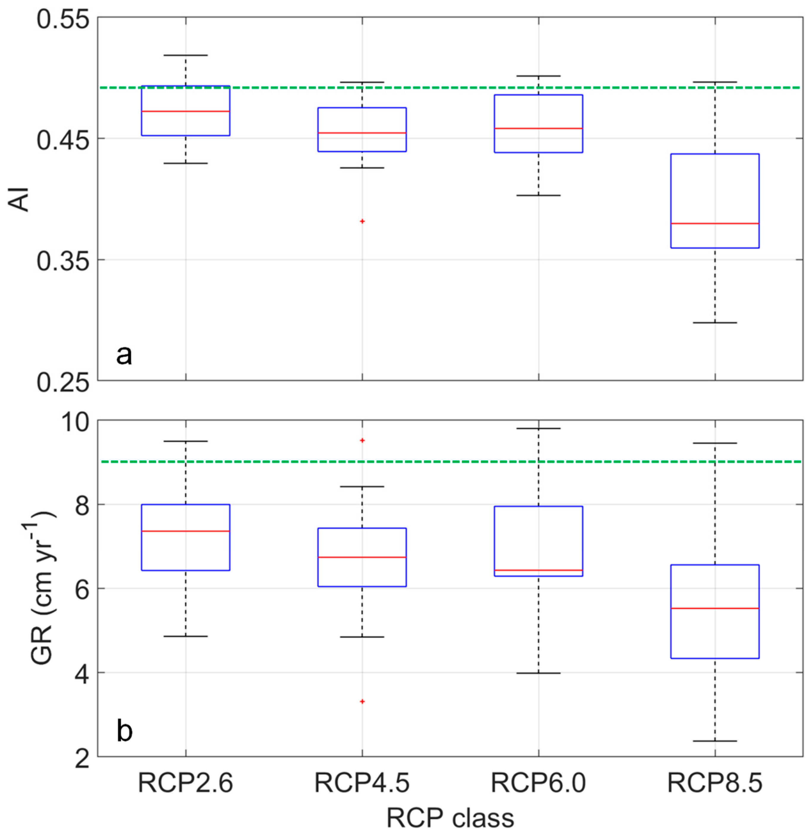
Due to the substantial differences in the rates of change between ET0 and P, the use of a synthetic climate measure such as the aridity index (AI) is effective to evaluate recharge rates between the historic and climate change projections. Figure 2a shows the box plots of the projected multi-decadal-average AI-values obtained from the 19 climate models for each emission scenario. The AI values resulting from the analysis were 0.47 ± 0.014, 0.45 ± 0.015, 0.46 ± 0.021, and 0.40 ± 0.029, for RCP2.6, RCP4.5, RCP6.0 and RCP8.5, respectively (see Equation (1)). These results suggest that the region is projected to become more arid (with decreasing AI-values) compared to the historical baseline (AI = 0.49) but still remaining in the same semi-arid class [59]. The greatest change in aridity is likely to occur only under the RCP8.5 climate projection scenario.
The ANOVA test at 5% significance level rejected the hypothesis that the mean AI values of the four groups were equal to each other given that F-value = 12.75 was larger than the critical F-value. However, if the AI-values of the RCP8.5 were removed, the ANOVA test would accept the hypothesis that the mean values of the RCP2.6, RCP4.5 and RCP6.0 group were significantly equal. This statistical analysis suggests that the change in aridity index under the climate change scenarios was only significant under the worst-case scenario.
The analysis also indicates that all climate scenarios caused a decline in GR rates compared to the historical baseline (9.02 cm yr−1). Projections of climate change induced a general decrease in the simulated potential GR, resulting in future period multi-decadal-averages of 7.15 ± 0.60 cm yr−1, 6.87 ± 0.71 cm yr−1, 6.95 ± 0.74 cm yr−1, and 5.51 ± 0.78 cm yr−1, for RCP2.6, RCP4.5, RCP6.0 and RCP8.5, respectively (see Equation (1)). The mean values represent decreases ranging from 21% in RCP2.6 to 39% in RCP8.5 in terms of percentage values (see box plots in Figure 2b). Nevertheless, box plots denote high uncertainty around the median value, with a coefficient of variation spanning from 18% to 30% for RCP2.6 and RCP8.5, respectively.
Lauffenburger et al. (2018) [58] reported that median annual recharge for the low (+1.0 °C, 478 ppm CO2) and high (+2.4 °C, 567 ppm CO2) global warming scenarios in western Nebraska rangeland are projected to decrease by about 9% and 94% relative to historical values, respectively.
The decrease in potential GR rates is due to a substantial increase in ET losses. This climatic setting also poses questions on probabilities related to plant survival, covered in Section 3.3.

3.2. Annual-Average Results of Historical and Projected AI, ETa, and GR

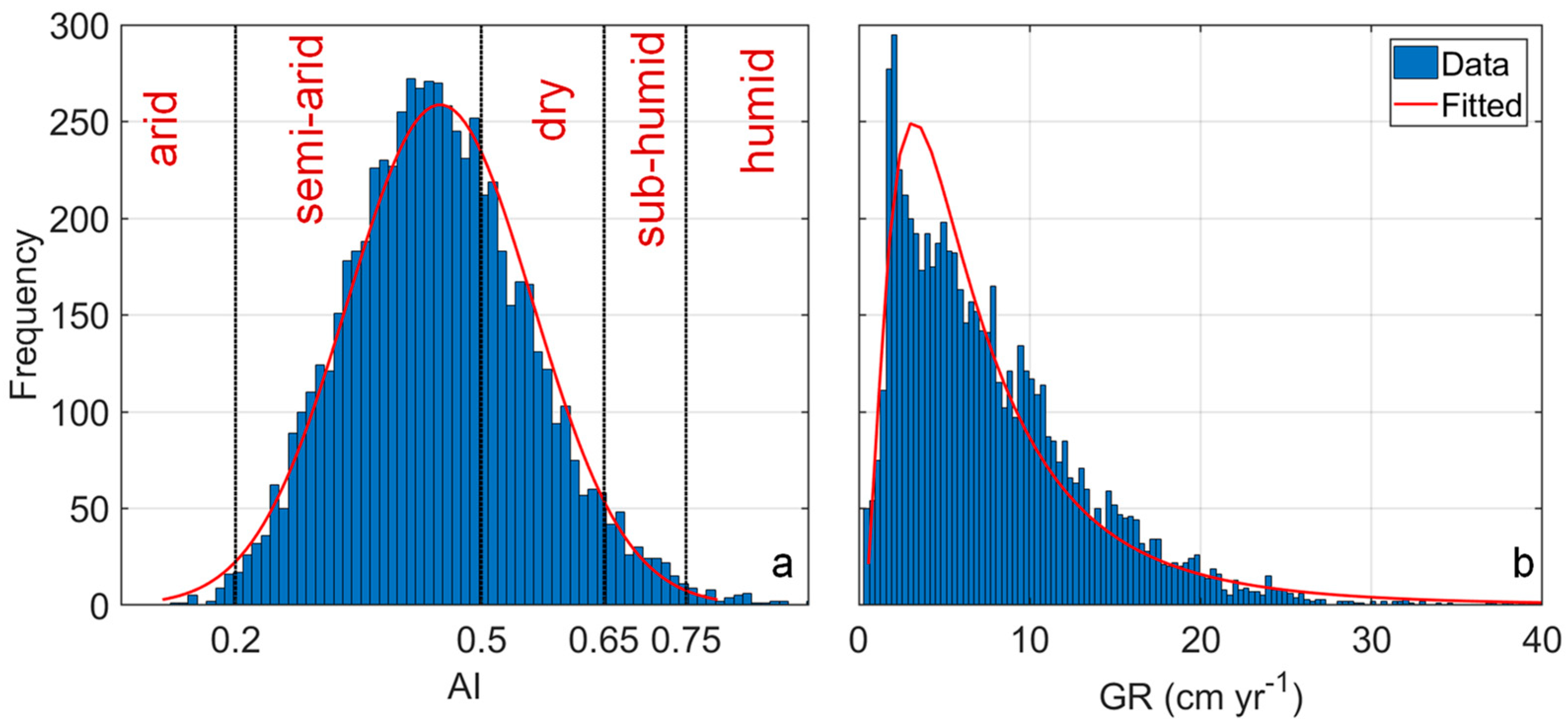
The model simulations comprise 50 years of historical and 100 years of 65 climate projections of climate forcings (P, ET0, ETp), aridity index (AI), and model output ETa and GR. The resulting annual-averages covering the projected 100-year simulation period are presented within a probabilistic framework shown in empirical histograms of AI values and corresponding GR (Figure 3). The normal and lognormal distributions (red lines) were fit on annual AI values and GR rates (blue histograms).
The probabilities for each climate class and corresponding median potential GR rates are reported in Table 2. Approximately 69% of the total aridity index values fall in the semi-arid climate class and are associated with the median potential GR rate (GR = 5.19 cm) that is significantly lower than the historic GR (9.02 cm yr−1, see Table A1). The probabilities of the climate shifting from semi-arid to dry (0.5 < AI ≤ 0.65) are approximately 26% and would produce a median potential GR of 9.64 cm yr−1, which is slightly greater (4.6%) than the historic value (9.02 cm yr−1). The combined probabilities attributed to extreme conditions such as arid, sub-humid, and humid climates were very low (~5%). The median-annual GR rates for the extreme climate conditions were far from the baseline rates.
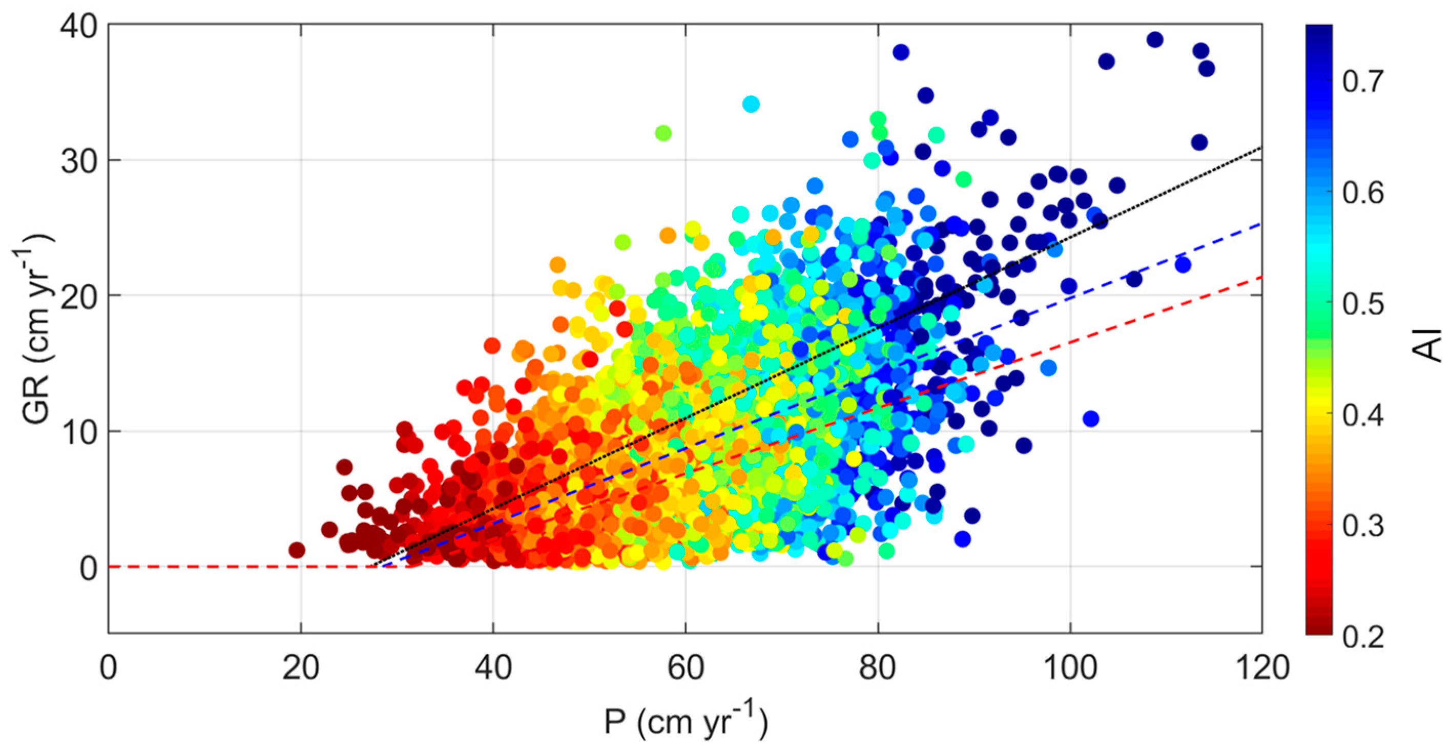
The coarse sandy soils in the Nebraska Sand Hills are not conducive to overland flow, thus the water balance of the soil profile is likely controlled by vertical hydrological processes, namely infiltration and ET. Moreover, precipitation is one of the main drivers of GR under semi-arid climate conditions [60]. The relationship between annual P and GR was quantified through regression lines and the corresponding coefficient of determination, namely the R-squared (R2), for evaluating its goodness of fit for both the historic and projected data group. The data are presented in Table 3 and visualized through a scatter plot in Figure 4, where the circles are colored according to the aridity index values.
Even though the regressions are clearly affected by heteroscedasticity (with higher spread around the regression line for higher AI-values), the results presented in Figure 4 and Table 3 represent a good opportunity to roughly estimate potential GR rates from projected P with annual temporal resolution. Given the R2-values listed in Table 3, P is able to explain about 30%–40% of GR temporal variability. It is apparent that all projected regression lines lie below the historic line (dotted black line), which means that GR rates will likely decrease, especially under the worst-case scenario (RCP8.5, dashed red line), as can be observed from the slopes of the regression lines reported in Table 3.

3.3. Selection of Three Representative Climate Projections for Assessing the Relation between Precipitation and Groundwater Recharge Rates at Sub-Annual Time Scale

Detailed results can be explored at sub-annual resolution. Nonetheless, it was not practical to analyze simulations pertaining to all climate projections. Therefore, for the purpose of encompassing the full spectrum of most probable future climate projections, three representative climate scenarios were selected following the procedure recommended by Rossman et al. (2018) [34]. The temporal dynamics of all cumulative GR rates, colored according to RCP, are shown in Figure 5a. The corresponding frequency distribution of final cumulative GR rates recorded for the year 2100 with sample mean, x ¯ , and standard deviation, s, is displayed in Figure 5b. The dry, mean, and wet GR projections selected based on this analysis were CSIRO (RCP8.5), GFDL_M1 (RCP2.6), and MPI_MR (RCP4.5), respectively (Table A1), based on the closest GR rates identified using the x ¯ s , x ¯ and x + s ¯ distribution criteria, respectively (Figure 5b).
The annual time series of ETa, P, ET0, and potential GR rates of the three representative scenarios are shown in Figure 6. While the projected multi-decadal-averages of P are 54.0 cm yr−1, 59.4 cm yr−1, 58.9 cm yr−1, in dry, mean, wet scenarios, respectively, the three ET0 time series are characterized by time-variant increasing rates as predicted in other semi-arid environments [61]. Thus, the corresponding AI time series (not shown) suggests that the climate might suffer from an increasing aridity even though the progressive shift does not change the projected climate class from the historical designation (semi-arid). The results of the analyses are consistent with Oglesby et al. (2015) [62] that suggested that while the form and seasonality of P will change in Nebraska, the annual amount of P may not vary substantially. Similarly, the report forecasts that Nebraska will likely experience temperature increases ranging from 4 to 5 °F under low emission scenario and 8 to 9 °F in the high emission scenario. Both emission scenarios would result in greater aridity index given that P would remain relatively stable.
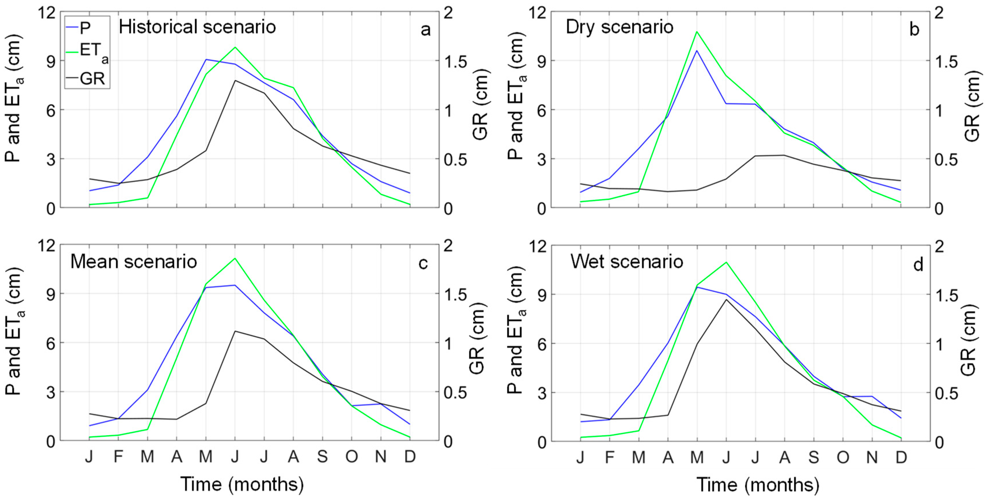
Annual-average groundwater recharge in the wet, mean, and dry projections are 8.40 cm yr−1, 6.74 cm yr−1, and 3.94 cm yr−1, representing −7%, −25% and −56% changes relative to the historical baseline (9.02 cm yr−1). Crosbie et al. (2013) [56] estimated a baseline historical recharge of 7.8 cm yr−1 for the Northern High Plains. The selected three future climate scenarios, namely dry, median, and wet correspond to 10%, 50%, and 90% exceedances for low (+1.0 °C, 478 ppm CO2), medium (+1.7 °C, 523 ppm CO2), and high (+2.4 °C, 567 ppm CO2) global warming scenarios. The study reported that GR was projected to be 5.93 cm yr−1 (−24%), 8.42 cm yr−1 (+8%), and 10.30 cm yr−1 (+32%) under the dry, median, wet scenarios, respectively. Rossman et al. (2018) [34] also found an increase in projected GR under both the median and wet projections at a rate of 0.27 cm yr−1 (+5%) and 2.21 cm yr−1 (+30%), and a decrease under the dry projection by 1.50 cm yr−1 (-40%) averaged over 2010–2099 relative to the baseline averaged over 2000–2009. However, it is worth noting the differences in the baseline historical recharge rates used between this analysis (9.02 cm yr−1) for NNF and Rossman et al. 2018 [34] (7.0 cm yr−1) for NSH. The difference in projected recharge rates may also have occurred due to simulation scales (spatial and temporal) and differences in the modeling approach. Spatial resolution differences can create discrepancies in the historical averages of climate forcings and the resulting parameters such as ETa and GR. While the focus of this study is on the NNF site, Crosbie et al. (2013) [56] and Rossman et al. (2018) [34] provide averaged values over Northern High Plains and the NSH, and make use of WAVES, a one-dimensional point-scale model that simulates the fluxes of mass and energy between the atmosphere, vegetation, and soil systems [63] and the variable infiltration capacity (VIC) macroscale hydrology model [64], respectively. Further, differences can also arise from the increased number of climate models used in this analysis, as opposed to the number of climate models used in Crosbie et al. (2013) [56] and Rossman et al. (2018) [34]. Despite these differences, GR rates are nearly equivalent to those reported in Crosbie et al. (2013) [56] when only looking at results derived from the same climate models. Discrepancies will continue to exist when comparing GR rates derived from averaging all climate projections over the entire NHP and NSH spatial extents. To describe and test the entirety of reasons for differences among previous studies was not an objective of this investigation, but it could be a focus for future research. In semi-arid regions, the impact of precipitation on GR is more important when analyzing the seasonal distribution rather than the annual sums [65]. The distribution of monthly sums of precipitation, actual ET, and potential GR highlights interesting aspects. Historic precipitation, actual ET and potential GR follow similar temporal trends with maxima in May (P = 9.07 cm), June (ETa = 9.82 cm), and June (GR = 1.30 cm). Minima occur in winter months likely related to negligible precipitation, low temperatures, and freezing conditions. The projected monthly distributions under the mean and wet scenarios roughly reproduce similar trends for P, while the dry scenario generates precipitation lower than the historic baseline during the summer seasons and higher than the historic baseline during the winter seasons. The dry climate projection indicates that summer months produce 17.4 cm yr−1 of P, which is a 25% reduction in summer month P compared to the historic value (23.1 cm yr−1). This significant water deficit is reflected in a 60% loss in GR rates in the summer, which is the major season for groundwater replenishment in this region. Spring is the next most important season for GR. However, GR was also substantially reduced in April and May months due to the projected excessive actual ET demand (+25%) in the dry scenario. Outside of the summer and spring months of the year, the values for the water balance components observed under the historic time period and the dry scenario projection were similar.
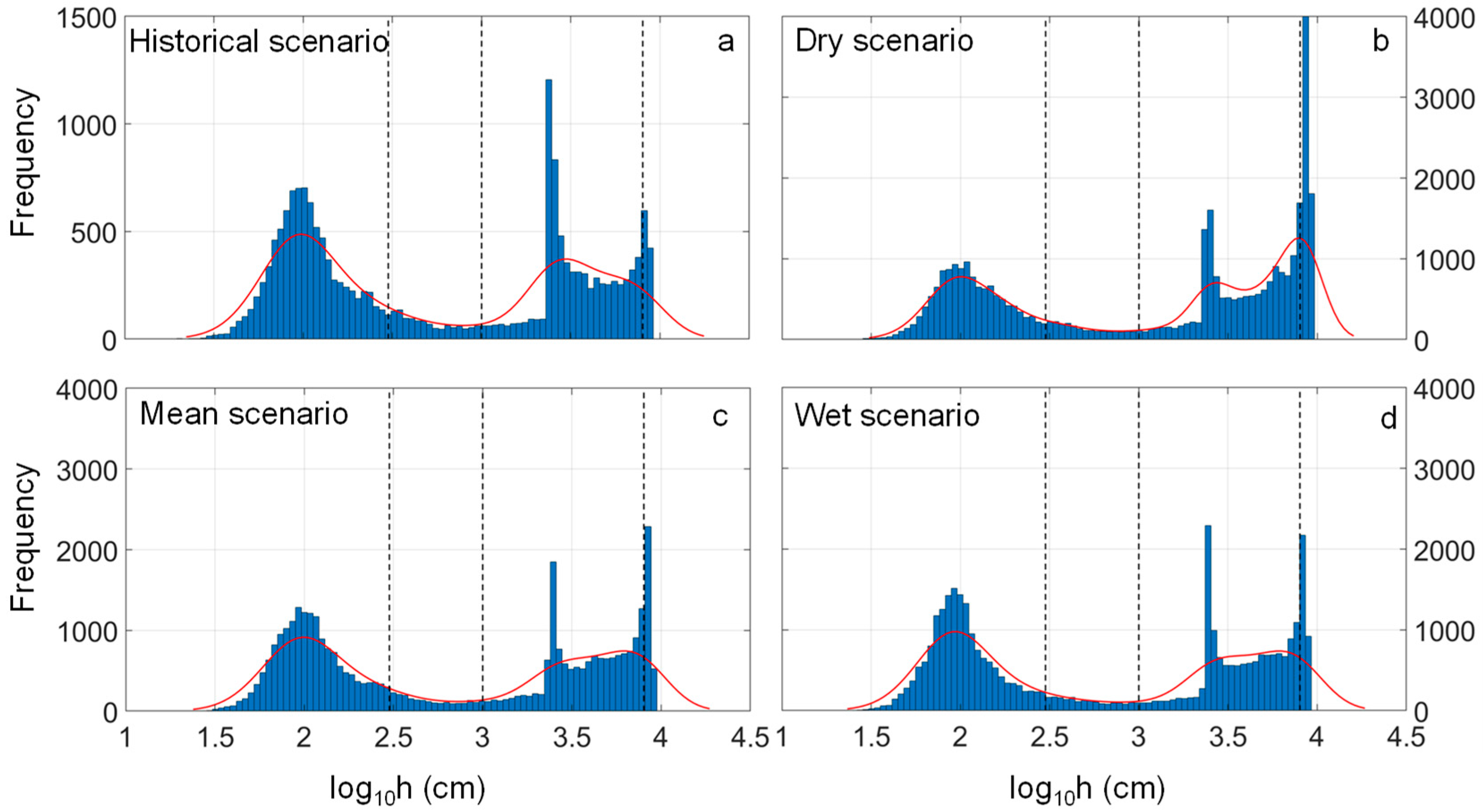
The water deficit detected by using monthly sums (Figure 7) poses the risk of threatening plant survival in this site. In this study, we applied time-invariant parameters for root water uptake as we assumed no change in grassland cover in HYDRUS-1D [17]. Prolonged root water stress is known to cause plant wilting and subsequent withering. Increasing chances of root water stress induced by a change in climate will have consequences to the native grassland ecology of the Nebraska Sand Hills. In this study, daily values of root water stress were explored in the historical data and the mean, wet, and dry scenario projections. Frequency distribution of decimal logarithmic values (18,262 daily values) of pressure head at root depth was used to explore the impact of climate change on grassland root water stress. The results were fitted by using a nonparametric kernel probability smoothing distribution.
The root water stress analysis was performed within a probabilistic framework, where the probabilities associated with no-stress, stress, and wilting point were considered (Table 4). The analysis indicates that the historic conditions resulted in equivalent percentages of root water stress and no stress conditions (about 49% and 47%, respectively) as well as low probabilities (4.3%) to reach wilting points. While the root water stress probabilities under the mean and wet climate projections were equivalent to the historic condition, the wilting point probabilities under the projections nearly double from 4.3% to 8.5% (Table 4). In contrast, the dry scenario analysis indicates that while the stress probability remains equivalent, the no stress probability is considerably reduced from 48.8% to 35.1%. Of particular interest is also a significant increase in the probability of wilting point (Figure 8). The wilting point probability under the dry climate scenario increased about four times compared to the historic condition. This analysis indicates that the conditions that would be induced by the dry scenario will increase the risk for grass to die and increase the chance of desertification of this region substantially.

4. Conclusions

The study examined the relationship between historic (1950–2000) and projected future (2000–2100) climate forcings and the GR rates in a site-specific study in the Nebraska National Forest of the Nebraska Sand Hills region. Toward this objective, we considered 65 projections of GR that included four greenhouse gas emissions scenarios. These climate inputs were used in the local-scale numerical model of soil-atmosphere-vegetation dynamics based on HYDRUS-1D. The results have been averaged over decadal, annual, and sub-annual time scales within a probabilistic framework accounting for uncertainty in climate projections. Dry, mean, and wet GR recharge scenarios were defined from the statistical parameters of cumulative GR from daily model runs. The historic climate in the NSH is classified as semi-arid with annual-average potential GR rate of 9.02 cm yr−1. Projections of decadal precipitation appear to remain quasi-steady with negligible (1%) increase while increasing forecasts of ET0 range from 8.6% to 31.4%. These main factors are shown to cause a decrease in decadal GR rates ranging from 21% to 39% in extreme cases. It is also worth noting that the Hargreaves approach to estimate ET0 can inject uncertainty in recharge estimation. In this analysis, the results indicate that GR will likely be overestimated if ET0 is estimated using the Hargreaves equation. In contrast, GR is likely to be even lower if ET0 is estimated by using the Penman-Monteith equation.
The results highlight the need to consider adaptation and mitigation measures to respond to projected decreases in GR, which can exacerbate groundwater depletion in the High Plains Aquifer. The outcomes also underscore the need for exploring measures to combat the projected potential increases in wilting probability (~8.3% to 18.5% compared to 4.3% historical baseline), to protect the native grassland ecosystem, and to prevent desertification processes.

Author Contributions

For research articles with several authors, a short paragraph specifying their individual contributions must be provided. The following statements should be used “conceptualization, Z.A., P.N., N.R., T.W. and V.Z.; methodology, Z.A. and P.N.; software, P.N. and Z.A.; validation, P.N., Z.A., N.R. and T.W.; formal analysis, Z.A., P.N., N.R., T.W. and V.Z.; investigation, Z.A. and P.N.; resources, V.Z.; data curation, P.N.; writing—original draft preparation, P.N. and Z.A.; writing—review and editing, Z.A., P.N., N.R., T.W. and V.Z.; visualization, X.X.; supervision, V.Z. and P.N.; project administration, V.Z.; funding acquisition, V.Z.

Funding

The authors acknowledge the financial support provided by the NSF IGERT program (DGE-0903469), the Nebraska Geological Society’s Yatkola-Edwards scholarship and the American Association of Petroleum Geologists.

Conflicts of Interest

The authors declare no conflict of interest.

Appendix A

Table A1. Multi-decadal-average values of P, ET0, AI, ETp, ETa, and GR for historic data and different RCP classes.
Data SetsModelPET0AIETpETaGR
cm yr−1cm yr−1-cm yr−1cm yr−1cm yr−1
Historic data 1950–2000NA55.7114.10.4978.545.89.02
RCP 2.6
2000–2100
BCC_CSM56.9124.00.4685.349.28.0
CANESM58.0127.90.4587.648.56.9
CCSM59.8123.10.4984.549.28.2
CESM_BGCn.a.n.a.n.a.n.a.n.a.n.a.
CNRM_CMn.a.n.a.n.a.n.a.n.a.n.a.
CSIRO56.6125.30.4586.646.07.2
GFDL_CM66.3127.40.5287.855.47.5
GFDL_G155.7122.20.4684.347.85.8
GFDL_M159.4119.60.5082.048.06.7
INMCMn.a.n.a.n.a.n.a.n.a.n.a.
IPSL_CM57.9123.30.4786.449.15.9
IPSL_MR56.2124.60.4585.346.97.0
MIROC_ESM59.3129.00.4687.346.89.5
MIRCO_ESM60.6128.40.4788.949.57.4
MICROC53.9125.60.4385.547.34.9
MPI_LR56.4120.70.4783.048.66.3
MPI_MR61.9120.40.5182.850.69.2
MRI_GCM58.6117.10.5080.650.25.9
NORESM62.7122.20.5184.251.68.0
RCP 4.5
2000–2100
BCC_CSM56.2126.60.4487.747.27.4
CANESM58.3129.80.4589.348.47.2
CCSM57.5126.80.4588.246.96.2
CESM_BGC59.6125.10.4885.948.17.7
CNRM_CM58.2124.30.4785.547.48.5
CSIRO55.7128.60.4388.046.56.3
GFDL_CMn.a.n.a.n.a.n.a.n.a.n.a.
GFDL_G159.5123.70.4885.349.86.0
GFDL_M160.7120.90.5082.750.76.0
INMCM54.5121.70.4583.844.87.5
IPSL_CM53.7127.60.4289.447.34.8
IPSL_MR54.1128.30.4287.745.76.8
MIROC_ESM60.3131.60.4689.749.09.5
MIRCO_ESM60.8133.00.4690.249.57.4
MICROC49.4132.80.3789.744.13.3
MPI_LR56.5124.20.4585.647.56.7
MPI_MR58.9124.80.4785.848.98.4
MRI_GCM58.7119.80.4982.449.85.6
NORESM59.1127.10.4687.550.88.4
RCP 6.0
2000–2100
BCC_CSM61.7126.10.4987.049.19.8
CANESMn.a.n.a.n.a.n.a.n.a.n.a.
CCSM56.2126.60.4487.247.56.3
CESM_BGCn.a.n.a.n.a.n.a.n.a.n.a.
CNRM_CMn.a.n.a.n.a.n.a.n.a.n.a.
CSIROn.a.n.a.n.a.n.a.n.a.n.a.
GFDL_CM65.3128.50.5188.655.28.2
GFDL_G159.0124.20.4785.250.96.4
GFDL_M159.3121.90.4983.749.37.2
INMCMn.a.n.a.n.a.n.a.n.a.n.a.
IPSL_CM55.7126.50.4488.246.66.3
IPSL_MR52.5129.10.4188.243.66.4
MIROC_ESM60.1130.80.4688.848.67.7
MIRCO_ESM59.6131.60.4589.348.58.9
MICROC52.4128.40.4188.145.94.0
MPI_LRn.a.n.a.n.a.n.a.n.a.n.a.
MPI_MRn.a.n.a.n.a.n.a.n.a.n.a.
MRI_GCM58.2118.50.4981.850.65.8
NORESM57.4126.10.4686.548.46.4
RCP 8.5
2000–2100
BCC_CSM60.8163.20.3789.748.59.5
CANESM62.4133.50.47112.652.66.8
CCSM61.0165.10.37110.151.55.5
CESM_BGC60.7128.00.47107.652.15.6
CNRM_CM56.7128.70.44108.449.25.2
CSIRO54.0131.80.41111.748.03.9
GFDL_CM67.8131.40.52110.858.46.6
GFDL_G159.0161.80.36109.252.24.8
GFDL_M160.2158.10.38107.151.86.4
INMCM53.2125.60.42108.346.55.1
IPSL_CM54.7164.90.33113.347.84.0
IPSL_MR49.8166.90.30112.744.33.4
MIROC_ESM60.3170.50.35112.850.67.8
MIRCO_ESM61.5170.40.36113.552.46.1
MICROC51.8167.80.31111.747.32.4
MPI_LR54.8130.90.42110.448.64.2
MPI_MR61.2127.70.48108.150.86.6
MRI_GCM61.0153.70.40104.052.95.6
NORESM57.7165.90.35111.550.25.3

References

  1. Eckhardt, K.; Ulbrich, U. Potential impacts of climate change on groundwater recharge and streamflow in a central European low mountain range. J. Hydrol. 2003, 284, 244–252. [Google Scholar] [CrossRef]
  2. Ng, G.-H.C.; McLaughlin, D.; Entekhabi, D.; Scanlon, B.R. Probabilistic analysis of the effects of climate change on groundwater recharge. Water Resour. Res. 2010, 46, 1–18. [Google Scholar] [CrossRef]
  3. Kim, J.H.; Jackson, R.B. A Global Analysis of Groundwater Recharge for Vegetation, Climate, and Soils. Vadose Zone J. 2012, 11. [Google Scholar] [CrossRef] [Green Version]
  4. Nasta, P.; Gates, J.B.; Wada, Y. Impact of climate indicators on continental-scale potential groundwater recharge in Africa. Hydrol. Process. 2016, 30, 3420–3433. [Google Scholar] [CrossRef] [PubMed]
  5. Terrell, B.L.; Johnson, P.N.; Segarra, E. Ogallala aquifer depletion: Economic impact on the Texas high plains. Water Policy 2002, 4, 33–46. [Google Scholar] [CrossRef]
  6. Scanlon, B.R.; Keese, K.E.; Flint, A.L.; Flint, L.E.; Gaye, C.B.; Edmunds, W.M.; Simmers, I. Global synthesis of groundwater recharge in semiarid and arid regions. Hydrol. Process. 2006, 20, 3335–3370. [Google Scholar] [CrossRef]
  7. Cheng, L.; Hoerling, M.; Aghakouchak, A.; Livneh, B.; Quan, X.W.; Eischeid, J. How has human-induced climate change affected California drought risk? J. Clim. 2016, 29, 111–120. [Google Scholar] [CrossRef]
  8. Carson, M.; Köhl, A.; Stammer, D.; Slangen, A.A.B.; Katsman, C.A.; van de Wal, R.S.W.; Church, J.; White, N. Coastal sea level changes, observed and projected during the 20th and 21st century. Clim. Chang. 2016, 134, 269–281. [Google Scholar] [CrossRef]
  9. Turco, M.; Llasat, M.C.; von Hardenberg, J.; Provenzale, A. Climate change impacts on wildfires in a Mediterranean environment. Clim. Chang. 2014, 125, 369–380. [Google Scholar] [CrossRef]
  10. Mori, N.; Yasuda, T.; Mase, H.; Tom, T.; Oku, Y. Projection of Extreme Wave Climate Change under Global Warming. Hydrol. Res. Lett. 2010, 4, 15–19. [Google Scholar] [CrossRef]
  11. Arnell, N.W.; Gosling, S.N. The impacts of climate change on river flood risk at the global scale. Clim. Chang. 2016, 134, 387–401. [Google Scholar] [CrossRef]
  12. Bellard, C.; Bertelsmeier, C.; Leadley, P.; Thuiller, W.; Courchamp, F. Impacts of climate change on the future of biodiversity. Ecol. Lett. 2012, 15, 365–377. [Google Scholar] [CrossRef] [PubMed] [Green Version]
  13. Gunkel, A.; Shadeed, S.; Hartmann, A.; Wagener, T.; Lange, J. Model signatures and aridity indices enhance the accuracy of water balance estimations in a data-scarce Eastern Mediterranean catchment. J. Hydrol. Reg. Stud. 2015, 4, 487–501. [Google Scholar] [CrossRef] [Green Version]
  14. Milly, P.C.D.; Dunne, K.A. Potential evapotranspiration and continental drying. Nat. Clim. Chang. 2016, 6, 946. [Google Scholar] [CrossRef]
  15. Trenberth, K.E. Changes in precipitation with climate change. Clim. Res. 2011, 47, 123–138. [Google Scholar] [CrossRef] [Green Version]
  16. Graham, L.P.; Andreáasson, J.; Carlsson, B. Assessing climate change impacts on hydrology from an ensemble of regional climate models, model scales and linking methods—A case study on the Lule River basin. Clim. Chang. 2007, 81, 293–307. [Google Scholar] [CrossRef]
  17. Kling, H.; Fuchs, M.; Paulin, M. Runoff conditions in the upper Danube basin under an ensemble of climate change scenarios. J. Hydrol. 2012, 424–425, 264–277. [Google Scholar] [CrossRef]
  18. Huang, J.; Zhang, Z.; Feng, Y.; Hong, H. Hydrologic response to climate change and human activities in a subtropical coastal watershed of southeast China. Reg. Environ. Chang. 2013, 13, 1195–1210. [Google Scholar] [CrossRef]
  19. López-Moreno, J.I.; Zabalza, J.; Vicente-Serrano, S.M.; Revuelto, J.; Gilaberte, M.; Azorin-Molina, C.; Morán-Tejeda, E.; García-Ruiz, J.M.; Tague, C. Impact of climate and land use change on water availability and reservoir management: Scenarios in the Upper Arago’n River, Spanish Pyrenees. Sci. Total Environ. 2014, 493, 1222–1231. [Google Scholar] [CrossRef]
  20. Le Roux, P.C.; Aalto, J.; Luoto, M. Soil moisture’s underestimated role in climate change impact modelling in low-energy systems. Glob. Chang. Biol. 2013, 19, 2965–2975. [Google Scholar] [CrossRef]
  21. Goderniaux, P.; Brouyère, S.; Fowler, H.J.; Blenkinsop, S.; Therrien, R.; Orban, P.; Dassargues, A. Large scale surface-subsurface hydrological model to assess climate change impacts on groundwater reserves. J. Hydrol. 2009, 373, 122–138. [Google Scholar] [CrossRef]
  22. Herrmann, F.; Baghdadi, N.; Blaschek, M.; Deidda, R.; Duttmann, R.; La Jeunesse, I.; Sellami, H.; Vereecken, H.; Wendland, F. Simulation of future groundwater recharge using a climate model ensemble and SAR-image based soil parameter distributions—A case study in an intensively-used Mediterranean catchment. Sci. Total Environ. 2016, 543, 889–905. [Google Scholar] [CrossRef]
  23. Meixner, T.; Manning, A.H.; Stonestrom, D.A.; Allen, D.M.; Ajami, H.; Blasch, K.W.; Brookfield, A.E.; Castro, C.L.; Clark, J.F.; Gochis, D.J.; et al. Implications of projected climate change for groundwater recharge in the western United States. J. Hydrol. 2016, 534, 124–138. [Google Scholar] [CrossRef] [Green Version]
  24. Taylor, R.G.; Scanlon, B.; Döll, P.; Rodell, M.; Van Beek, R.; Wada, Y.; Longuevergne, L.; Leblanc, M.; Famiglietti, J.S.; Edmunds, M.; et al. Ground water and climate change. Nat. Clim. Chang. 2013, 3, 322. [Google Scholar] [CrossRef]
  25. Kitabata, H.; Nishizawa, K.; Yoshida, Y.; Maruyama, K. Permafrost Thawing in Circum-Arctic and Highlands under Climatic Change Scenario Projected by Community Climate System Model (CCSM3). SOLA 2006, 2, 53–56. [Google Scholar] [CrossRef] [Green Version]
  26. Nyenje, P.M.; Batelaan, O. Estimating the effects of climate change on groundwater recharge and baseflow in the upper Ssezibwa catchment, Uganda. Hydrol. Sci. J. 2009, 54, 713–726. [Google Scholar] [CrossRef] [Green Version]
  27. Crosbie, R.S.; McCallum, J.L.; Walker, G.R.; Chiew, F.H.S. Modelling climate-change impacts on groundwater recharge in the Murray-Darling Basin, Australia. Hydrogeol. J. 2010, 18, 1639–1656. [Google Scholar] [CrossRef]
  28. Goodarzi, M.; Abedi-Koupai, J.; Heidarpour, M.; Safavi, H.R. Evaluation of the Effects of Climate Change on Groundwater Recharge Using a Hybrid Method. Water Resour. Manag. 2016, 30, 133–148. [Google Scholar] [CrossRef]
  29. Bouraoui, F.; Vachaud, G.; Li, L.Z.X.; Le Treut, H.; Chen, T. Evaluation of the impact of climate changes on water storage and groundwater recharge at the watershed scale. Clim. Dyn. 1999, 15, 153–161. [Google Scholar] [CrossRef]
  30. Green, T.R.; Taniguchi, M.; Kooi, H.; Gurdak, J.J.; Allen, D.M.; Hiscock, K.M.; Treidel, H.; Aureli, A. Beneath the surface of global change: Impacts of climate change on groundwater. J. Hydrol. 2011, 405, 532–560. [Google Scholar] [CrossRef]
  31. Rossman, N.R.; Zlotnik, V.A.; Rowe, C.M.; Szilagyi, J. Vadose zone lag time and potential 21st century climate change effects on spatially distributed groundwater recharge in the semi-arid Nebraska Sand Hills. J. Hydrol. 2014, 519, 656–669. [Google Scholar] [CrossRef] [Green Version]
  32. Adane, Z.; Nasta, P.; Gates, J.B. Links between soil hydrophobicity and groundwater recharge under plantations in a sandy grassland setting, Nebraska Sand Hills, USA. For. Sci. 2017, 63, 388–401. [Google Scholar] [CrossRef]
  33. Adane, Z.A.; Nasta, P.; Zlotnik, V.; Wedin, D. Impact of grassland conversion to forest on groundwater recharge in the Nebraska Sand Hills. J. Hydrol. Reg. Stud. 2018, 15, 171–183. [Google Scholar] [CrossRef]
  34. Rossman, N.R.; Zlotnik, V.A.; Rowe, C.M. Using cumulative potential recharge for selection of GCM projections to force regional groundwater models: A Nebraska Sand Hills example. J. Hydrol. 2018, 561, 1105–1114. [Google Scholar] [CrossRef]
  35. Miao, X.; Mason, J.A.; Johnson, W.C.; Wang, H. High-resolution proxy record of Holocene climate from a loess section in Southwestern Nebraska, USA. Palaeogeogr. Palaeoclimatol. Palaeoecol. 2007, 245, 368–381. [Google Scholar] [CrossRef]
  36. Wang, T.; Wedin, D.; Zlotnik, V.A. Field evidence of a negative correlation between saturated hydraulic conductivity and soil carbon in a sandy soil. Water Resour. Res. 2009. [Google Scholar] [CrossRef]
  37. Scanlon, B.R.; Faunt, C.C.; Longuevergne, L.; Reedy, R.C.; Alley, W.M.; McGuire, V.L.; McMahon, P.B. Groundwater depletion and sustainability of irrigation in the US High Plains and Central Valley. Proc. Natl. Acad. Sci. USA 2012, 109, 9320–9325. [Google Scholar] [CrossRef] [Green Version]
  38. Allen, R.G. FAO Irrigation and Drainage Paper Crop by. Irrig. Drain. 1998, 300, 300. [Google Scholar]
  39. Adane, Z.A.; Gates, J.B. Determining the impacts of experimental forest plantation on groundwater recharge in the Nebraska Sand Hills (USA) using chloride and sulfate. Hydrogeol. J. 2015, 23, 81–94. [Google Scholar] [CrossRef]
  40. Hargreaves, G.H.; Allen, R.G. History and Evaluation of Hargreaves Evapotranspiration Equation. J. Irrig. Drain. Eng. 2003, 129, 53–63. [Google Scholar] [CrossRef]
  41. Pelosi, A.; Medina, H.; Villani, P.; D’Urso, G.; Chirico, G.B. Probabilistic forecasting of reference evapotranspiration with a limited area ensemble prediction system. Agric. Water Manag. 2016, 178, 106–118. [Google Scholar] [CrossRef]
  42. Droogers, P.; Allen, R.G. Estimating reference evapotranspiration under inaccurate data conditions. Irrig. Drain. Syst. 2002, 16, 33–45. [Google Scholar] [CrossRef]
  43. Archibald, J.A.; Walter, M.T. Do energy-based PET models require more input data than temperature-based models?—An evaluation at four humid fluxnet sites. J. Am. Water Resour. Assoc. 2014, 50, 497–508. [Google Scholar] [CrossRef]
  44. Huo, Z.; Dai, X.; Feng, S.; Kang, S.; Huang, G. Effect of climate change on reference evapotranspiration and aridity index in arid region of China. J. Hydrol. 2013, 492, 24–34. [Google Scholar] [CrossRef]
  45. Liu, X.; Zhang, D.; Luo, Y.; Liu, C. Spatial and temporal changes in aridity index in northwest China: 1960 to 2010. Theor. Appl. Climatol. 2013, 112, 307–316. [Google Scholar] [CrossRef]
  46. Nastos, P.T.; Politi, N.; Kapsomenakis, J. Spatial and temporal variability of the Aridity Index in Greece. Atmos. Res. 2013, 119, 140–152. [Google Scholar] [CrossRef]
  47. Zhang, K.X.; Pan, S.M.; Zhang, W.; Xu, Y.H.; Cao, L.G.; Hao, Y.P.; Wang, Y. Influence of climate change on reference evapotranspiration and aridity index and their temporal-spatial variations in the Yellow River Basin, China, from 1961 to 2012. Quat. Int. 2015, 380, 75–82. [Google Scholar] [CrossRef]
  48. Arora, V.K. The use of the aridity index to assess climate change effect on annual runoff. J. Hydrol. 2002, 265, 164–177. [Google Scholar] [CrossRef]
  49. Nkomozepi, T.; Chung, S.O. The effects of climate change on the water resources of the Geumho River Basin, Republic of Korea. J. Hydro-Environ. Res. 2014, 8, 358–366. [Google Scholar] [CrossRef]
  50. Gudmundsson, L.; Greve, P.; Seneviratne, S.I. The sensitivity of water availability to changes in the aridity index and other factors—A probabilistic analysis in the Budyko space. Geophys. Res. Lett. 2016, 43, 6985–6994. [Google Scholar] [CrossRef]
  51. Šimůnek, J.; van Genuchten, M.T.; Šejna, M. Recent developments and applications of the HYDRUS computer software packages. Vadose Zone J. 2016, 15, 25. [Google Scholar] [CrossRef]
  52. Nasta, P.; Gates, J.B. Plot-scale modeling of soil water dynamics and impacts of drought conditions beneath rainfed maize in Eastern Nebraska. Agric. Water Manag. 2013, 128, 120–130. [Google Scholar] [CrossRef]
  53. Van Genuchten, M.T. A Closed-form Equation for Predicting the Hydraulic Conductivity of Unsaturated Soils1. Soil Sci. Soc. Am. J. 1980, 44, 892. [Google Scholar] [CrossRef]
  54. Spinoni, J.; Vogt, J.; Naumann, G.; Carrao, H.; Barbosa, P. Towards identifying areas at climatological risk of desertification using the Köppen-Geiger classification and FAO aridity index. Int. J. Climatol. 2015, 35, 2210–2222. [Google Scholar] [CrossRef]
  55. Billesbach, D.P.; Arkebauer, T.J. First long-term, direct measurements of evapotranspiration and surface water balance in the Nebraska SandHills. Agric. For. Meteorol. 2012, 156, 104–110. [Google Scholar] [CrossRef] [Green Version]
  56. Crosbie, R.S.; Scanlon, B.R.; Mpelasoka, F.S.; Reedy, R.C.; Gates, J.B.; Zhang, L. Potential climate change effects on groundwater recharge in the High Plains Aquifer, USA. Water Resour. Res. 2013, 49, 3936–3951. [Google Scholar] [CrossRef] [Green Version]
  57. Szilagyi, J.; Zlotnik, V.A.; Gates, J.B.; Jozsa, J. Mapping mean annual groundwater recharge in the Nebraska Sand Hills, USA. Hydrogeol. J. 2011, 19, 1503–1513. [Google Scholar] [CrossRef]
  58. Lauffenburger, Z.H.; Gurdak, J.J.; Hobza, C.; Woodward, D.; Wolf, C. Irrigated agriculture and future climate change effects on groundwater recharge, northern High Plains aquifer, USA. Agric. Water Manag. 2018, 204, 69–80. [Google Scholar] [CrossRef]
  59. Greve, P.; Seneviratne, S.I. Assessment of future changes in water availability and aridity. Geophys. Res. Lett. 2015, 42, 5493–5499. [Google Scholar] [CrossRef] [Green Version]
  60. Thomas, B.F.; Behrangi, A.; Famiglietti, J.S. Precipitation intensity effects on groundwater recharge in the southwestern United States. Water 2016, 8, 90. [Google Scholar] [CrossRef]
  61. Tabari, H.; Aghajanloo, M.B. Temporal pattern of aridity index in Iran with considering precipitation and evapotranspiration trends. Int. J. Climatol. 2013, 33, 396–409. [Google Scholar] [CrossRef]
  62. Oglesby, R.; Bathke, D.; Wilhite, D.; Rowe, C. Understanding and assessing projected future climate change for Nebraska and the great plains. Gt. Plains Res. 2015, 25, 97–107. [Google Scholar] [CrossRef]
  63. Dawes, W.; Zhang, L.; Dyce, P. WAVES V3.5 user manual. Available online: https://research.csiro.au/software/wp-content/uploads/sites/6/2016/07/preface.pdf (accessed on 4 September 2018).
  64. Liang, X.; Lettenmaier, D.P.; Wood, E.F.; Burges, S.J. A simple hydrologically based model of land surface water and energy fluxes for general circulation models. J. Geophys. Res. 2004, 99, 14415–14428. [Google Scholar] [CrossRef]
  65. Nasta, P.; Adane, Z.; Lock, N.; Houston, A.; Gates, J.B. Links between episodic groundwater recharge rates and rainfall events classified according to stratiform-convective storm scoring: A plot-scale study in eastern Nebraska. Agric. For. Meteorol. 2018, 259, 154–161. [Google Scholar] [CrossRef]
Figure 1. Location of the study area—Nebraska National Forest, (NNF), Nebraska Sand Hills (NSH), High Plains Aquifer (HPA), experimental grassland plot site (G), and Middle Loup and Dismal rivers.
Water 11 00950 g001
Figure 2. Box plots of annual-averages (a) aridity index (AI) values and (b) groundwater recharge (GR) values classified according to the four RCPs. The horizontal dashed green line depicts the historic value.
Water 11 00950 g002
Figure 3. Frequency distribution (blue histograms) and fitted distribution (red lines) for (a) normally distributed aridity index, classified into arid, semi-arid, dry, sub-humid, and humid classes; and (b) lognormally distributed potential groundwater recharge rates.
Water 11 00950 g003
Figure 4. Scatter plot representing the relationship between annual-average P and GR with circle colors determined by the aridity index. The regression lines are showed for historic data (dotted black line), RCP2.6 (dashed blue line) and RCP8.5 (dashed red line).
Water 11 00950 g004
Figure 5. (a) Dynamics of cumulative GR rate projections from 2000 to 2100 under the four emission scenarios (blue, green, magenta and red lines represent RCP2.6, RCP4.5, RCP6.0 and RCP8.5, respectively); (b) frequency distribution (blue histograms) of the final cumulative GR-values with corresponding fitted normal distribution (red line) with mean ( x ¯ ) and standard deviation (s) that are used to select three representative climate projections (dry, mean and wet given by x ¯ s , x ¯ , and x ¯ + s , respectively)
Water 11 00950 g005
Figure 6. Historic and projected trends (dry, mean and wet projections) in annual averages of precipitation (P), reference evapotranspiration (ET0), and potential groundwater recharge (GR) rates.
Water 11 00950 g006
Figure 7. Monthly averages of precipitation (blue line), actual evapotranspiration (green), and potential groundwater recharge (GR; black line) under (a) historical records, (b) dry, (c) mean and (d) wet climate projections. P and ETa are referred to in the primary y-axis while GR is referred to in the secondary y-axis.
Water 11 00950 g007
Figure 8. Frequency distribution (blue histograms) and fitted nonparametric kernel probabilistic distribution (red line) of matric pressure head (in log10) under (a) historical records, (b) dry, (c) mean and (d) wet climate projections. Vertical dashed lines indicate the Feddes’ parameters controlling root water uptake.
Water 11 00950 g008
Table 1. Selected 19 global climate models used in this study and corresponding institutions.
AcronymInstitution
1BCC_CSMBeijing Climate Center (China)
2CANESMCanadian Centre for Climate Modelling and Analysis (Canada)
3CCSMUniversity Corporation for Atmospheric Research (UCAR) (USA)
4CESM_BGCNCAR Earth System Laboratory (USA)
5CNRM_CMNational Centre for Meteorological Research
6CSIROCommonwealth Scientific and Industrial Research Organization (Australia)
7GFDL_CMGeophysical Fluid Dynamics Laboratory (USA)
8GFDL_G1Geophysical Fluid Dynamics Laboratory (USA)
9GFDL_M1Geophysical Fluid Dynamics Laboratory (USA)
10INMCMInstitute of Numerical Mathematics (Russia)
11IPSL_CMInstitute Pierre-Simon Laplace (France)
12IPSL_MRInstitute Pierre-Simon Laplace (France)
13MIROC_ESMJapan Agency for Marine-Earth Science and Technology (Japan)
14MIRCO_ESMJapan Agency for Marine-Earth Science and Technology (Japan)
15MICROCJapan Agency for Marine-Earth Science and Technology (Japan)
16MPI_LRMax Planck Institute (Germany)
17MPI_MRMax Planck Institute (Germany)
18MRI_GCMMeteorological Research Institute (Japan)
19NORESMNorwegian Climate Center (Norway)
Table 2. Probabilities of annual AI-values and associated median annual potential groundwater recharge (GR) rates.
ValueClassProbabilityMedian GR
%cm yr−1
AI ≤ 0.2Arid0.561.87
0.2 < AI ≤ 0.5Semi-arid68.585.19
0.5 < AI ≤ 0.65Dry26.249.64
0.65 < AI ≤ 0.75Sub-humid3.7614.19
A > 0.75Humid0.8621.93
Table 3. Regression lines and corresponding goodness of fit (R2) for historical data and the four climate projections (RCP2.6, RCP4.5, RCP6.0, and RCP8.5).
ScenarioRegression LineR2
HistoricGR = 0.335P − 9.060.407
RCP2.6GR = 0.2767P − 7.870.351
RCP4.5GR = 0.2829P − 8.370.371
RCP6.0GR = 0.2794P − 8.330.351
RCP8.5GR = 0.2419P − 7.640.349
Table 4. Statistical probabilities (%) of no root water stress, root water stress, and wilting point conditions under historic records and dry, mean, wet climate projections.
ScenarioNo StressStressWilting Point
%%%
Historic48.846.94.3
Dry35.146.418.5
Mean46.145.48.5
Wet46.944.88.3