Article

The Use of Large-Scale Climate Indices in Monthly Reservoir Inflow Forecasting and Its Application on Time Series and Artificial Intelligence Models

1
School of Civil and Environmental Engineering, Yonsei University, Seoul 03722, Korea
2
National Institute of Meteorological Science, Seogwipo 63568, Korea
*
Author to whom correspondence should be addressed.
Water 2019, 11(2), 374; https://doi.org/10.3390/w11020374
Submission received: 30 October 2018 / Revised: 2 January 2019 / Accepted: 13 February 2019 / Published: 21 February 2019

Abstract

:
Climate variability is strongly influencing hydrological processes under complex weather conditions, and it should be considered to forecast reservoir inflow for efficient dam operation strategies. Large-scale climate indices can provide potential information about climate variability, as they usually have a direct or indirect correlation with hydrologic variables. This study aims to use large-scale climate indices in monthly reservoir inflow forecasting for considering climate variability. For this purpose, time series and artificial intelligence models, such as Seasonal AutoRegressive Integrated Moving Average (SARIMA), SARIMA with eXogenous variables (SARIMAX), Artificial Neural Network (ANN), Adaptive Neural-based Fuzzy Inference System (ANFIS), and Random Forest (RF) models were employed with two types of input variables, autoregressive variables (AR-) and a combination of autoregressive and exogenous variables (ARX-). Several statistical methods, including ensemble empirical mode decomposition (EEMD), were used to select the lagged climate indices. Finally, monthly reservoir inflow was forecasted by SARIMA, SARIMAX, AR-ANN, ARX-ANN, AR-ANFIS, ARX-ANFIS, AR-RF, and ARX-RF models. As a result, the use of climate indices in artificial intelligence models showed a potential to improve the model performance, and the ARX-ANN and AR-RF models generally showed the best performance among the employed models.

1. Introduction

Reservoir inflow forecasting is an essential task in dam operation and is strongly linked to water resource planning and management. Reservoir inflow forecasting has become increasingly complex and important due to changes in the frequency and magnitude of water-related disasters under climate change. To better understand the responses to climate change, a large number of models have been developed for more accurate and reliable inflow forecasting [1,2,3,4,5,6,7,8,9].
In the hydrological field, time series models are widely used to analyze the linear stochastic progress of observed time series and forecast future time series. Based on AutoRegressive Integrated Moving Average (ARIMA) family models proposed by [10], Seasonal ARIMA (SARIMA) and Seasonal ARIMA with eXogenous variables (SARIMAX) models have been widely applied to model hydrological time series considering seasonality [11,12,13,14,15]. Previous studies have successfully proved the applicability of the SARIMA model following the Box and Jenkins procedures, because of the simple mathematical structure, ideal representation of the statistical and correlation structures, and relatively small number of parameters [16]. In addition, hydrological variable forecasting has been performed using artificial intelligence models since the artificial intelligence technique began to be increasingly developed in the 1990s. The Artificial Neural Network (ANN) and Adaptive Neural-based Fuzzy Inference System (ANFIS) models have been frequently used and showed good performance in hydrological variable forecasting [1,17,18,19,20,21,22,23]. Since the ANN and ANFIS models consider both linear and nonlinear processes of the observed time series, they were suggested as alternatives to traditional time series models for the complex practice of hydrological variable forecasting. In addition to the above two classic artificial intelligence models, a new type of machine learning method, i.e., Random Forest (RF) model, has been recently introduced as a state-of-art artificial intelligence model in the hydrologic field. The RF model has produced more accurate and stable predictions with the additional advantage of handling nonlinear and non-Gaussian data series; therefore, it has been widely used in reservoir operations [24,25,26].
Many studies have focused on comparing the forecasting performances of time series and artificial intelligence models as numerous forecasting models begin to propose in recent decades [27,28,29]. Wang et al. [1] compared several artificial intelligence methods such as ANN, ANFIS, genetic programming and support vector machine models for monthly river flow discharges. They concluded that the best model differed depending on the evaluation criteria. Valipour et al. [4] compared AutoRegressive Moving Average (ARMA), ARIMA, and autoregressive ANN models for forecasting monthly inflow while increasing the number of parameters to improve accuracy. They concluded that the ARIMA model is more appropriate to forecast over 12 months while the autoregressive ANN model showed a better forecasting performance over five years. Emamgholizadeh et al. [30] compared the ANN and ANFIS models for forecasting the groundwater level at the Bastam Plain in Iran. The results showed that the ANFIS model leads to better performance than the ANN model. Li et al. [25] applied the RF model to compare the predictability of water level variations with various artificial intelligence models such as ANN, support vector regressions, and a linear model. They concluded that the RF model can be calibrated to provide information for water management and decision-making by providing efficient forecasting performance. They also stated that the lagged variables are important predictors, and the meteorological indices should be included in the future study.
Recently, large-scale climate indices have been employed in hydrological processes because it was proved that the climate indices can provide potential information about climate variability in the global climate system. Kashid et al. [31] predicted weekly rainfall using a genetic programming model with El Niño Southern Oscillation (ENSO) indices, Equatorial Indian Ocean Oscillation indices, outgoing longwave radiation, and lagged rainfall. They suggested that information about large-scale atmospheric circulation patterns can be successfully used for prediction of weekly rainfall with reasonable accuracy. Schepen et al. [32] provided evidence that lagged oceanic and atmospheric climate indices are potentially useful predictors of Australian seasonal rainfall by quantifying the pseudo-Bayes factor based on cross-validation predictive densities. Mekanik et al. [33] applied the ANN model and multiple linear regression analysis to forecast long-term rainfall using lagged ENSO and Indian Ocean Dipole (IOD) indices as potential predictors of spring rainfall. They suggested the use of combined lagged ENSO-IOD in ANN models can provide more reliable forecasting results, therefore, contributing significant positive impacts to water resource management. Abbot and Marohasy [34] evaluated the utility of climate indices in rainfall forecasting using the ANN model in Queensland, Australia. They focused on the selection of input variables including climate indices and concluded that the optimization of input variable selection could provide better performance in monthly rainfall forecasting. Li et al. [35] investigated teleconnections between large-scale ocean-atmosphere patterns as potential sources of nonstationarity in annual maximum flood series in the Wangkuai Reservoir watershed, China. They found that the North Pacific Oscillation (NPO), North Atlantic Oscillation (NAO), and Atlantic Oscillation (AO) indices all had significant correlations with flood peak.
To identify information on climate variability and trends due to the effects of climate change on hydro-climatic variables, a decomposition method named ensemble empirical mode decomposition (EEMD) was applied in recent studies. Wu et al. [36] suggested that empirical mode decomposition (EMD) can reveal intrinsic properties, i.e., trend and variability, in nonlinear and nonstationary data. Lee and Ouarda [37] predicted future precipitation and extreme hydrological variables by modeling a nonstationary oscillation process using the EMD process. Breaker and Ruzmaikin [38] used the EEMD to analyze a 154-year record of monthly sea level data. They identified that the extracted long-term trend modes contain variabilities on time scales consistent with the Pacific Decadal Oscillation (PDO). Shi et al. [39] applied EEMD to past temperature and precipitation data and found that the extracted low-frequency signals in temperature data significantly correlated with Northern Hemisphere temperatures. Castino et al. [40] analyzed the trend and oscillatory modes of river discharge in the southern Central Andes of northwestern Argentina using EEMD to find the statistically significant climate indices and time intervals. They determined the time intervals according to the mean period of the intrinsic mode functions (IMFs) extracted via EEMD and found the significant climate indices for each IMF. Kim et al. [41] suggested a procedure to select climate indices that affect long-term precipitation using EEMD to identify the relationship between long-term precipitation and climate indices. They found that the lagged NINO 1+2 and the Atlantic Multidecadal Oscillation (AMO) index should be preferentially considered as predictive indicators used to forecast monthly precipitation in South Korea. As these studies demonstrate, climate indices can be used as input variables because they provide predictive information on large-scale climate modes for long-term forecasting based on the global climate system under complex weather conditions. The EEMD can also be employed as an effective tool for reservoir inflow forecasting. Yu et al. [42] proposed three decomposition methods—Fourier transformation, EEMD, and singular spectrum analysis—for pre-processing, and used autoregressive input variables to support the vector regression model. They showed that this decomposition method is an effective method for reservoir inflow forecasting. Therefore, the use of large-scale climate indices and the EEMD for long-term forecasting is increased to utilize the predictive information provided by large-scale climate modes.
Two critical research questions for reservoir inflow forecasting are to identify highly-correlated climate indices, and to find a model which provides the best performance through applications. So far, many studies have a limited focus primarily on examining the relationship between climate indices and hydrologic variables. One of the important needs for today in monthly reservoir forecasting is not only identifying potential indicators, but also increasing their applicability for efficient water management strategies and operation. This study aims to apply and compare the model performance with highly correlated input variables including lagged inflow and lagged climate indices. For this purpose, time series and artificial intelligence models—i.e., SARIMA, SARIMA with eXogenous variables (SARIMAX), ANN, ANFIS, and RF models—were used to forecast the monthly reservoir inflow at the Soyanggang (SY), Chungju (CJ), and Goesan (GS) dams in South Korea. Two types of input variables, autoregressive variables (AR-) and a combination of autoregressive and exogenous variables (ARX-), were constructed to examine the impacts of climate indices for reservoir inflow. To select appropriate climate indices and construct input variables for monthly reservoir inflow, several statistical methods consisting of partial autocorrelation function (PACF), EEMD, cross-correlation analysis, and the backward elimination method were employed. The EEMD was applied to extract the oscillatory modes inherent in the reservoir inflow for selecting the climate indices with a significant correlation. Consequently, a total of eight models including time series and artificial intelligence models with two types of input variables (e.g., SARIMA, SARIMAX, AR-ANN, ARX-ANN, AR-ANFIS, ARX-ANFIS, AR-RF, ARX-RF) were constructed to forecast the monthly reservoir inflow. Model performance was compared using the correlation coefficient (r), root mean square error (RMSE), and Nash–Sutcliffe Efficiency (NSE).
The rest of this paper is organized as follows. Section 2 presents the employed forecasting models such as time series and artificial intelligence models. Section 3 presents data and study area, including monthly reservoir inflow and large-scale climate indices used in this study. Section 4 presents a process of input variable selection and explains the detailed methods. Application and results including model input variables, model parameters and setting, and the model performance are described in Section 5, and discussions are presented in Section 6. Section 7 concludes the paper.

2. Time Series and Artificial Intelligence Models

2.1. Seasonal AutoRegressive Integrated Moving Average (SARIMA) Model

The Box–Jenkins approach using the ARIMA family of models is widely used to forecast future values based on an observed time series. The ARIMA model parsimoniously interprets a stochastic process with autoregressive (AR) and moving average (MA) operators. If there is seasonality in the time series, the SARIMA model is more useful for modeling as it considers seasonality through a differencing procedure [10]. The SARIMA model is defined in Equation (1):
ϕ ( B ) p Φ s ( B ) P ( 1 B d ) ( 1 B D ) y t = θ ( B ) q Θ s ( B ) Q ε t
where y t is a given time series, ϕ ( B ) p and θ ( B ) q are the non-seasonal AR and MA operators, and Φ s ( B ) P and Θ s ( B ) Q are the seasonal AR and MA operators with seasonal period, s, d   and   D are non-seasonal and seasonal differencing orders, ε t represents white noise with zero mean and standard deviation σ ε 2 , and B is the backshift operator. The operators are defined in Equations (2)–(5), respectively.
ϕ ( B ) = 1 ϕ 1 B ϕ 2 B 2 ϕ p B p
θ ( B ) = 1 θ 1 B θ 2 B 2 θ q B q
Φ s ( B ) = 1 Φ 1 B S Φ 2 B 2 S Φ P B P S
Θ s ( B ) = 1 Θ 1 B S Θ 2 B 2 S Θ Q B Q S

2.2. SARIMA with eXogenous Variables (SARIMAX) Model

The SARIMAX model is a multivariate time series model extended from the SARIMA model to consider the effect of the exogenous variables in a time series [43]. SARIMAX is useful in modeling a time series that has a dominating variable. The SARIMAX model is an advanced model of the ARIMA family because it can consider trends, seasonality, and exogenous variables. The SARIMAX model with exogenous variable ( x t ) is defined in Equation (6):
ϕ ( B ) p Φ s ( B ) P [ ( 1 B d ) ( 1 B D ) y t c x t ] = θ ( B ) q Θ s ( B ) Q ε t
where c is the regression coefficient of the exogenous variable, and all other parameters are described in Section 2.1.

2.3. Artificial Neural Network (ANN) Model

The ANN model is a powerful machine learning technique that is designed to mimic the structure of the brain [44]. It has been widely applied in hydrology to improve the predictability of future hydrologic variables because it considers both linear and nonlinear structures. In general, the basic structure of the ANN model is three layers (input, hidden, and output) as shown in Figure 1.
Consider there are n number of input variables in the input node ( x i ,   i = 1 ,   2 ,   ,   n ), the p number of nodes in the hidden layer ( z j ,   j = 1 ,   2 ,   ,   p ), and the k number of output variables in the output node ( y m ,   m = 1 ,   2 ,   ,   k ) . The ANN model can be described in Equations (7) and (8):
y ^ m = f y ( j = 1 p z j W k j + b k )
z j = f z ( i = 1 n x i W j i + c j )
where the weight parameters W k j and W j i indicate the strength of the connections between the nodes, b k and c j are the bias, f y and f z are the activation functions that are connected to each other with weight parameters.
The key purpose of the ANN model is to find the best weight parameters using a training algorithm. The backpropagation algorithm is most commonly used for ANN training by adjusting the weight parameters between the hidden and output layers to reduce the margin of error in the output. The optimal number of hidden nodes can be determined by trial-and-error approaches because there is no exact way to decide the number of hidden nodes. However, it was found that better results can be obtained when the number of hidden nodes is smaller than or equal to the number of input nodes [4,45]. In addition, there are several types of activation functions such as the sigmoid function, hyperbolic tangent function, and sign function that can learn nonlinear relationships between the input and output. The general process of ANN modeling is to construct a model which reduces errors in the training set and then applying this model to the test set.

2.4. Adaptive Neural-Based Fuzzy Inference System (ANFIS) Model

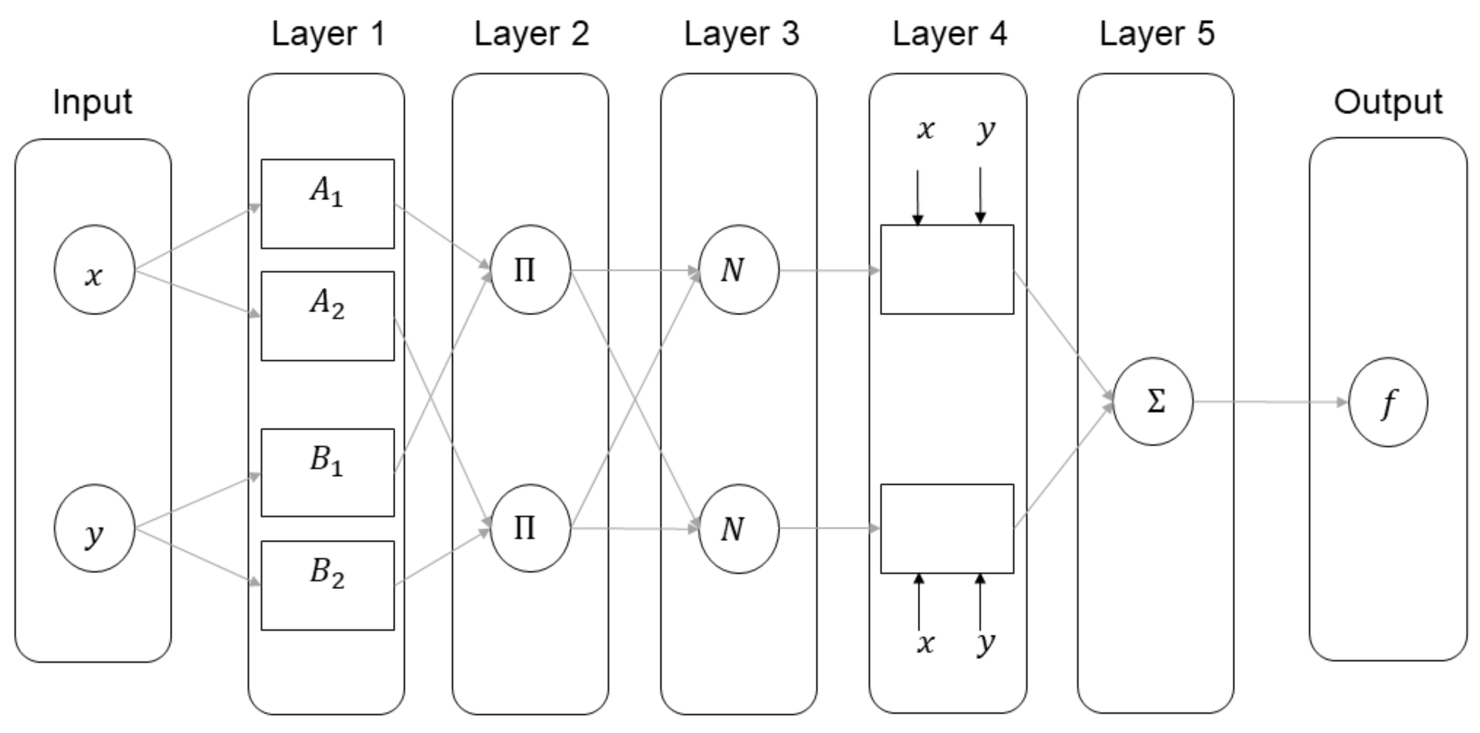
The ANFIS model is a multilayer feed-forward network that combines the ANN model and fuzzy logic based on the Takagi–Sugeno fuzzy inference system [46]. It is a powerful tool for hydrological forecasting because it integrates the advantages of both the ANN and fuzzy inference systems. The fuzzy reasoning system for a first-order Sugeno fuzzy model has the following two if-then rules:
  • Rule 1: if   x   is   A 1   and   y   is   B 1   then f 1 = p 1 x + q 1 y + r 1
  • Rule 2: if x is A 2 and y is B 2 then f 2 = p 2 x + q 2 y + r 2 where A 1 , A 2 and B 1 , B 2 are the membership functions of each input x and y , f 1 and f 2 are the output functions and p 1 ,   q 1 ,   r 1 and p 2 ,   q 2 ,   r 2   are linear parameters. The ANFIS model consists of five layers as shown in Figure 2.
Layer 1: The fuzzy membership grade for each node is generated by the fuzzy membership function (MF). An MF is an indicator function that defines how a point in the input space is mapped to a membership value between 0 to 1. The output of node i is defined in Equations (9) and (10):
Q 1 , i = μ A i ( x ) ,   i = 1 , 2
Q 1 , i = μ B i 2 ( y ) ,   i = 3 , 4 .
where x and y are the input for node i , and μ A i (or μ B i 2 ) is the degree of MF for a fuzzy set A i (or B i 2 ). The fuzzy set A i (or B i 2 ) is a linguistic label for a MF that could be given by appropriate functions such as Gaussian, generalized Bell shaped, trapezoidal shaped, and triangular shaped functions [1].
Layer 2: The incoming signals are multiplied to generate the output that represents the firing strength of the rules, as described in Equation (11).
Q 2 , i = w i = μ A i ( x ) × μ B i ( x ) ,   i = 1 , 2
Layer 3: The firming strength is normalized. The normalized firming strength for node i as described in Equation (12).
Q 3 , i = w i ¯ = w i ( w 1 + w 2 ) ,   i = 1 , 2
Layer 4: Consequent parameters { p i ,   q i ,   r i } at node i compute the contribution of the i th rule to the overall output. It can be described by Equation (13) using the output obtained from layer 3 ( w i ¯ ) .
Q 4 , i = w i ¯ f i = w i ¯ ( p i x + q i y + r i )
Layer 5: Finally, the overall output is calculated from a single node by summation of all rules as described in Equation (14).
Q 5 , i = i w i ¯ f i = i w i f i i w i
In this study, the ANFIS model used hybrid learning that was a combination of descent gradient for precedents and least squares estimation for consequents. The normalized Gaussian MF and Bell-shaped MF are popular, with the advantage of being smooth and nonzero at all points. The linguistic term of the normalized Gaussian MF and the Bell-shaped MF are given by Equations (15) and (16):
μ A i ( x ) = exp ( ( x c i ) 2 2 σ i 2 )
μ A i ( x ) = 1 1 + [ ( x c i a i ) 2 ] b i
where σ i ,   a i ,   b i , and   c i are the parameters of the membership function (i.e., c i and σ i are the center and width of the fuzzy set).

2.5. Random Forest (RF) Model

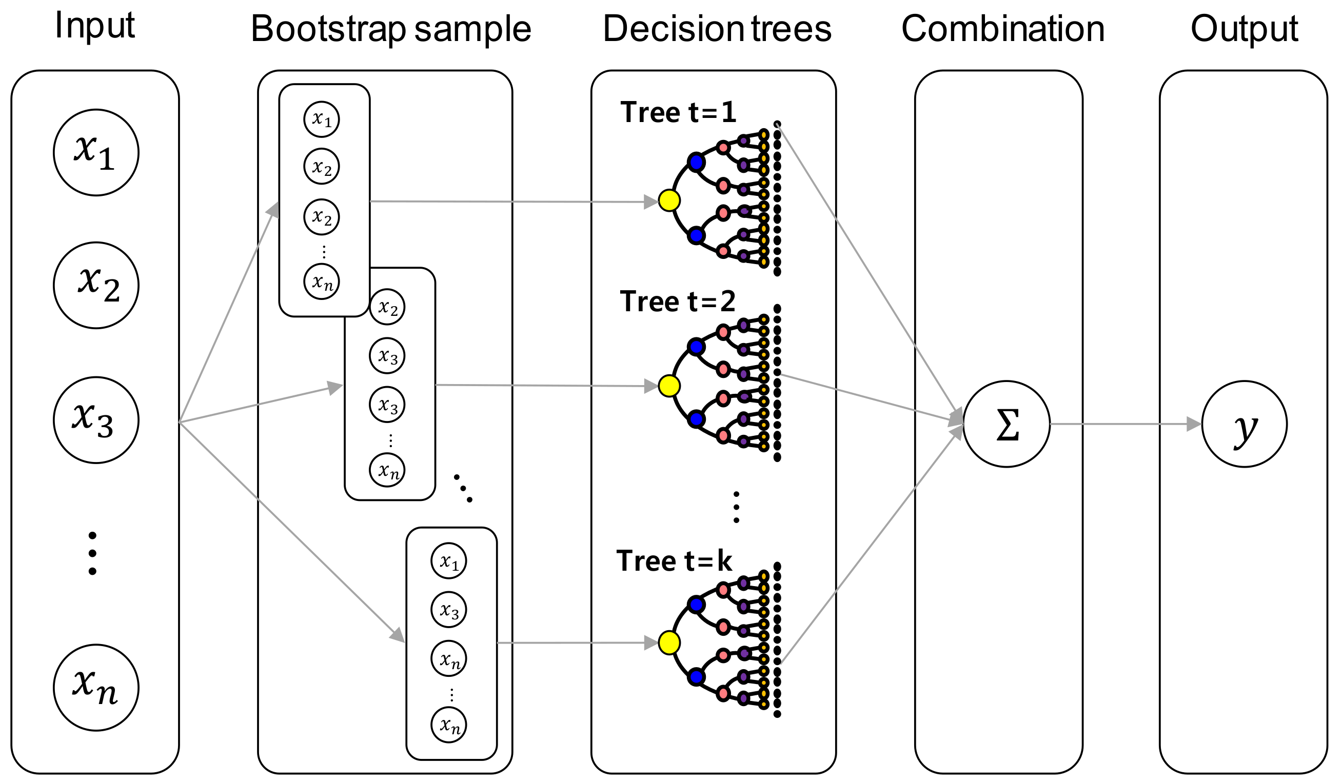
The RF model is a state-of-art machine learning technique which is a nonparametric white-box regression model [24]. For the regression, the RF model employs an ensemble-learning algorithm which operates by constructing a multitude of decision trees based on bootstrap samples from the training dataset. Unlike linear regression models, RF is the most robust technique for handling a combination of nonlinear interactions between the input variables and the output. The basic structure of the RF is shown in Figure 3.
The RF begins with many bootstrap samples that are randomly selected from the original input variables. A decision tree is built for each of the bootstrap samples. For each node of a decision tree, proper input variables are selected by binary partitioning. Finally, the forecasting result can be obtained by combining the results over all trees [47]. Therefore, three parameters need to be specified: (1) the number of trees; (2) number of variables in each node (default value is 5 for regression random forest); and (3) the number of input variables per node (default value is one third of the total number of variables).

3. Data and Study Area

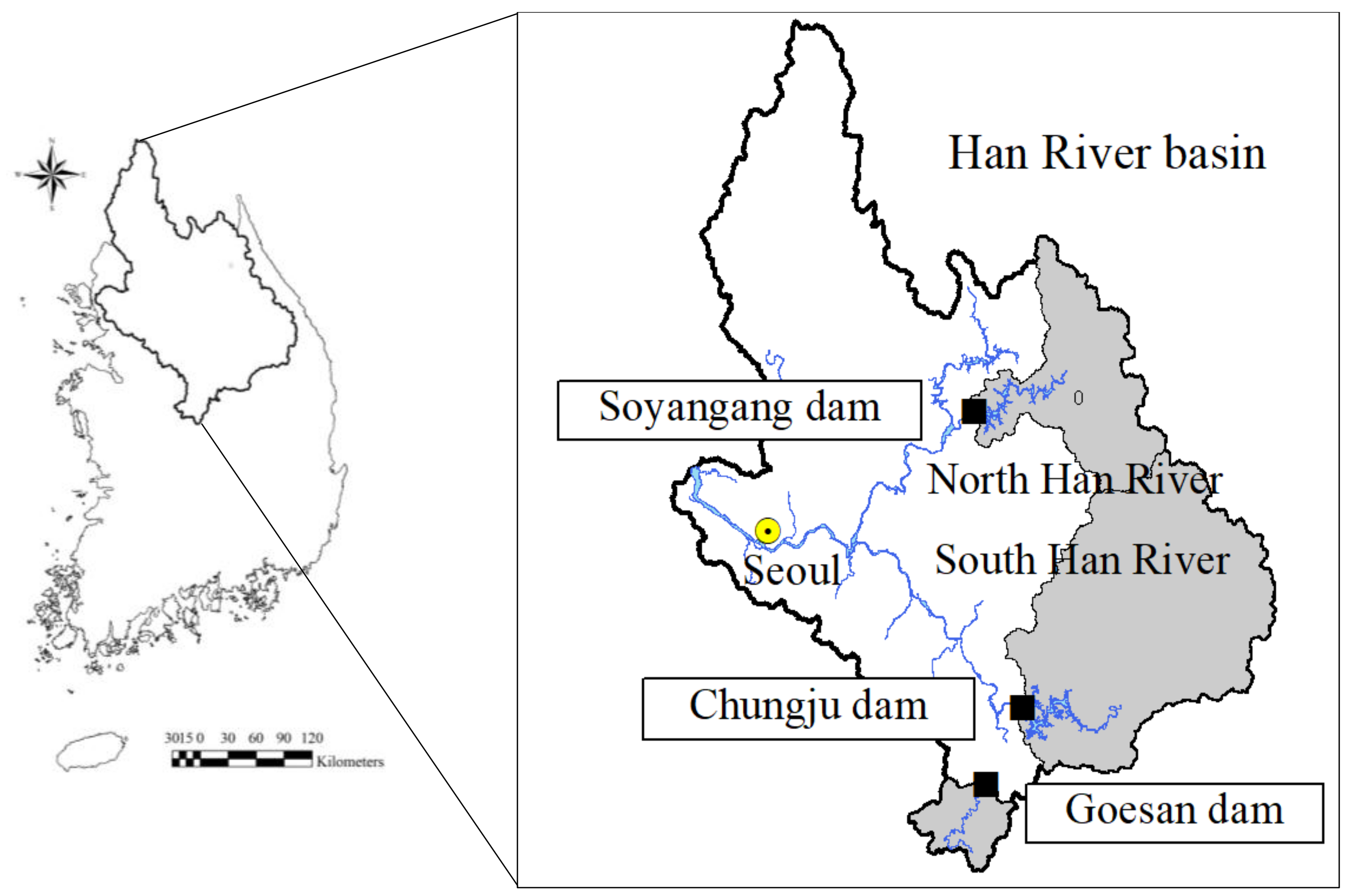
Monthly reservoir inflow in the SY, CJ, and GS dams was employed in this study. The three dams are located in the Han River basin, and they are totally separate reservoirs on different branches of the Han River. The three dams have only natural reservoir inflow that is not affected by artificial control in their upstream areas. The Han River basin in South Korea plays an important role in supplying water to the capital, Seoul, and other metropolitan cities. Therefore, the three dams should be carefully operated to provide effective long-term water management.
The SY dam is a multi-objective dam located in the upstream section of the North Han River, which has a basin area of 2783 km2. The CJ dam is the largest multi-objective dam in South Korea and is located on the South Han River, which has the basin area of 6705 km2. The GS dam is a small hydropower dam located on the Dalcheon, a tributary of the South Han River, with a basin area of 671 km2. There are seasonal characteristics to the inflow, with the monthly reservoir inflow concentrated during the flood season from June to September, since more than 70% of annual precipitation occurs in this season. The geographical locations of the three dams and basin areas are shown in Figure 4. Further detailed information about the three dams is presented in Table 1.
A total of 24 large-scale climate indices from the National Oceanic & Atmospheric Administration/Earth System Research Laboratory (NOAA/ESRL) were used in this study. The climate indices represent the atmospheric-oceanic circulation patterns, therefore, it can be possible to consider the impact of large-scale climate variability directly or indirectly on the monthly reservoir inflow series. Each index indicates an aspect of the geophysical system based on different measurements, and they are provided by the form of the monthly time series. Table 2 presents a list of the climate indices used in this study.

4. Input Variable Selection

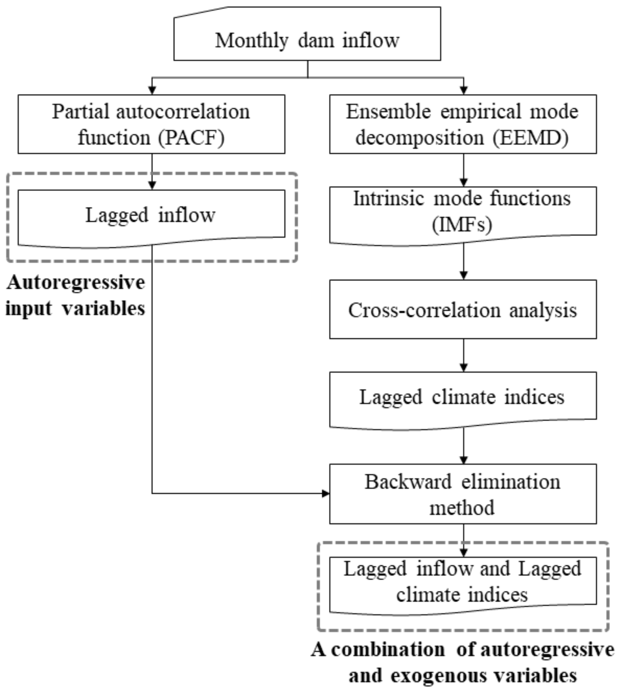
The time series and artificial intelligence models were conducted by two types of input variables to compare the impacts of the climate indices. The first type of input variable only includes the autoregressive variables (AR-) such as the lagged inflow. The lag time was determined by the PACF. The second type of input variable includes the combination of autoregressive and exogenous variables (ARX-) composed of lagged inflow and lagged climate indices. To select the candidate climate indices for the second type of input variables, the EEMD method was employed to the monthly reservoir inflow series. A finite number of decomposed components, which are the IMFs, were extracted by the EEMD. Cross-correlation analysis was performed between the IMFs and the climate indices considering lag times from 1 to 12 months. The lagged climate indices with the highest correlation coefficient with each IMF were selected as the candidate climate indices. Therefore, the candidate variables include: (1) the lagged inflow obtained via PACF; and (2) the lagged climate indices obtained via EEMD. Finally, the backward elimination method was performed on the candidate variables to select the second type of input variables. Figure 5 shows the procedure followed to select the two types of input variables. Detailed methodologies are explained in the subsections.

4.1. Partial Autocorrelation Function (PACF)

PACF is a statistic that measures the strength of relationships in a time series considering a time lag, after removing the presence of all other time lags. The range of PACF is between −1 and 1. In a PACF plot, it is able to identify the relationship between a time series and its lagged time series through the spikes and confidence intervals. For example, a significant spike at lag 12 in the PACF plot means that there is a strong correlation between a time series and the same time series with twelve intervals apart. PACF also provides useful information for selecting the autoregressive parameters in the time series models.

4.2. Ensemble Empirical Mode Decomposition (EEMD)

EMD has been recently introduced in the hydrology as an innovative analysis method to decompose statistically significant cycles and trends inherent in time series data [36,40,48]. EMD is a data-driven method that decomposes an original data series into a set of IMFs. IMFs indicate oscillatory modes that reflect the cycles and trends in the data series and should satisfy two conditions: (1) the number of extrema and zero crossings must either be equal or differ at most by one in the whole data series; (2) the mean value of the upper envelope defined by connecting all of the local maxima, and the lower envelope defined by connecting all of the local minima, must be zero at any point [47]. EEMD is a modified version of EMD proposed by Wu and Huang [49] to overcome the drawbacks of EMD due to the mode mixing problem. EEMD performs a sifting algorithm by adding an ensemble of white noise signals to the original data series, and the final result is obtained from the mean of the data series.
We will briefly introduce the sifting algorithm which is carried out to decompose a set of IMFs from an original data series y ( t ) , t = 1 , 2 , , n [36]. At first, the upper and lower envelopes are found by connecting the local maxima ( y u ( t ) ) and local minima y l ( t ) ) using a cubic spline method. Second, the mean value between the local maxima and local minima is calculated, i.e., y m e a n ( t ) = ( y u ( t ) + y l ( t ) ) / 2 . Third, the y m e a n ( t ) is extracted from the original time series y ( t ) , i.e., h ( t ) =   y ( t ) y m e a n ( t ) . If h ( t ) satisfies the two conditions of IMFs, then h ( t ) is the first IMF; else h ( t ) is treated as y ( t ) and the steps are repeated until h ( t ) becomes the IMF. Fourth, a new data series is defined by extracting the IMF from y ( t ) and repeating the steps until no more IMF can be extracted. The last IMF becomes the residue r ( t ) . Finally, y ( t ) is defined as the sum of the IMFs and the residue as follows:
y ( t ) = i = 1 k I M F i ( t ) + r ( t )
where k is the number of IMFs.

4.3. Cross-Correlation Analysis

Cross-correlation function is a measure of the strength of a linear correlation between two different time series considering a range of time lags. The range of the correlation coefficient (r) is between −1 and 1. If the two different time series are positively correlated, r is close to 1; if they are negatively correlated, r is close to −1; if they have no correlation, r is 0.

4.4. Backward Elimination Method

Backward elimination method is a kind of variable selection method beginning with all candidate input variables for a model. From the initially selected candidate input variables, the least significant variables are eliminated one by one until only one variable remains. The input variable showing the smallest contribution to the model performance is deleted at each step according to the model selection criteria. The relative importance of the input variable may be determined by removing the input variable [50]. The backward elimination method is useful for improving the model’s performance with an iterative procedure, although it requires significant computational time.

5. Application and Results

5.1. Model Input Variables

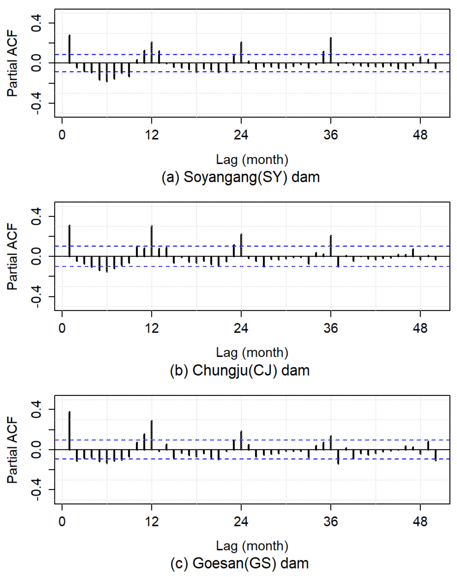
To determine the autoregressive variables, the PACF was used to identify the lag time of the monthly reservoir inflow series. Figure 6 shows the PACF of the three dams with 95% confidence intervals. At all three dams, the spikes are mainly prominent at 1, 12, 24, and 36 months (lag1, lag12, lag24, lag36; y t 1 ,     y t 12 , y t 24 ,   y t 36 ). Therefore, the first type of input variables for all the three dams includes the four cases of lagged inflows as shown in the second column of Table 3.
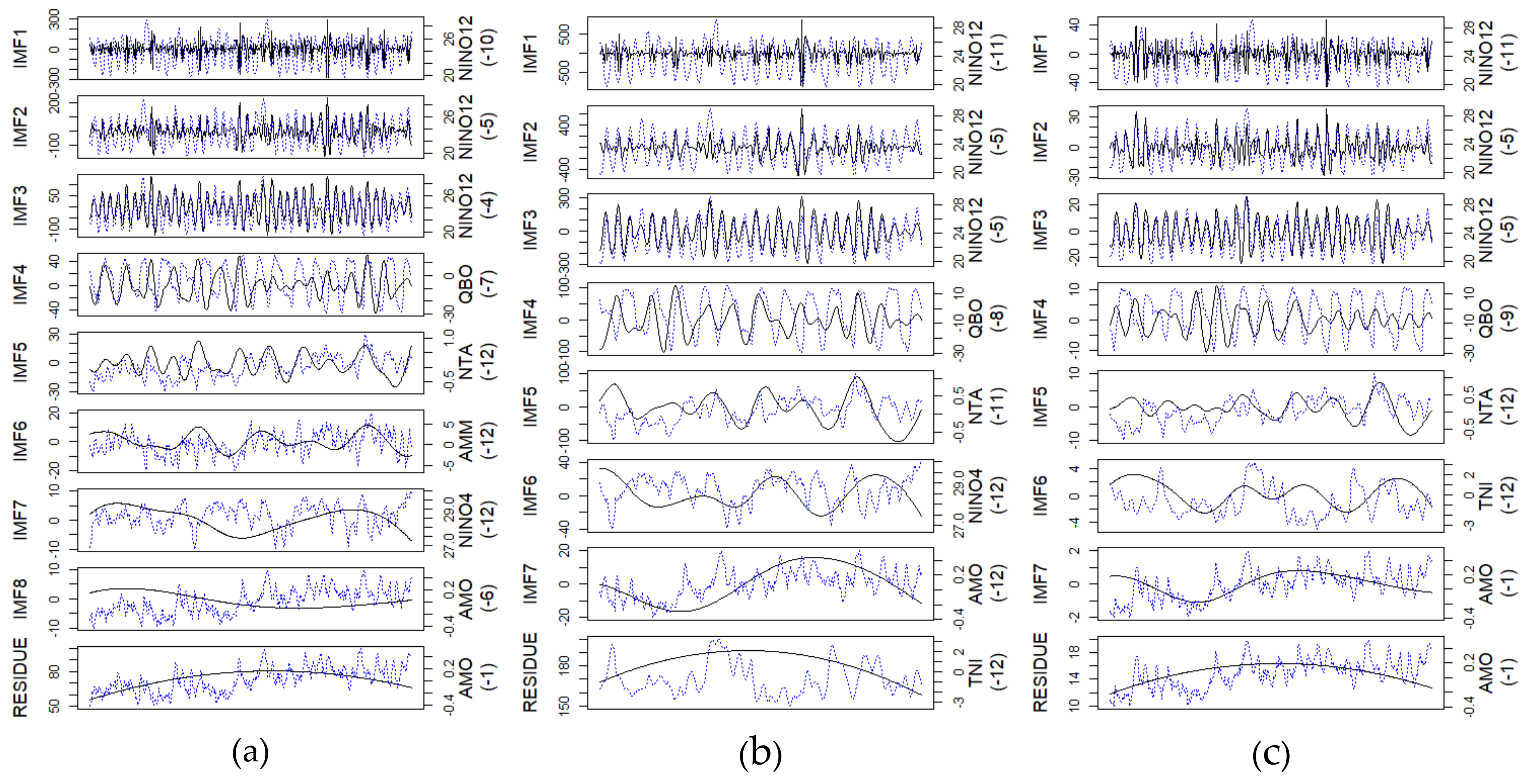
To determine the exogenous variables for the second type of input variables, the monthly reservoir inflow series was decomposed by EEMD to extract the IMFs. The IMFs indicate the different inherent frequencies of the reservoir inflow series. Lagged climate indices which have the highest correlation coefficient for each IMF were selected as the candidate exogenous variables. Figure 7 shows the IMFs (solid black line) of the three dams and the lagged climate indices which have the highest correlation coefficient for each IMF (blue dotted line). The reservoir inflow of the SY dam was decomposed into eight IMFs and a residue, and the reservoir inflow of the CJ and GS dams were decomposed into seven IMFs and a residue. For all three dams, the NINO12 index was mainly selected in the low-frequency IMF, the NTA and QBO indices were mainly selected in the middle frequency IMF, and the AMO index was mainly selected in the high-frequency IMF or residue. Table 4 shows the correlation coefficients (r) between the IMFs and the lagged climate indices in the SY, CJ, and GS dams. In the SY dam, the 4-month lagged NINO12 index had the highest correlation coefficient (r = 0.76) with the third IMF and the 6-month lagged AMO index has the second highest correlation coefficient (r = −0.57) with the eighth IMF. In the CJ dam, the 5-month lagged NINO12 index had the highest correlation coefficient (r = 0.75) with the third IMF, and the 12-month lagged AMO index had the second highest correlation coefficient (r = 0.49) with the seventh IMF. In the GS dam, the 5-month lagged NINO12 index had the highest and the second highest correlation coefficients (r = 0.75, r = 0.45) with the third and second IMFs, respectively. The 12-month lagged NTA index had the third highest correlation coefficient (r = −0.40) with the fifth IMF.
To determine the second type of input variables for each dam, the backward elimination method was applied to the candidate variables, including the lagged inflows and the lagged climate indices. The backward elimination method results were shown in the third column in Table 3, which are the second type of input variables for each dam composed of a combination of autoregressive and exogenous variables. Therefore, a total of seven, six, and five input variables were finally selected for the SY, CJ, and GS dams. Notably, the 36-month lagged inflow, lagged NINO12 index, and lagged AMO index were identically selected as the second type of input variables at all the three dams.

5.2. Model Parameters and Setting

A total of eight models including time series and artificial intelligence models with the two types of input variables (SARIMA, SARIMAX, AR-ANN, ARX-ANN, AR-ANFIS, ARX-ANFIS, AR-RF, and ARX-RF) were constructed. To calibrate and validate the time series models, the monthly reservoir inflow series was divided into train and test periods. The training period was set from the start of the data record to December 2012 and the test periods were set to the last four years (January 2013 to December 2016). In the artificial intelligence models, the monthly reservoir inflow series was divided into three parts, training, validation, and test periods to avoid overfitting problem. The training period was set from the start of the data record to December 2008 and the validation period was set to the next four years (January 2009 to December 2012). The test periods were set to the last four years (January 2013 to December 2016). Detailed descriptions of the model parameters and architectures are presented in the subsections.

5.2.1. SARIMA and SARIMAX Models

The SARIMA model is a conventional statistical model used to forecast future values. It is composed of autoregressive terms. The SARIMAX model, which is very similar to the SARIMA model, extends into the SARIMA model with an exogenous variable. Both the SARIMA and SARIMAX models consist of the parameters (p, d, q)(P, D, Q)[s]. In general, it is sufficient to consider up to two non-seasonal AR and MA parameters ( p , q ) and seasonal AR and MA parameters ( P , Q ) [51]. In this study, the SARIMA and SARIMAX models were composed of the non-seasonal AR and MA parameters ( p , q ) and the seasonal AR and MA parameters ( P , Q ) up to three (from 0 to 3) for more flexible model construction. Depending on the behavior of the reservoir inflow, non-seasonal and seasonal differencing orders were respectively set to 0 and 1 ( d = 0 ,   D = 1 ), and the seasonal periods were set to 12 ( s = 12 ) ) reflecting seasonality with 12-month intervals in the reservoir inflow (in Figure 5).
A total of 256 (4 × 1 × 4 × 4 × 1 × 4) SARIMA models were respectively constructed for the SY, CJ, and GS dams. The number of constructed SARIMAX models was the number of SARIMA models multiplied by the number of combination autoregressive and exogenous variables in Table 3, because the SARIMAX model is able to consider one exogenous variable. The rest of the parameters were identical to the structure of the SARIMA model. A total of 1792 (256 × 7), 1536 (256 × 6), 1280 (256 × 5) SARIMAX models were respectively constructed for the SY, CJ, and GS dams. The best SARIMA and SARIMAX models were selected based on the minimum Akaike information criterion (AIC) value, which is commonly used for model selection. Table 5 shows the parameters of best SARIMA and SARIMAX models for the SY, CJ, and GS dams. For both model types, the best models were selected when the non-seasonal parameters had little effect ( p = 0 ) . In addition, the lagged inflow was selected as the exogenous variable for the SARIMAX models for all the three dams.

5.2.2. ANN Models

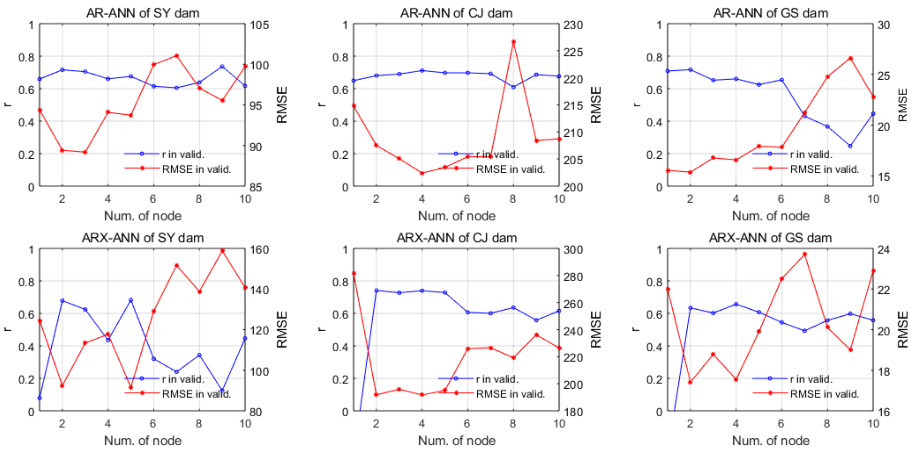
For the AR-ANN and ARX-ANN models, a number of hidden nodes ranging from 1 to 10 were considered in all three dams. The sigmoid activation function was used because of its superiority [4]. The optimal number of the hidden nodes for each dam was determined by considering the performance during the validation period. The correlation coefficient (r) and root mean square error (RMSE) of the AR-ANN and ARX-ANN models according to the number of the hidden nodes in the validation periods are shown in Figure 8. The optimal number of the hidden nodes was determined based on the highest r and the lowest RMSE. In cases of two criteria were different, the RMSE was preferred. Table 6 shows the optimal number of the hidden nodes of the AR-ANN and ARX-ANN models for the three dams.

5.2.3. ANFIS Models

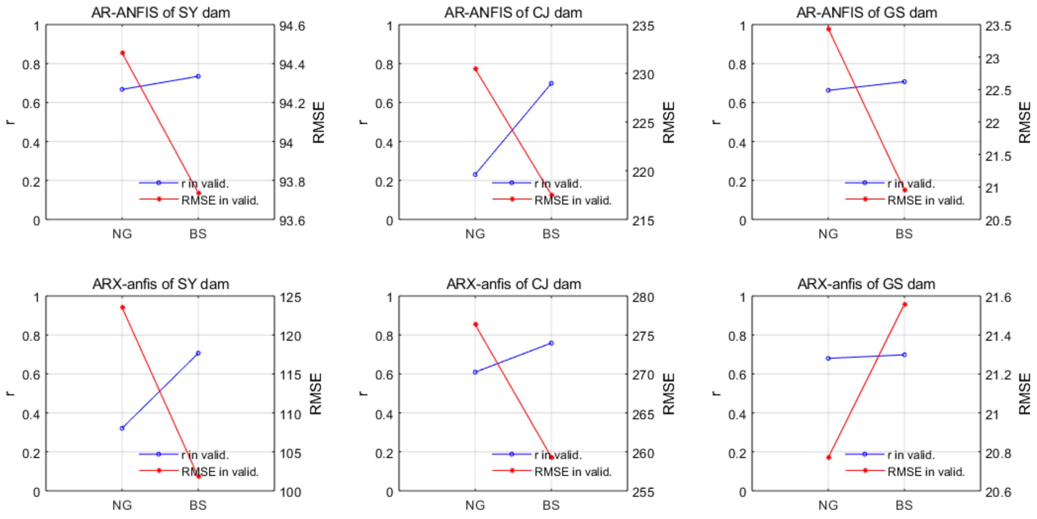
For the AR-ANFIS and ARX-ANFIS models, two MFs were built on the normalized Gaussian MF ( c i   = −5, σ i   = 2 and c i = + 5, σ i = 2) and Bell-shaped MF (a = 4, b = 1, c = −5 and a = 4, b = 1, c = +5), and 20 epochs based on trial and error [52]. The optimal MF was determined by considering the performance during the validation period. The correlation coefficient (r) and root mean square error (RMSE) of the AR-ANFIS and ARX-ANFIS models according to the MF in the validation periods are shown in Figure 9. The optimal MF was determined based on the highest r and the lowest RMSE. In cases where two criteria were different, the RMSE was preferred. For the AR-ANFIS model, there were eight input MFs and 16 rules in the three dams because there are four cases of lagged inflow in the autoregressive input variable set. For the ARX-ANFIS model, the number of input MFs according to the number of input nodes was 14, 12, and 10 for the SY, CJ, and GS dams, respectively. Therefore, the number of rules were 128, 64, and 32. Table 7 shows the optimal MF, the number of input MFs and rules of the AR-ANFIS and ARX-ANFIS models for the three dams.

5.2.4. RF Models

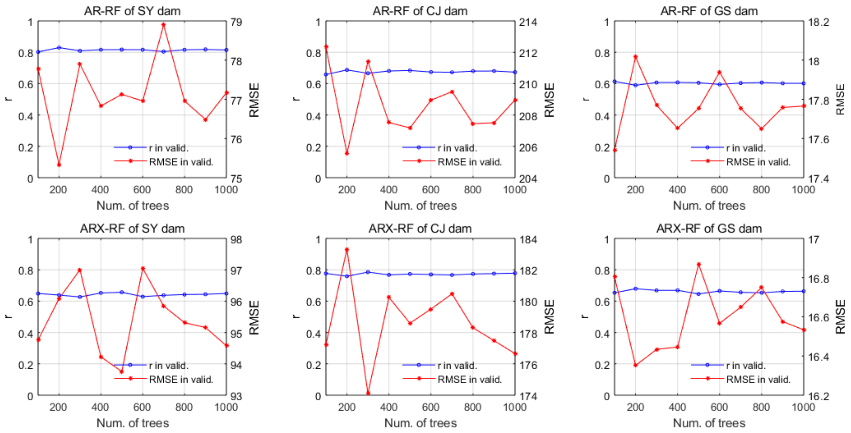
For the AR-RF and ARX-RF models, the number of trees ranging from 100 to 1000 (in 100 units) were considered in all the three dams. The optimal number of trees was determined by considering the performance during the validation period. The correlation coefficient (r) and root mean square error (RMSE) of the AR-RF and ARX-RF models according to the number of trees in the validation periods are shown in Figure 10. The optimal MF was determined based on the highest r and the lowest RMSE. In the case of two criteria were different, the RMSE was preferred. Table 8 shows the optimal number of trees of the AR-RF and ARX-RF models for the three dams.

5.3. Model Performance

Model performance can be evaluated based on different statistical measures. Two statistical criteria were used to estimate the model performance in this study. The correlation coefficient (r) is widely used to identify the linear relationship between observed and forecasted data. The value of r has a range of –1 to 1 that indicates either a negative or positive correlation. The root mean square error (RMSE) is used to measure the difference between observed and forecasted data. The value of RMSE indicates the magnitude of the error. The Nash–Sutcliffe Efficiency (NSE) is used to assess the predictive power of hydrological models. The value of NSE has a range from − to 1. The r, RMSE, NSE are defined in Equations (18), (19), and (20), respectively.
r = t = 1 T ( Y ( t ) Y ¯ ( t ) ) ( X ( t ) X ¯ ( t ) ) t = 1 T ( Y ( t ) Y ¯ ( t ) ) 2 t = 1 T ( X ( t ) X ¯ ( t ) ) 2
R M S E = 1 T t = 1 T ( Y ( t ) X ( t ) ) 2
N S E = 1 t = 1 T ( Y ( t ) X ( t ) ) 2 t = 1 T ( X ( t ) X ¯ ( t ) ) 2
where T is data length, Y ( t ) and X ( t ) are the forecasted and observed data series, and   Y ¯   ( t ) and   X ¯   ( t ) are the mean of the forecasted and observed data series, respectively.
The calculated r, RMSE, and NSE during the training, validation, and test periods of SARIMA, SARIMAX, AR-ANN, ARX-ANN, AR-ANFIS, ARX-ANFIS, AR-RF, and ARX-RF models for the SY, CJ, and GS dams were presented in Table 9. The underlined values indicate the best statistics among the employed models in the training, validation, and test periods. In the SY dam, the result shows that the ARX-RF and AR-RF models are very competitive and have good performance in the training and validation periods, respectively. On the other hand, in the test period, the AR-ANN or ARX-ANN models shows the best performance although it is slightly different according to the statistical criteria. In CJ dam, the ARX-RF model shows the best performance in the training and validation periods. On the other hand, the ARX-ANN model outperforms in the test period. In the GS dam, the ARX-RF model shows the best performance in the training period while the AR-ANN model shows the best performance in the validation period. The SARIMA and AR-RF models achieve the best performance in the test period depending on the statistical criteria. Overall, the ARX-RF model outperforms in the training period. Focusing on the test period, the ARX-ANN model generally provided better predictions, except for the GS dam. In summary, the time series model does not prove that the use of climate indices as an exogenous variable is more efficient. However, the use of climate indices generally tends to produce better performance in the ANN and RF models.
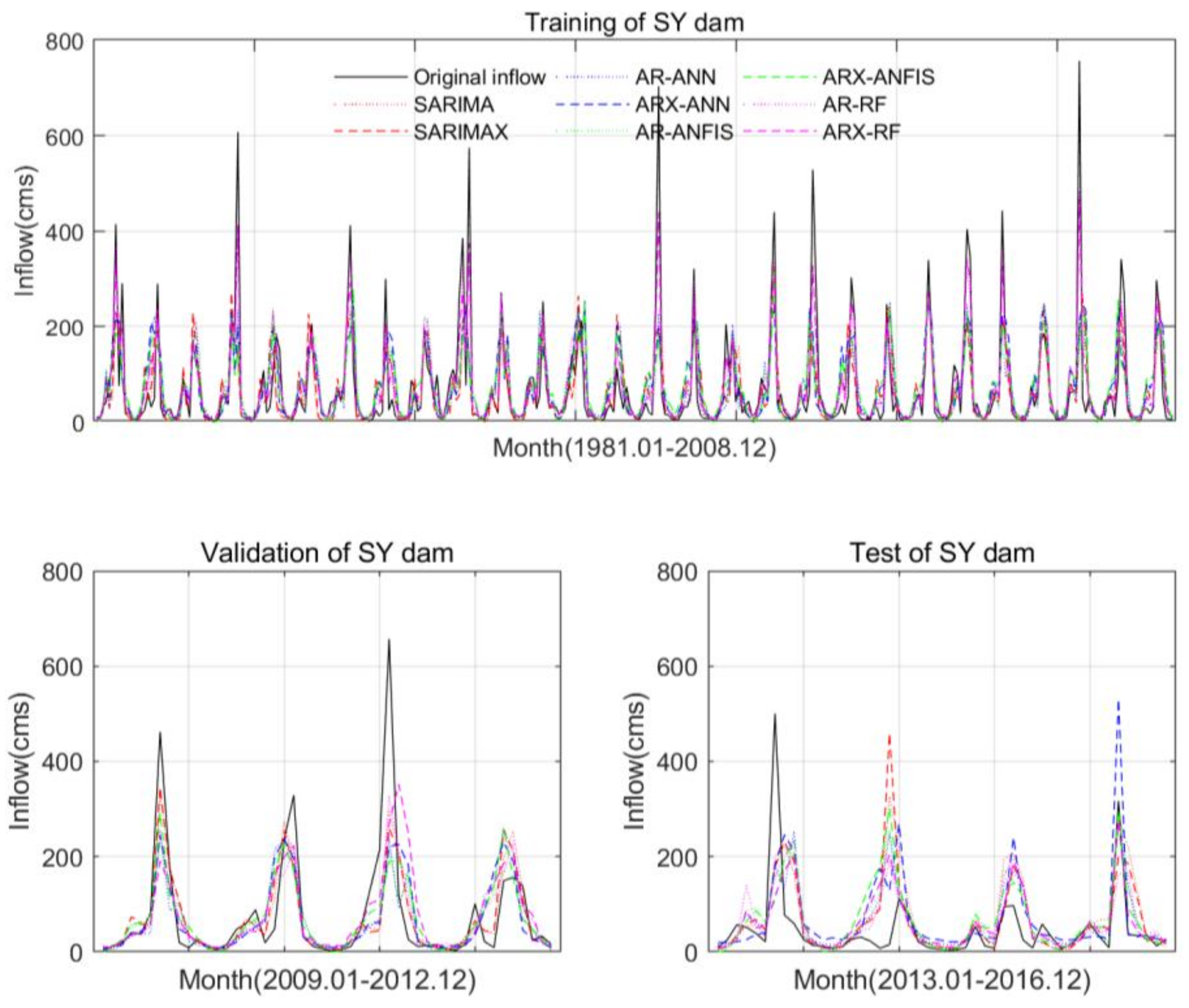
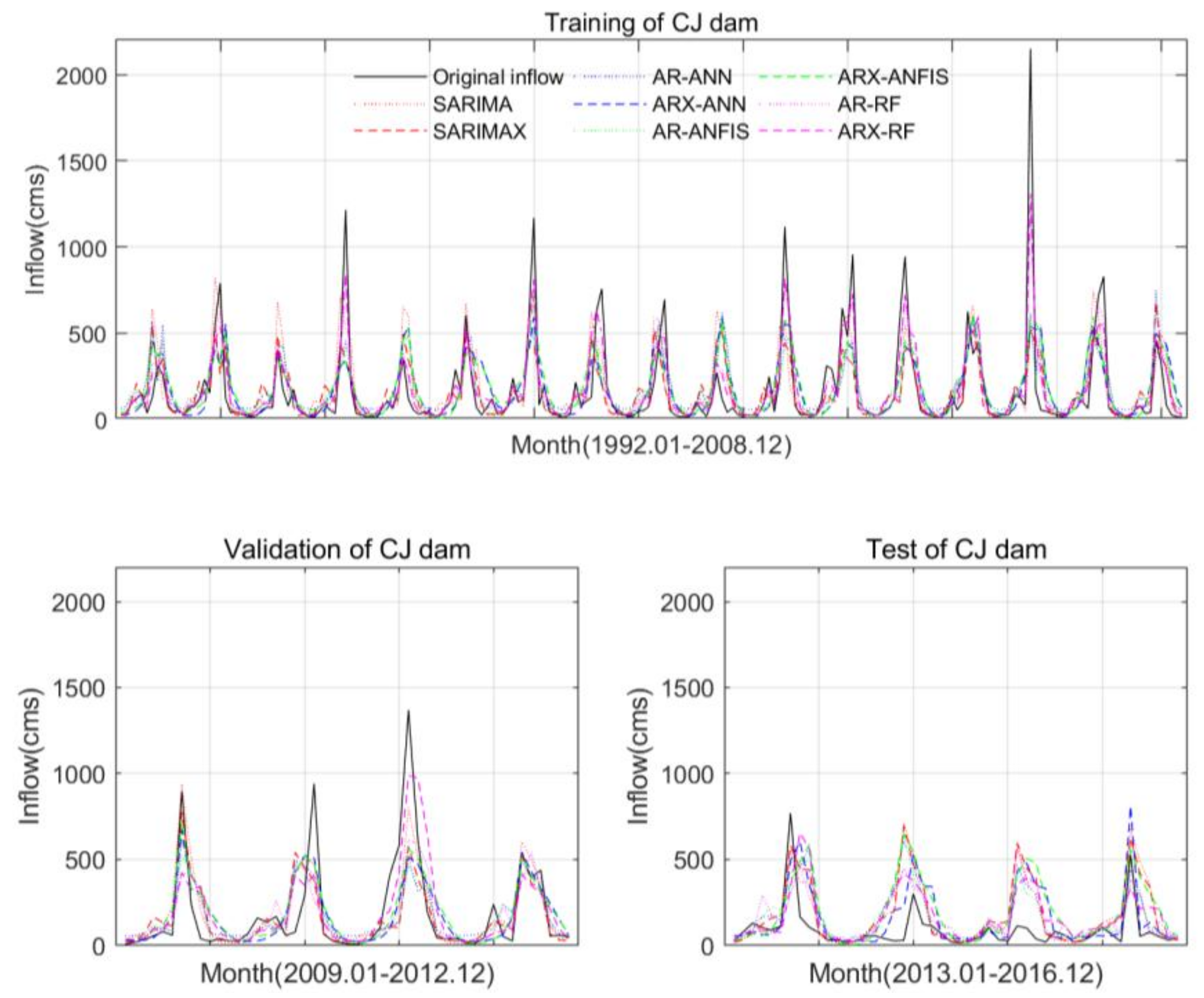
The reservoir inflow forecasting results from the SARIMA, SARIMAX, AR-ANN, ARX-ANN, AR-ANFIS, ARX-ANFIS, AR-RF, and ARX-RF models for the SY, CJ, and GS dams are shown in Figure 11, Figure 12 and Figure 13, respectively. The training periods for the SY, CJ, and GS dams were respectively started in 1981, 1992, and 1987 considering the order of the time series models. In Figure 11, Figure 12 and Figure 13, a part of forecasting results in the training period of the SARIMA and SARIMAX models were illustrated to the validation period. The general results of the time series models showed that they forecast only seasonal patterns even in both training, validation, and test periods. In addition, there were no significant differences between the SARIMA and SARIMAX models depending on the exogenous variables. The forecasted reservoir inflows of the SARIMA and SARIMAX models were very close, and were unable to forecast the extreme inflow during the flood season in both the training and test periods. This indicates the impact of the climate index was insufficient in the time series model. On the other hand, the exogenous variables have an impact on the performance of artificial intelligence models. The general results of the ARX-RF models showed that they forecast well not only seasonal patterns, but also peak flows during the flood season in the training and validation periods for all three dams. During the test period, the ARX-ANN model matched the seasonal patterns of inflow better than the other employed models, although it showed less accuracy in the volume. Although the ARX-ANN model showed lower forecasting performance in the training period than the ARX-RF model, the ARX-ANN model was able to make better forecasts of low and medium reservoir inflows than the ARX-RF model in the test period. By adding the validation period, we could avoid the overfitting problem. With regard to unsatisfactory performance in the test period captured by the NSE, this will be discussed further in the discussion section.

6. Discussion

In this study, the statistical methods (e.g., PACF and EEMD) were employed to select the two types of input variables including lagged inflow and lagged climate indices. The PACF for all three dams mainly resulted in prominent spikes at 1, 12, 24, and 36 months. The EEMD showed that the third IMF had the highest correlation coefficient with the four or five-month lagged NINO12 index and residues, and the last IMF also had a considerably high correlation coefficient with the 1- or 12-month lagged AMO index. It was found that the EEMD can obtain the inherent climate variability and long-term trend in the reservoir inflow. Therefore, the statistical relationship between the reservoir inflow and the climate indices can be deeply examined through EEMD.
From the results of the backward elimination method, the 36-month lagged inflow, NINO12 index, and the AMO index were selected as a combination of autoregressive and exogenous variables for the three dams in Table 3. Consequently, we found that the three variables mainly affect reservoir inflow and play an important role as input variables. This finding supported the results obtained by Kim et al. [41] that identified the four-month lagged NINO12 and AMO indices as effective indicators for long-term precipitation in South Korea, as the precipitation is causally related to reservoir inflow. In addition, this result also agrees with previous studies [36,38,40,53,54] that showed the IMFs identified through EEMD include the cyclical variabilities and overall trends of time series data.
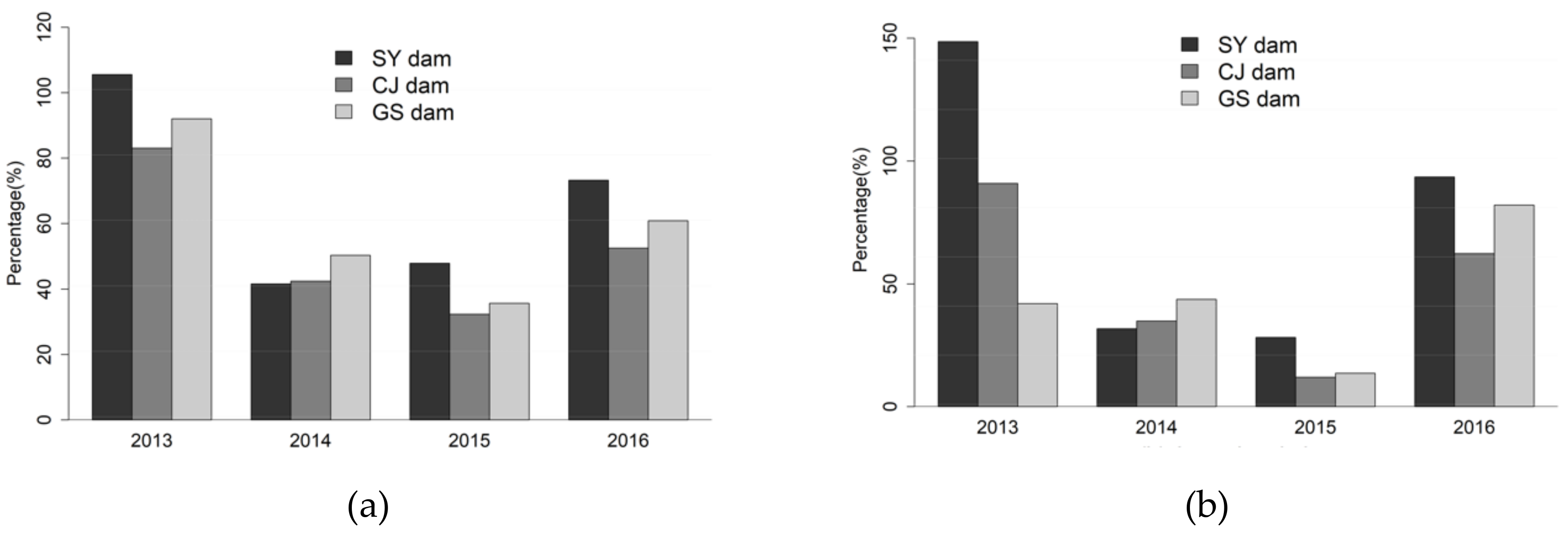
The comparison of model performance proved that the impact of the climate index was insufficient in the time series model while the exogenous variables have an impact on the performance of artificial intelligence models. The ARX-RF models generally forecasted well not only seasonal patterns, but also peak flows during the flood season in the training and validation periods for all the three dams. On the other hand, the ARX-ANN model generally showed better performance in the test period by matching the seasonal patterns of inflow although it showed less accuracy in the volume. However, the unsatisfactory performance in the test period captured by the NSE was due to severe weather conditions that rarely occurred in the observation period. To further understand the model performance under extreme weather conditions, the test period (2013–2016) was divided into each year, and the inflow characteristics were examined in each year. Figure 14(a) shows the percentage of the inflow rate of the year compared to the mean annual inflow in the 2013 to 2016 years for each dam. Figure 14(b) shows the percentage of the variation rate of the year compared to the mean annual variation in the 2013 to 2016 years for each dam. For example, the percentage of the inflow rate of 2013 year is calculated by (the mean annual inflow in 2013/the mean annual inflow in the training period) × 100(%). The percentage of the variation rate is calculated in the same way.
Notably, extreme weather conditions occurred during the test period. The dam inflow in 2013 approximated the mean annual inflow, however, there was a large difference in annual variation compared to the mean variation for the three dams. The annual inflow of the three dams was less than half the mean annual inflow in 2014 and decreased further in 2015 because a severe drought occurred in these two years. Due to the severe drought, the annual variation in inflow was also lower than average and there was minor difference in variation between the three dams. Inflow slightly increased in 2016 reaching half the mean annual inflow. In this study, the years of test period are defined as an ordinary year (2013), a drought year (2014), a severe drought year (2015), and a restored year (2016). Table 10 presents the model performances in the 2013 to 2016 years for the three dams.
In the ordinary year (2013), the time series models generally showed better performance than the artificial intelligence models. When the percentage of the annual variation was similar or smaller than the mean annual variation, such as was observed in GS dam, the AR-RF model generally showed the best forecasting accuracy based on both the RMSE and NSE. There were no significant differences according to the exogenous variables.
In the drought year (2014), the time series model performance was significantly poorer than during the ordinary year. The forecasting accuracy of the ARX-ANN and AR-RF models was generally better than other models based on the r and RMSE. The NSE captured poor performance at all dams because the mean inflows had been lowered due to drought effects. This result indicates that exogenous variables in the ANN model can improve forecasting accuracy during drought years, although there are limitations to forecasting the inflow volume.
In the severe drought year (2015), when the annual inflow was close to 50% of the mean annual inflow such as in the SY dam, all models showed improved forecasting accuracy. The ARX-ANFIS model showed the best forecasting accuracy based on the RMSE and NSE while the AR-RF model showed the best forecasting accuracy based on the r. However, when the annual inflow was lower than 40% of the mean annual inflow such as in the CJ and GS dams, the forecasting accuracy showed the worst performance, especially based on the NSE. This result shows a limitation of the use of exogenous variables in forecasting extreme weather conditions such as severe droughts, since the lagged climate indices mainly reflect the inherent climate variabilities and long-term trends.
In the restored year (2016), the ARX-RF and ARX-ANN models usually had the best forecasting accuracy for the SY and GS dams. Although the AR-ANN model showed better forecasting accuracy than the ARX-ANN model for the CJ dam based on the RMSE and NSE, the ARX-ANN model showed best forecasting accuracy based on the r. This result implies that the exogenous variables in the artificial intelligence models play an important role in forecasting accuracy under the restored climate conditions.
It was observed that the time series models have quite similarly forecasted inflow in the test period for the three dams. Mainly in the drought and severe drought years, the results generally described a limitation of the time series and artificial intelligence models, because the models are based on the observed data series. They only forecasted ordinary patterns of the observed inflow series. The r of the time series models decreased in the drought and severe drought years and slightly increased in the restored year because the time series models maintain seasonal patterns regardless of changing weather characteristics. The model performance in the artificial intelligence models was slightly different depending on the dam, period, climate conditions, and input variables. This also implies a difficulty to forecast events that have not been previously observed, although the model was trained very well. Among them, the AR-RF and ARX-ANN models generally showed better forecasting accuracy under drought conditions in our case study. Therefore, we can conclude that the use of artificial intelligence model and climate indices as exogenous variables has the potential to provide a suitable forecasting performance under the changing climatic conditions.
Reservoir inflow forecasting is still a challenge for reservoir managers all over the world. Reservoir managers should strive to operate the reservoir considering the various results from statistical, artificial intelligence, and dynamic models. In light of this decision-making, our study can be useful in making decisions for reservoir operation, because they showed good performance in forecasting inflow patterns by using lagged inflows and lagged climate indices. Finally, we also agree with Zhang et al. [55] that future studies should be ongoing by applying a new type of machine learning algorithm, i.e., deep learning, derived from the ANN model.

7. Conclusions

In this study, the use of large-scale climatic indices as exogenous input variables to hydrologic forecasting models was considered to reflect climate variability due to climate change. To do this, a total of eight models including time series and artificial intelligence models (SARIMA, SARIMAX, AR-ANN, ARX-ANN, AR-ANFIS, ARX-ANFIS, AR-RF, and ARX-RF) were applied to monthly reservoir inflow forecasting. The results of this study led to the following conclusions:
(1) For input variable selection, the PACF and EEMD can be used to find lagged inflow and lagged climate indices that have a significant relationship with dam inflow. As a result, four lagged inflows (lag1, lag12, lag24, lag36) were selected as the autoregressive variables, and the 36-month lagged inflow, the lagged NINO12 index, and the lagged AMO index were commonly selected as the combinations of autoregressive and exogenous variables for the three dams. Therefore, the procedure for input variable selection using the PACF, EEMD, cross-correlation analysis, and backward elimination in this study is a suitable method for input variable selection.
(2) The ARX-RF model generally showed the highest forecasting accuracy in the training period, which proves that a combination of autoregressive and exogenous variables is useful for constructing an RF model for the three dams. In the test period, the ARX-ANN model generally showed the highest forecasting accuracy by capturing the seasonal patterns of reservoir inflow well, although there are limitations to its ability to accurately forecast inflow volume.
(3) The model performance in the test period (from 2013 to 2016) was examined according to the inflow characteristics of each year. The inflow of the three dams maintained the seasonal patterns in 2013. Drought occurred in 2014, and it worsened in 2015. The ordinary pattern was slightly restored in 2016. Although the model performance was not consistent in each year of the test period, the ARX-ANN and the AR-RF models generally matched the seasonal patterns well, especially during the drought and restored years.
Based on this study, the results prove that the use of large-scale climate indices as exogenous variables has the potential to provide more efficient forecasting performance for water resource management and planning. Furthermore, there is a possibility to provide better forecasting results by using a state-of-art artificial intelligence models such as RF. Future studies should be required to identify the best forecasting models through many applications considering local weather conditions and inflow characteristics under the changing climate conditions for effective water management and planning.

Author Contributions

Conceptualization, T.K. and J.-Y.S.; Data curation, S.K.; Formal analysis, H.K.; Funding acquisition, J.-H.H.; Investigation, T.K. and H.K.; Methodology, T.K. and J.-Y.S.; Supervision, J.-H.H.; Visualization, H.K.; Writing–original draft, T.K.; Writing–review & editing, J.-H.H.

Funding

This research was supported by a grant(2017-MOIS31-001) from Fundamental Technology Development Program for Extreme Disaster Response funded by Korean Ministry of Interior and Safety(MOIS).

Acknowledgments

This research was conducted under the Development of long-term inflow forecasting technology and construction of water supply system (2nd year) supported by K-Water.

Conflicts of Interest

The authors declare no conflict of interest.

References

  1. Wang, W.-C.; Chau, K.-W.; Cheng, C.-T.; Qiu, L. A comparison of performance of several artificial intelligence methods for forecasting monthly discharge time series. J. Hydrol. 2009, 374, 294–306. [Google Scholar] [CrossRef] [Green Version]
  2. Wang, Y.; Guo, S.-L.; Chen, H.; Zhou, Y.-L. Comparative study of monthly inflow prediction methods for the Three Gorges Reservoir. Stoch. Environ. Res. Risk Assess. 2014, 28, 555–570. [Google Scholar] [CrossRef]
  3. Wang, W.C.; Chau, K.W.; Xu, D.M.; Chen, X.Y. Improving forecasting accuracy of annual runoff time series using ARIMA based on EEMD decomposition. Water Resour. Manag. 2015, 29, 2655–2675. [Google Scholar] [CrossRef]
  4. Valipour, M.; Banihabib, E.B.; Behbahani, S.M.R. Comparison of the ARMA, ARIMA, and the autoregressive artificial neural network models in forecasting the monthly inflow of Dez dam reservoir. J. Hydrol. 2013, 476, 433–441. [Google Scholar] [CrossRef]
  5. Awan, J.A.; Bae, D.-H. Improving ANFIS Based Model for Long-term Dam Inflow Prediction by Incorporating Monthly Rainfall Forecasts. Water Resour. Manag. 2014, 28, 1185–1199. [Google Scholar] [CrossRef]
  6. Kalteh, A.M. Wavelet Genetic Algorithm-Support Vector Regression (Wavelet GA-SVR) for Monthly Flow Forecasting. Water Resour. Manag. 2015, 29, 1283–1293. [Google Scholar] [CrossRef]
  7. Kisi, O. Streamflow Forecasting and Estimation Using Least Square Support Vector Regression and Adaptive Neuro-Fuzzy Embedded Fuzzy c-means Clustering. Water Resour. Manag. 2015, 29, 5109–5127. [Google Scholar] [CrossRef]
  8. Li, C.; Bai, Y.; Zeng, B. Deep Feature Learning Architectures for Daily Reservoir Inflow Forecasting. Water Resour. Manag. 2016, 30, 5145–5161. [Google Scholar] [CrossRef]
  9. Moeeni, H.; Bonakdari, H.; Ebtehai, I. Integrated SARIMA with Neuro-Fuzzy Systems and Neural Networks for Monthly Inflow Prediction. Water Resour. Manag. 2017, 31, 2141–2156. [Google Scholar] [CrossRef]
  10. Box, G.E.P.; Jenkins, G.M. Time Series Analysis Forecasting and Control; Holden-Day: San Francisco, CA, USA, 1970. [Google Scholar]
  11. Carlson, R.F.; MacCormick, A.J.A.; Watts, D.G. Application of linear random models to four annual streamflow series. Water Resour. Res. 1970, 6, 1070–1078. [Google Scholar] [CrossRef]
  12. Salas, J.D.; Tabios, G.Q.; Bartolini, P. Approaches to multivariate modeling of water resources time series. J. Am. Water Resour. Assoc. 1985, 21, 683–708. [Google Scholar] [CrossRef]
  13. Burlando, P.; Rosso, R.; Cadavid, L.G.; Salas, J.D. Forecasting of short-term rainfall using ARMA models. J. Hydrol. 1993, 144, 193–211. [Google Scholar] [CrossRef]
  14. Hipel, K.W.; McLeod, A.I. Time Series Modelling of Water Resources and Environmental Systems; Elsevier: Amsterdam, The Netherlands, 1994. [Google Scholar]
  15. Mohan, S.; Vedula, S. Multiplicative seasonal ARIMA model for longterm forecasting of inflows. Water Resour. Manag. 1995, 9, 115–126. [Google Scholar] [CrossRef]
  16. Papamichail, D.M.; Georgiou, P.E. Seasonal ARIMA inflow models for reservoir sizing. J. Am. Water Resour. Assoc. 2001, 37, 877–885. [Google Scholar] [CrossRef]
  17. Campolo, M.; Soldati, A.; Andreussi, P. Artificial neural network approach to flood forecasting in the River Arno. Hydrol. Sci. J. 2003, 48, 381–398. [Google Scholar] [CrossRef] [Green Version]
  18. Cheng, C.T.; Lin, J.Y.; Sun, Y.G.; Chau, K. Long-Term Prediction of Discharges in Manwan Hydropower Using Adaptive-Network-Based Fuzzy Inference Systems Models; Advances in Natural Computation; Springer: Berlin, Germany, 2005. [Google Scholar]
  19. Jain, A.; Kumar, A.M. Hybrid neural network models for hydrologic time series forecasting. Appl. Soft Comput. 2007, 7, 585–592. [Google Scholar] [CrossRef]
  20. Firat, M.; Gungör, M. Hydrological time-series modelling using an adaptive neuro-fuzzy inference system. Hydrol. Process. 2008, 22, 2122–2132. [Google Scholar] [CrossRef]
  21. Trichakis, I.; Nikolos, I.; Karatzas, G.P. Comparison of bootstrap confidence intervals for an ANN model of a karstic aquifer response. Hydrol. Process. 2011, 25, 2827–2836. [Google Scholar] [CrossRef]
  22. He, X.; Guan, H.; Zhang, X.; Simmons, C.T. A wavelet-based multiple linear regression model for forecasting monthly rainfall. Int. J. Climatol. 2014, 34, 1898–1912. [Google Scholar] [CrossRef]
  23. Nawaz, N.; Harun, S.; Talei, A. Application of Adaptive Network-Based Fuzzy Inference System (ANFIS) for River Stage Prediction in a Tropical Catchment. Appl. Mech. Mater. 2015, 735, 195–199. [Google Scholar] [CrossRef]
  24. Breiman, L. Random forest. Mach. Learn. 2001, 45, 5–32. [Google Scholar] [CrossRef]
  25. Yang, T.; Gao, X.; Sorooshian, S.; Li, X. Simulating California reservoir operation using the classification and regression-tree algorithm combined with a shuffled cross-validation scheme. Water Resour. Res. 2016, 52, 1626–1651. [Google Scholar] [CrossRef]
  26. Yang, T.; Asanjan, A.A.; Welles, E.; Gao, X.; Sorooshian, S.; Liu, X. Developing reservoir monthly inflow forecasts using artificial intelligence and climate phenomenon information. Water Rosour. Res. 2017, 53, 2786–2812. [Google Scholar] [CrossRef]
  27. Ahmed, J.A.; Sarma, A.K. Artificial neural network model for synthetic streamflow generation. Water Resour. Manag. 2007, 21, 1015–1029. [Google Scholar] [CrossRef]
  28. Noori, R.; Hoshyaripour, G.; Ashrafi, K.; Araabi, B.N. Uncertainty analysis of developed ANN and ANFIS models in prediction of carbon monoxide daily concentration. Atmos. Environ. 2010, 44, 476–482. [Google Scholar] [CrossRef]
  29. Valipour, M. Long-term runoff study using SARIMA and ARIMA models in the United States. Meteorol. Appl. 2015, 22, 592–598. [Google Scholar] [CrossRef] [Green Version]
  30. Emamgholizadeh, S.; Moslemi, K.; Karami, G. Prediction the groundwater level of Bastam Plain (Iran) by artificial neural network (ANN) and adaptive neuro fuzzy inference system (ANFIS). Water Resour. Manag. 2014, 28, 5433–5446. [Google Scholar] [CrossRef]
  31. Kashid, S.S.; Ghosh, S.; Maity, R. Streamflow prediction using multi-site rainfall obtained from hydroclimatic teleconnection. J. Hydrol. 2010, 395, 23–38. [Google Scholar] [CrossRef]
  32. Schepen, A.; Wang, Q.J.; Robertson, D. Evidence for using lagged climate indices to forecast Australian seasonal rainfall. J. Clim. 2012, 25, 1230–1246. [Google Scholar] [CrossRef]
  33. Mekanik, F.; Imteaz, M.A.; Gato-Trinidad, S.; Elmahdi, A. Multiple regression and artificial neural network for long-term rainfall forecasting using large scale climate modes. J. Hydrol. 2013, 503, 11–21. [Google Scholar] [CrossRef]
  34. Abbot, J.; Marohasy, J. Input selection and optimisation for monthly rainfall forecasting in Queensland, Australia, using artificial neural networks. Atmos. Res. 2014, 138, 166–178. [Google Scholar] [CrossRef]
  35. Li, J.; Liu, X.; Chen, F. Evaluation of nonstationarity in annual maximum flood series and the associations with large-scale climate patterns and human activities. Water Resour. Manag. 2015, 29, 1653–1668. [Google Scholar] [CrossRef]
  36. Wu, Z.; Huang, N.E.; Long, S.R.; Peng, C.K. On the trend, detrending, and variability of nonlinear and nonstationary time series. Proc. Natl. Acad. Sci. USA 2007, 104, 14889–14894. [Google Scholar] [CrossRef] [Green Version]
  37. Lee, T.; Ouarda, T.B.M.J. Long-term prediction of precipitation and hydrologic extremes with nonstationary oscillation processes. J. Geophys. Res. Atmos. 2010, 115, D13107. [Google Scholar] [CrossRef]
  38. Breaker, L.C.; Ruzmaikin, A. The 154-year record of sea level at San Francisco: Extracting the long-term trend, recent changes, and other tidbits. Clim. Dyn. 2011, 36, 545–559. [Google Scholar] [CrossRef]
  39. Shi, F.; Yang, B.; Gunten, L.; Qin, C.; Wang, Z. Ensemble empirical mode decomposition for tree-ring climate reconstructions. Theor. Appl. Climatol. 2012, 109, 233–243. [Google Scholar] [CrossRef]
  40. Castino, F.; Bookhagen, B.; Strecker, M.R. Oscillations and trends of river discharge in the southern Central Andes and linkages with climate variability. J. Hydrol. 2017, 555, 108–124. [Google Scholar] [CrossRef]
  41. Kim, T.; Shin, J.-Y.; Kim, S.; Heo, J.-H. Identification of relationships between climate indices and long-term precipitation in South Korea using ensemble empirical mode decomposition. J. Hydrol. 2018, 557, 726–739. [Google Scholar] [CrossRef]
  42. Yu, X.; Zhang, X.; Qin, H. A Data-driven Model Based on Fourier Transform and Support Vector Regression for Monthly Reservoir Inflow Forecasting. J. Hydro-Environ. Res. 2018, 18, 12–24. [Google Scholar] [CrossRef]
  43. Jalalkamali, A.; Moradi, M.; Moradi, N. Application of several artificial intelligence models and ARIMAX model for forecasting drought using the Standardized Precipitation Index. Int. J. Environ. Sci. Technol. 2015, 12, 1201–1210. [Google Scholar] [CrossRef]
  44. Yang, T.; Asanjan, A.A.; Faridzad, M.; Hayatbini, N.; Gao, X.; Sorooshian, S. An enhanced artificial neural network with a shuffled complex evolutionary global optimization with principal component analysis. Inform. Sci. 2017, 418–419, 302–316. [Google Scholar] [CrossRef]
  45. Avarideh, F. Application of Hydro-Informatics in Sediment Transport. Ph.D. Thesis, Amirkabir University of Technology, Tehran, Iran, 2012. [Google Scholar]
  46. Jang, J.S.R. ANFIS: Adaptive-Network-Based Fuzzy Inference System. IEEE Trans. Syst. Man. Cybern. 1993, 23, 665–685. [Google Scholar] [CrossRef]
  47. Wang, L.; Zhou, X.; Zhu, X.; Dong, Z.; Guo, W. Estimation of biomass in wheat using random forest regression algorithm and remote sensing data. Crop J. 2016, 4, 212–219. [Google Scholar] [CrossRef] [Green Version]
  48. Huang, N.E.; Shen, Z.; Long, S.R.; Wu, M.C.; Shih, H.H.; Zheng, Q.; Yen, N.C.; Tung, C.C.; Liu, H.H. The empirical mode decomposition method and the Hilbert spectrum for non-stationary time series analysis. Proc. Math. Phys. Eng. Sci. 1998, 354, 903–995. [Google Scholar] [CrossRef]
  49. Wu, Z.; Huang, N.E. Ensemble empirical mode decomposition: A noise-assisted data analysis method. Adv. Adapt. Data Anal. 2009, 1, 1–41. [Google Scholar] [CrossRef]
  50. May, R.; Dandy, G.; Maier, H. Review of Input Variable Selection Methods for Artificial Neural Networks. In Artificial Neural Networks-Methodological Advances and Biomedical Applications; Kenji, S., Ed.; InTechOpen: London, UK, 2011; ISBN 978-953-307-243-2. [Google Scholar] [Green Version]
  51. Cryer, J.D.; Chan, K.S. Time Series Analysis with Applications in R, 2nd ed.; Springer: New York, NY, USA, 2008; ISBN 978-0-387-75959-3. [Google Scholar]
  52. Sgurev, V.; Yager, R.R.; Kacprzyk, J.; Jotsov, V. Innovative Issues in Intelligent Systems; Springer: Cham, Switzerland, 2016; ISBN 978-3-319-27267-2. [Google Scholar]
  53. Lee, T.; Ouarda, T.B.M.J. Stochastic simulation of nonstationary oscillation hydro-climatic processes using empirical mode decomposition. Water Resour. Res. 2012, 48, W02514. [Google Scholar] [CrossRef]
  54. Kim, Y.; Cho, K. Sea level rise around Korea: Analysis of tide gauge station data with the ensemble empirical mode decomposition method. J. Hydro-Environ. Res. 2016, 11, 138–145. [Google Scholar] [CrossRef]
  55. Zhang, D.; Lin, J.; Peng, Q.; Wang, D.; Yang, T.; Sorooshian, S.; Liu, X.; Zhuang, J. Modeling and simulating of reservoir operation using the artificial neural network, support vector regression, deep learning algorithm. J. Hydrol. 2018, 565, 720–736. [Google Scholar] [CrossRef]
Figure 1. The basic structure of the Artificial Neural Network (ANN) model (input, hidden, and output layers).
Water 11 00374 g001
Figure 2. The basic structure of the Adaptive Neural-based Fuzzy Inference System (ANFIS) model.
Water 11 00374 g002
Figure 3. The basic structure of the Random Forest (RF) model.
Water 11 00374 g003
Figure 4. Locations of the Soyangang (SY), Chungju (CJ), and Goesan (GS) dams and their basins.
Water 11 00374 g004
Figure 5. Procedure to select the two types of input variables: (1) Autoregressive variables (AR-); (2) a combination of autoregressive and exogenous variables (ARX-).
Water 11 00374 g005
Figure 6. Partial Autocorrelation Function (PACF) of the three dams with 95% confidence intervals (dotted line): (a) SY dam, (b) CJ dam, (c) GS dam.
Water 11 00374 g006
Figure 7. IMFs resulted from ensemble empirical mode decomposition (EEMD) (solid black line) and the lagged climate indices (blue dotted line) which have the highest correlation coefficient for each IMF. (a) SY dam, (b) CJ dam, (c) GS dam.
Water 11 00374 g007
Figure 8. Correlation coefficients (r) and root mean square error (RMSE) of the AR-ANN and ARX-ANN models according to the number of nodes in the validation period for the SY, CJ, and GS dams. The blue line is the r-value in the validation period and the red line is the RMSE in the validation period.
Water 11 00374 g008
Figure 9. Correlation coefficients (r) and root mean square error (RMSE) of the AR-ANFIS and ARX-ANFIS models according to the MF in the validation period for the SY, CJ, and GS dams. The NS is normalized Gaussian MF and the BS is the Bell-shaped MF. The blue line is the r-value in the validation period and the red line is the RMSE in the validation period.
Water 11 00374 g009
Figure 10. Correlation coefficients (r) and root mean square error (RMSE) of the AR-RF and ARX-RF models according to the number of trees in the validation period for the SY, CJ, and GS dams. The blue line is the r-value in the validation period and the red line is the RMSE in the validation period.
Water 11 00374 g010
Figure 11. Forecasting results from the eight models in the SY dam during the training, validation, and test periods (a part of the forecasting results in the training period of the SARIMA and SARIMAX models were illustrated for the validation period).
Water 11 00374 g011
Figure 12. Forecasting results from the eight models in the CJ dam during the training, validation, and test periods (a part of the forecasting results in the training period of the SARIMA and SARIMAX models were illustrated for the validation period).
Water 11 00374 g012
Figure 13. Forecasting results from the eight models in the GS dam during the training, validation, and test periods (a part of the forecasting results in the training period of the SARIMA and SARIMAX models were illustrated for the validation period).
Water 11 00374 g013
Figure 14. Percentages of (a) the inflow rate of the year compared to the mean annual inflow in the 2013 to 2016 years and (b) the variation rate of the year compared to the mean annual variation in the 2013 to 2016 years.
Water 11 00374 g014
Table 1. Detailed information about the SY, CJ and GS dams.
StationTypeData PeriodBasin Area (km2)Volume
(×103 m3)
Water Supply Capacity (×103 m3)Mean Inflow
(m3/s)
AnnualSeasonal
(JJAS)
Soyangang damMulti-purpose
(E.C.R.Da)
January 1974–December 2016270396001,900,00068.28221.99
Chungju damMulti-purpose
(C.G.Db)
January 1986–December 201667059021,789,000162.39359.22
Goesan damHydro-power
(C.G.Db)
January 1982–December 201667119.6570013.7230.18
a Earth Core Rock Fill Dam. b Concrete Gravity Dam.
Table 2. List of the climate indices used in this study.
Climate IndexClassificationClimate IndexClassification
NINO 1+2 (NINO12)ENSO/SST:PacificTropical Northern Atlantic Index (TNA)SST:Atlantic
NINO 3 (NINO3)ENSO/SST:PacificTropical Southern Atlantic Index (TSA)SST:Atlantic
NINO 4 (NINO4)ENSO/SST:PacificCarribbean SST Index (CAR)SST:Atlantic
NINO 3.4 (NINO34)ENSO/SST:PacificPacific Decadal Oscillation (PDO)Teleconnections
Bivariate ENSO Timeseries (BEST)ENSONorthern Oscillation Index (NOI)Teleconnections
Multivariate ENSO Index (MEI)ENSOPacific North American Index (PNA)Teleconnections
Trans-Nino Index (TNI)SST:PacificWestern Pacific Index (WP)Teleconnections
Western Hemisphere Warm Pool (WHWP)SST:Pacific/SST:AtlanticEastern Atlantic/Western Russia (EAWR)Teleconnections
Oceanic Nino Index (ONI)SST:PacificNorth Atlantic Oscillation (NAO)Teleconnections
Atlantic Multidecadal Oscillation (AMO)SST:AtlanticSouthern Oscillation Index (SOI)Atmosphere
Atlantic Meridional Mode (AMM)SST:AtlanticQuasi-Biennial Oscillation (QBO)Atmosphere
North Tropical Atlantic SST Index (NTA)SST:AtlanticArtic Oscillation (AO)Atmosphere
Table 3. The two types of input variables for the three dams.
StationAutoregressive Variables (AR-)A Combination of Autoregressive and Exogenous Variables (ARX-)
SY damLag1, Lag12, Lag24, Lag36Lag12, Lag36, NTA(12), AMO(6), NINO4(12), NINO12(10), AMM(12)
CJ damLag36, TNI(12), AMO(12), NINO12(11), NTA(11), NINO12(5)
GS damLag12, Lag36, NINO12(5), QBO(9), AMO(1)
Table 4. Correlation coefficients (r) between the intrinsic mode functions (IMFs) and the lagged climate indices in the SY, CJ, and GS dams.
SY DamCJ DamGS Dam
IMFsCILagrIMFsCILagrIMFsCILagr
IMF1NINO12100.21IMF1NINO12110.22IMF1NINO12110.19
IMF2NINO1250.42IMF2NINO1250.48IMF2NINO1250.45
IMF3NINO1240.76IMF3NINO1250.75IMF3NINO1250.75
IMF4QBO7−0.32IMF4QBO8−0.33IMF4QBO9−0.29
IMF5NTA12−0.21IMF5NTA11−0.42IMF5NTA12−0.40
IMF6AMM12−0.29IMF6NINO412−0.38IMF6TNI120.32
IMF7NINO412−0.15IMF7AMO120.49IMF7AMO10.30
IMF8AMO6−0.57RESTNI12−0.21RESAMO10.25
RESAMO10.47
Table 5. Parameters of best SARIMA and SARIMAX models for the SY, CJ, and GS dams.
StationSARIMA (p, d, q)(P, D, Q)[s]SARIMAX (p, d, q)(P, D, Q)[s]
SY damSARIMA(0,0,0)(2,1,2)[12]SARIMAX(0,0,0)(3,1,1)[12]. × Lag12
Φ 1 −0.926, Φ 2 −0.271, Θ 1 −0.155,
Θ 2 −0.732
Φ 1 −0.117, Φ 2 −0.202, Φ 3 0.148,
Θ 1 −0.954, c 0.326
CJ damSARIMA(0,0,0)(1,1,3)[12]SARIMAX(0,0,0)(2,1,1)[12] × Lag36
Φ 1 −0.758, Θ 1 −0.147, Θ 2 −0.887,
Θ 3 0.148
Φ 1 −0.071, Φ 2 0.052, Θ 1 −0.949,
c 0.133
GS damSARIMA(0,0,1)(1,1,1)[12]SARIMAX(0,0,0)(1,1,1)[12]   ×   Lag12
θ 1 0.171, Φ 1 −0.066, Θ 1 −0.888 Φ 1 0.152, Θ 1 −0.937, c −0.254
Table 6. The optimal number of the hidden nodes of the AR-ANN and ARX-ANN models for the three dams.
StationAR-ANNARX-ANN
SY dam35
CJ dam44
GS dam22
Table 7. A number of input MFs and rules of the AR-ANFIS and ARX-ANFIS models for the three dams.
StationAR-ANFISARX-ANFIS
Optimal MFNumber of Input MF (Layer2)Number of Rules
(Layer3)
Optimal MFNumber of Input MF (Layer2)Number of Rules
(Layer3)
SY damBS816BS14128
CJ damBS816BS1264
GS damBS816NG1032
Table 8. The optimal number of trees of the AR-RF and ARX-RF models for the three dams.
StationAR-RFARX-RF
SY dam200500
CJ dam200300
GS dam100200
Table 9. Model performance of the SARIMA, SARIMAX, AR-ANN, ARX-ANN, AR-ANFIS, ARX-ANFIS, AR-RF, and ARX-RF models during the training, validation, and test periods for the SY, CJ, and GS dams.
StationModelrRMSENSE
Train.Vali.TestTrain.Vali.TestTrain.Vali.Test
SY damSARIMA0.65 0.5384.17 83.690.42 −0.04
SARIMAX0.65 0.3884.52 93.820.42 −0.31
AR-ANN0.660.700.5882.8989.1872.280.440.490.22
ARX-ANN0.640.680.6385.5691.6380.640.400.460.03
AR-ANFIS0.650.730.5384.5488.4974.970.420.490.16
ARX-ANFIS0.610.710.4187.9389.5386.960.370.48−0.13
AR-RF0.940.830.4742.6175.3377.780.850.630.10
ARX-RF0.950.660.5042.4593.7675.710.850.430.15
CJ damSARIMA0.65 0.57203.35 179.260.41 −0.93
SARIMAX0.63 0.57205.62 180.510.40 −0.96
AR-ANN0.640.710.52204.71202.42162.320.400.48−0.58
ARX-ANN0.610.740.67209.49191.73151.260.370.530.37
AR-ANFIS0.630.700.46205.29208.25162.200.400.45−0.58
ARX-ANFIS0.640.760.41203.89186.34203.910.410.56−1.50
AR-RF0.930.680.42110.41207.17157.520.830.46−0.49
ARX-RF0.930.790.40108.83174.11169.530.830.62−0.73
GS damSARIMA0.65 0.5217.44 15.550.42 −1.56
SARIMAX0.67 0.5117.14 17.860.44 −2.38
AR-ANN0.620.720.3717.8815.3713.670.390.51−0.98
ARX-ANN0.690.630.5116.4817.4114.210.480.37−1.14
AR-ANFIS0.650.710.3517.3115.5814.370.430.50−1.19
ARX-ANFIS0.770.680.4214.7716.6919.400.580.42−2.99
AR-RF0.930.590.389.1318.0213.450.840.330.92
ARX-RF0.940.680.468.6916.3516.760.860.45−1.98
Table 10. Model performance of the SARIMA, SARIMAX, AR-ANN, ARX-ANN, AR-ANFIS, ARX-ANFIS, AR-RF, and ARX-RF models by year during test period for the three dams.
StationModelrRMSENSE
201320142015201620132014201520162013201420152016
SY damSARIMA0.620.430.780.75102.1899.5759.8663.840.38−9.02−2.310.38
SARIMAX0.530.100.670.69110.61131.7643.7360.810.28−16.54−0.770.44
AR-ANN0.530.180.750.93110.5675.6843.9431.800.28−4.79−0.790.85
ARX-ANN0.500.580.710.99114.1880.5749.7563.310.23−5.56−1.290.39
AR-ANFIS0.500.230.800.90112.6680.5644.3136.590.25−5.56−0.820.80
ARX-ANFIS0.270.140.750.96130.77104.7139.4325.02−0.01−10.080.440.91
AR-RF0.410.290.820.68121.4858.6249.1259.950.132.47−1.230.45
ARX-RF0.360.210.690.97122.7872.3645.8422.660.11−4.29−0.940.92
CJ damSARIMA0.810.450.580.76115.63227.95189.39165.340.64−7.96−28.82−0.52
SARIMAX0.750.400.590.78140.97221.25204.75139.940.47−7.45−33.85−0.09
AR-ANN0.580.380.640.83181.56210.36147.2180.670.12−6.63−17.020.64
ARX-ANN0.620.830.420.99169.29137.67190.6786.890.232.27−29.220.58
AR-ANFIS0.540.300.680.76182.45214.87131.6591.900.11−6.9613.410.53
ARX-ANFIS0.390.500.450.74212.50237.39211.93141.02−0.21−8.72−36.34−0.10
AR-RF0.430.360.660.78182.52167.42172.7189.850.11−3.84−23.800.55
ARX-RF0.350.470.610.69230.87162.34153.13108.92−0.43−3.55−18.490.34
GS damSARIMA0.870.470.050.629.5216.6619.4314.87−0.02−4.11−49.30−0.16
SARIMAX0.880.480.100.629.3218.2622.8118.300.02−5.14−68.31−0.75
AR-ANN0.820.50−0.210.0110.1015.1413.0015.70−0.15−3.2221.52−0.29
ARX-ANN0.820.79−0.390.718.8915.6718.7411.490.11−3.52−45.800.31
AR-ANFIS0.790.44−0.200.1010.1117.0614.5014.90−0.15−4.36−27.00−0.16
ARX-ANFIS0.770.58−0.330.578.1124.3621.0320.110.26−9.93−57.96−1.12
AR-RF0.850.460.020.117.6314.5113.7416.290.342.88−24.17−0.39
ARX-RF0.800.61-0.160.597.9818.2320.8817.070.28−5.12−57.10−0.52