Evaluating the Dynamics of Groundwater Depletion for an Arid Land in the Tarim Basin, China
by
 ,
,
Jun Xia
1,2, 
Xia Wu
1,3,*,
Chesheng Zhan
1,3,
Yunfeng Qiao
3,4,
Si Hong
2,
Peng Yang
1,3,5 and
Lei Zou
1,3 1
Key Laboratory of Water Cycle & Related Land Surface Processes, Institute of Geographic Sciences and Natural Resources Research, Chinese Academy of Sciences, Beijing 100101, China
2
State Key Laboratory of Water Resources & Hydropower Engineering Sciences, Wuhan University, Wuhan 430000, China
3
College of Environment and Resources, University of Chinese Academy of Sciences, Beijing 100049, China
4
Key Laboratory of Ecosystem Network Observation and Modeling, Institute of Geographic Sciences and Natural Resources Research, Chinese Academy of Sciences, Beijing 100101, China
5
School of Geography and Information Engineering, China University of Geosciences, Wuhan 430074, China
*
Author to whom correspondence should be addressed.
Water 2019, 11(2), 186; https://doi.org/10.3390/w11020186
Submission received: 24 November 2018
/
Revised: 2 January 2019
/
Accepted: 17 January 2019
/
Published: 22 January 2019
(This article belongs to the Section Water Use and Scarcity)
Abstract
:Groundwater depletion has become a hotly debated topic, particularly in arid land. In this study, groundwater depletion and its dynamic factors were investigated in the Tarim Basin. The groundwater data were collected randomly from 10 groundwater monitoring wells, from September 2002–December 2014. Piezometric groundwater level decreased with the range from 667.00 cm to 1288.50 cm, and also with a linear decreasing rate of 73.96 cm per year, on average. Significant spatial variation characteristics have been detected. Groundwater depletion was more serious in the northwest than the southeast of the study area. A correlation analysis was conducted to explore the major influence factors. These results showed that the annual irrigated land area was the primary influencing factor. Driving force analysis also suggested that electricity consumption could be an effective and convenient factor to assess groundwater exploitation. This study indicated that human activity was the major impact factor for groundwater decline. The seasonal-trend decomposition analysis supported these findings, as observed from the correlation analysis and the spatial variation. It also provided new insight into the groundwater time-series and enhanced the identification of groundwater-flow characteristics. These findings may be useful for understanding the groundwater fluctuations in high water demand regions and also for developing safety policies for groundwater management.
1. Introduction
Groundwater is a large storage of freshwater, which can be exploited for sustaining agricultural, and industrial and domestic activities. It plays a strategic importance in the security of human and natural ecosystems, notably, both in populous countries and semi-arid and arid lands [1,2,3]. The groundwater system is a huge water reservoir, under the earth. It is opaque and concealed, and can be easily ignored. It is also poorly monitored and not accurately quantified [4]. Due to its slow updates and relative insensitivity to seasonal or even multi-year climatic variations [5,6,7], groundwater resources have been a more reliable water resource than surface water. The depletion of groundwater resources has been increasing in recent years [8,9].
Long-term and intensive groundwater pumping may cause groundwater depletion and regional water resource scarcity [10,11,12,13,14]. Groundwater depletion is one of the main factors that determines the sustainability of groundwater resources. The sustainable use of groundwater is a critical issue for the global economic development and food production [15,16,17]. During the past several decades, intensive pumping, the prominent user of groundwater, has accounted for more than 70% of the total usage, causing dramatic groundwater decline around the world [9,18]. Groundwater pumping is an obstruction that disrupts the long-term equilibrium state, which may require hundreds of years to re-establish [3,19,20,21]. The global population will exceed 9 billion, food demand may encounter a 50% increase, and the agricultural output is expected to be required to keep up with the demands, by 2050 [9]. Therefore, it is urgent to investigate water-flow modes and the causes of groundwater depletion.
Numerous groundwater scholars have tried to estimate the causes and results of groundwater decline, and have shown that groundwater is being used at rates that exceed the natural rates of recharge, globally [3,9,22,23,24,25,26]. Both climate change and excessive extraction, for irrigation, were responsible for groundwater level decline [8]. Chaudhuri and Ale [26] studied the relationship between groundwater depletion and irrigated agriculture, and suggested that irrigated agriculture is the major cause of depletion in the Texas Panhandle. Mustafa et al. [27] suggested that groundwater overexploitation for irrigation seemed to be the main reason for the groundwater-level decline in North-Western Bangladesh. Some research also showed that irrigation was one of the main impact factors for groundwater depletion in India and China, respectively [15,16]. These above-mentioned studies revealed that efficient and reasonable irrigation management is essential for groundwater recovery.
Geostatistical modeling is widely utilized in studying spatial variability and field data with uncertainty [28,29]. Inverse distance weighting (IDW) and stochastic methods routinely used for groundwater level mapping, and IDW, show similar performance with stochastic methods [30]. The IDW model is a rapid, straightforward, and non-intensive geostatistical deterministic method, which is universally used in groundwater level mapping. The IDW model was applied for mapping groundwater level in areas with scattered data, in this study.
The Seasonal-trend decomposition based on Locally Weighted Scatterplot Smoothing (LOESS), known as STL (Seasonal and Trend decomposition using Loess) decomposition, was used to extract the trend and seasonality component from the groundwater time-series. STL is a filtering procedure for decomposing a seasonal times-series into three components—trend, seasonal, and remainder or residual [31]. Advantages of this technique include its simplicity, speed of computation, robustness of results, flexibility, and excellent data visual analytics [31,32]. This decomposition procedure is widely used in the natural sciences, environmental science, ecology, epidemiology, and public health [33,34,35,36].
Groundwater resources also play a very key role in social development in arid lands. The Tarim Basin in China is a typical arid land with an aridity index <0.06 [37,38,39]. The vegetation composition is extremely simple and scarce, and the ecosystems are substantially fragile. Due to the rapid economic development, the Tarim Basin has experienced severe land desertification, and degradation. According to the statistics of Water Resources Bulletin of the Xinjiang province, in 2015, the groundwater exploitation was 12.00 billion m3; agricultural water was 10.29 billion m3, accounting for 85.08% of total groundwater exploitation [40]. A sharp decline of the water table has been witnessed in the Bosten Lake, during the early 21st century [41,42]. Therefore, assessing the groundwater depletion in the Tarim Basin is a matter of utmost urgency.
Although some research work is available in the literature on Tarim River, the previous research works are mainly about climate change and surface water [37,38,39,43,44,45,46], and not much information is available on the groundwater trends and groundwater decline. Moreover, little research has been carried out to identify the impact factors on groundwater depletion, in this study area. Hence, it is essential to identify the groundwater fluctuation and its driving factors. The purpose of this study was to ascertain the fluctuation trends and characteristics of groundwater depletion with STL, and identify the impact factors on the changes in the groundwater level, in a typical agricultural water source at the Tarim River basin. This issue is important to groundwater regulators to work out more reasonable and efficient irrigation management, to reduce the growing pressure on groundwater resources and ensure a sustainable water management.
2. Materials and Methods
2.1. Site Description
The Seven Stars–Baoerhai water source (85°13′19″–86°44′00″ E, 41°45′31"–42°20′45″ N) is located in the Yanqi County, Tarim River Basin, Northwestern China, and covers an area of about 150 km2 (Figure 1). The climate is characterized by an arid continental monsoon, with an annual average potential evaporation of 1344.4 mm and precipitation of 73.3 mm (aridity index = 0.05) [40]. About 90% rainfall is concentrated from May to September. The annual mean temperature is 8.4 °C, with an extreme maximum of 38 °C, and an extreme minimum of −35.2 °C, respectively. The Kaidu River is the main surface water source for the Yanqi County, and it originates from the Tianshan Mountain System, and is injected into the Bosten Lake. Therefore, the surface runoff of the Kaidu River may act as one of the factors for analyzing changes in the piezometric groundwater level, in this study.
The Seven Stars–Baoerhai water source (operated in 2004) is a typical agricultural irrigation reservoir in the Tarim River Basin. Groundwater was mainly sourced from the Quaternary unconsolidated sediments aquifer, in the sedimentary strata. Drilling and stratigraphic analyses of the subsurface geology were conducted to evaluate the hydrogeological characteristics. The subsurface hydrogeological analysis was to a depth of approximately 400 m. The lithology of the phreatic water aquifer ranged from clay to fine sand, with low permeability. The depth of the phreatic groundwater was generally 1–10 m. The shallow confined water was distributed in strips. There were 2–3 confined aquifers buried in the depth of 200 m. The layer thickness of the aquifers ranged from 30 to 60 m, which were the main mining target layers of groundwater (Figure 2). The planned total mining volume was 5000 × 104 m3/year, with a total number of 70 wells. Groundwater mining periods were from April to October each year, and the single well design mining volume was about 3338 m3/d, and groundwater quantity extraction was relatively greater in June, July, and October. The water source was always in good operation and management, even after it had been exploited. The piezometric groundwater level data had sufficient sequences for scientific analyses.
2.2. Data Collection and Analysis
Ten groundwater wells were randomly selected from the overall seventy operating wells in the Seven Stars–Baoerhai water source, which represent the natural water profiles, not only in the Seven Stars–Baoerhai water source, but also for the whole Tarim Basin (Figure 1). Monthly piezometric groundwater level time-series data (cm per day) were collected from the ten typical observations, for over more than 10 years—September 2002–December 2014 (Table 1). As shown in Table 1, the total epochs of G02, G06, G08, and G09, was 129 months, 144 months, 132 months, and 144 months, respectively, while the other remaining sites were 148 months; these have been discussed in Section 3.2. The limited monthly groundwater withdrawal of the whole water source was also collected, covering January 2004 to December 2007 (Table 2). Evaporation, precipitation, and temperature from 1951 to 2015, were obtained from the China Meteorological Data [47]. The population density, irrigated land area, crop area, electricity consumed in rural areas, and gross regional product were obtained from the Statistical Yearbook of China. The runoff data came from the Hydrological Yearbook of China. Statistical analysis and driving factors analysis were carried out in Microsoft office Excel 2013.
2.3. Inverse Distance Weighting (IDW)
The accurate mapping of the piezometric groundwater level is important for an effective management and monitoring of decisions. Estimation of the unsampled locations could be obtained by applying geostatistical and deterministic interpolation methods to the available data. IDW is an exact and effective interpolation method [30] for mapping the piezometric groundwater level. In this study, IDW was applied for investigating the spatiotemporal variation of the piezometric groundwater level, from 2002 to 2014.
The IDW method is given by means of the following equation,
where s0 is the set of sampling points in the search neighborhoods of si. The neighborhoods are empirically chosen, so as to optimize the cross-validation measures; N is the number of sample points around the prediction point, to be used in the prediction calculation process; is the weight of each sample point to be used in the prediction calculation process; its value decreases as the distance between the sample point and the prediction point increases; Z(s0) is the prediction at s0; Z(si) is the measured value obtained at si. The IDW analysis was done by ArcMap.
2.4. Seasonal Decomposition of Time-Series by Loess
Seasonal-trend decomposition based on the LOESS (STL) filtering method was utilized for the time-series analysis. STL is a filtering procedure for decomposing a time-series, which decomposes the time-series into three components—long-term trend, seasonal periodicity, and the remainder, to which LOESS smoothing models and locally weighted regression are applied [31]. Each component represents one type of the underlying patterns, the sum of which is the original time-series. The trend component describes a long-term change pattern in the data. The seasonality of a time-series is a pattern that regularly repeats with a fixed interval. The remainder component is essentially the remaining variation. The STL method is a powerful time-series decomposition technique and has been implemented in many statistical packages, being flexible in adjustments [31]. The equation is as follows:
where Yt is the original time-series (data), St is the seasonal component, Tt is the trend component consisting of the underlying long-term aperiodic signal; and Et is the residual component that cannot be attributed to the trend or the seasonality. This decomposition method involves selecting a set of parameters that determines the degree of smoothing of the trend and seasonality. STL utilizes two important parameters—the trend window (t) and the seasonal window (s). The choice of the seasonal smoothing parameters determines the extent of variation of St. The STL function in the R software was initially applied with default parameters, for the degree of smoothing of the seasonal and trend components. Annual (12 month) patterns were determined as the seasonal components, for the analysis of groundwater fluctuation time-series; this was then removed for smoothing, to determine the trends [34].
Yt = St + Tt + Et
3. Results
3.1. Spatial Characteristics of the Piezometric Groundwater Level
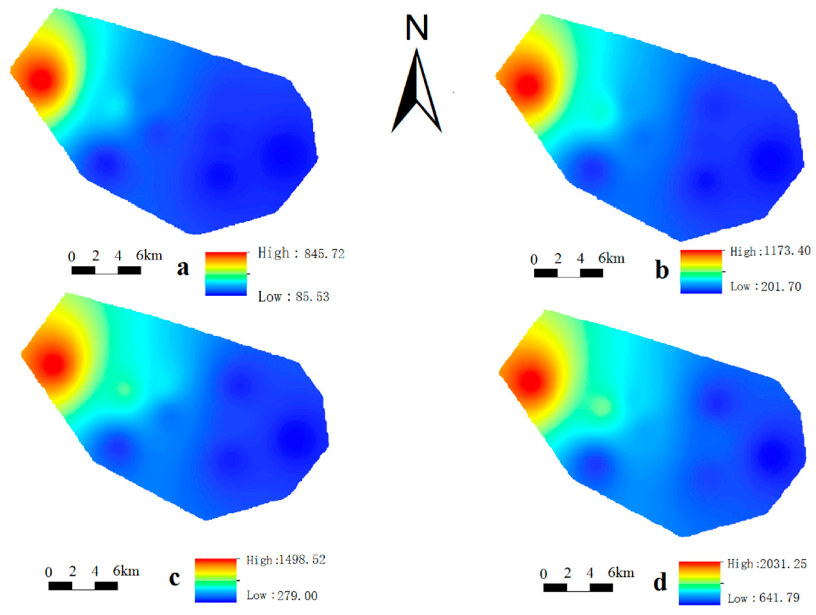
Groundwater depth/level records for 2002–2014 were collected from ten wells. The data were used to analyze the inter-annual spatial variations in groundwater conditions (Figure 3). Generally, there was a clear distinction between the northwest of the Seven Stars–Baoerhai water source reservoir, which showed a higher groundwater depth than the southeast, and the depletion was observed to be seriously spotted in the north. It should also be noted that the central part of the study area showed a lower piezometric groundwater level. The original data analysis has been discussed in Section 3.2 (see Table 4). These findings might suggest that the central part of the basin has been experiencing more water consumption. It could also be deduced that the groundwater depletion has been getting worse from 2002 to 2014. Bosten Lake is located in the eastern of the Seven Stars–Baoerhai water source reservoir, these differences between the variation of the geomorphological characteristics and the piezometric groundwater levels indicate that local surface water played a positive influence on the piezometric groundwater level. Figure 3 shows that groundwater depletion was detected in the water source reservoir, and all of these fluctuations showed a similar downward trend.
3.2. Seasonal Component Analysis
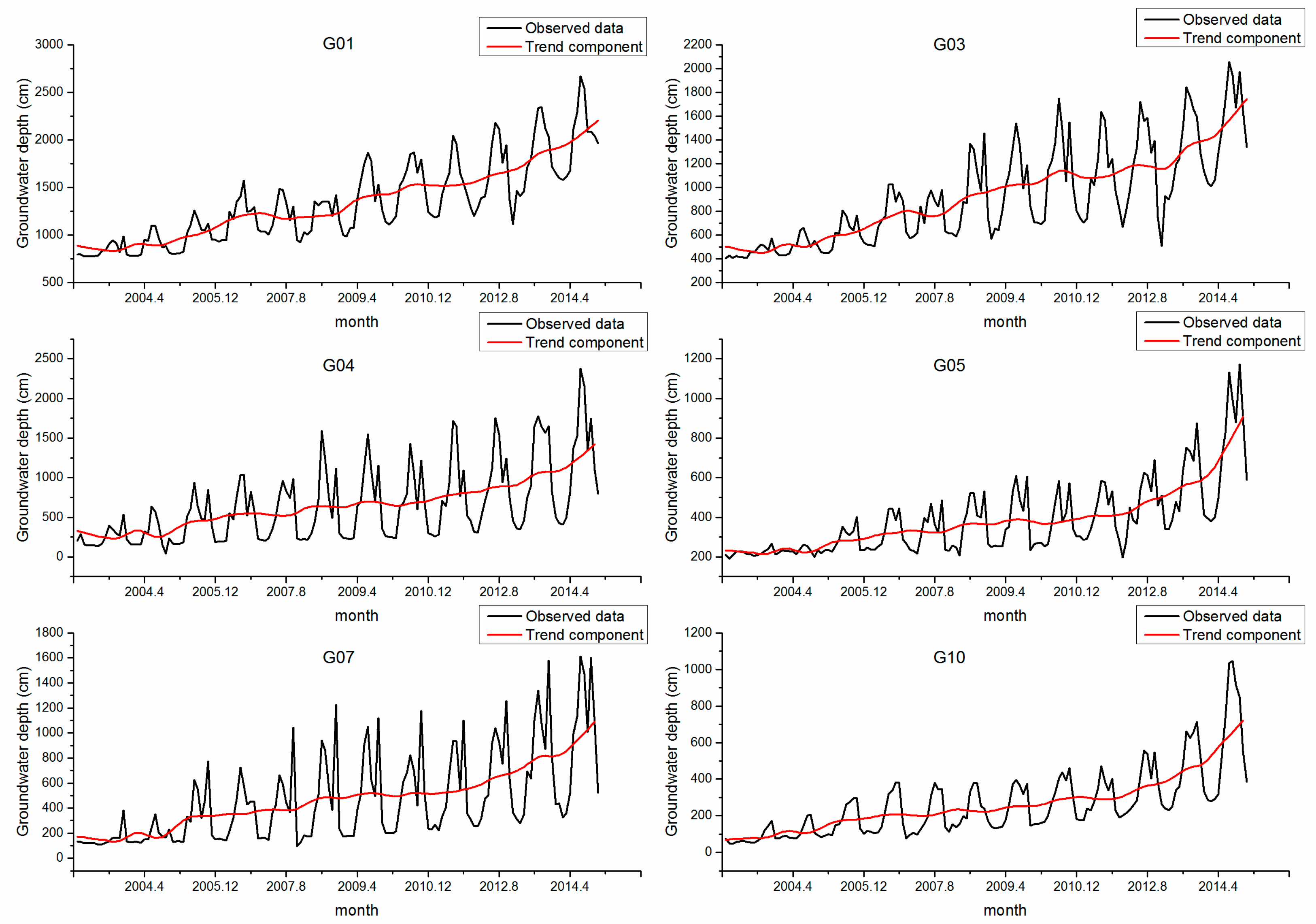
Owning to the fact that the data of the six groundwater sites (G01, G03, G04, G05, G07, and G10) were over the 148 months (from September 2002 to December 2014), while the other four sites were not a complete time-series (Table 1), only these six groundwater sites were detailed analyzed. The STL method was used to investigate the fluctuation characteristics. The groundwater monthly fluctuations and the trend component, which was obtained from the STL decomposition results, have been plotted in Figure 4. As shown in Figure 4, the STL fitted trend was observed in the decomposition plot, in comparison with the raw data. It showed an overall increasing trend in the groundwater depth from 2002 to 2014. As present in Figure 4, the trend component showed minor fluctuations during 2002–2012, while it showed a relatively rapidly rising model, in the year ranging from 2012 to 2014. It also showed a variation and obvious seasonality, across years, for most months. This inter-annual variation was more obvious in the seasonal cycle subseries plot, where particularly, July was the highest point, although a small peak in October was also noted. The seasonal signal detected by STL, agreed with the results of the following Figure 5.
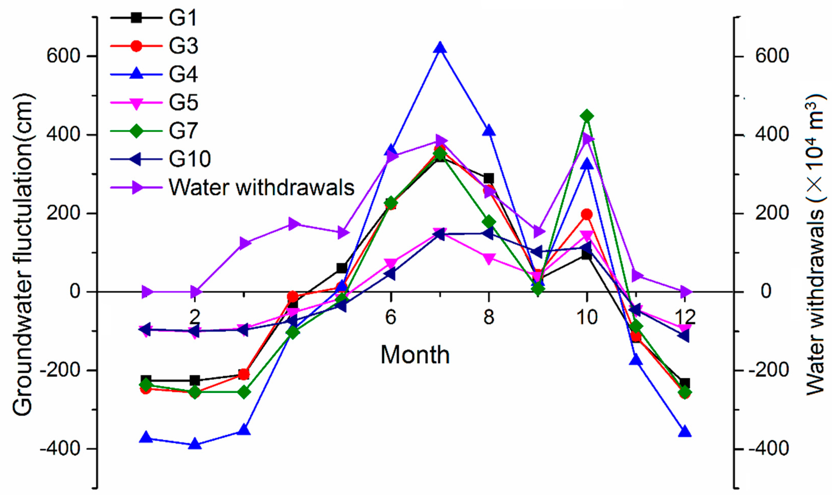
The STL seasonal component and monthly average groundwater exploitation observed (from January 2004 to December 2007) in the decomposition plot (Figure 5). The seasonal patterns suggested an increasing trend in the groundwater depth, from March to November, and a maximal decrease in February. The water withdrawals picture showed that the groundwater mining periods were from March to November, each year, and the groundwater quantity extraction was relatively greater in June, July, and October, respectively. The annual cycle could be divided into two “seasons”, based on the month-to-month variability. The period of “Winter” was approximately November to March and was characterized by a low variability. “Summer” had a much higher variability and lasted from April to October. Figure 5 shows the monthly seasonal component pattern for the groundwater observations. G1, with a peak in July, had a large difference (576.70 cm), with the trough month in December. G3, with a peak in July, had a large difference (620.32 cm), with the trough month in December. G4, with a peak in July, had a tremendous difference (1008.84 cm), with the trough month in February. G5, with a peak in July, had a difference of 253.32 cm, with the trough month in February. G7, with a peak in October, had a large difference (703.62 cm), with the trough month in February. G10, with a peak in August, had a difference of 260.97 cm, with the trough month in December. The seasonal data variation presents a shift in the peak months from July to October, except for September, and the trough months ranged from December to February (Table 3). It was also clear, as shown in Figure 5, that all sites were characterized by a strong seasonal oscillation (for G4, the approximate maximum was 618.833 cm and the minimum was −390.00 cm). This pattern in groundwater change was consistent, across years and across the different sites.
As shown in Figure 5, the monthly seasonal component pattern in September was almost zero, thus, the piezometric groundwater level of September was selected for data analysis (Table 4), and the result could be explained by seasonality. Table 4 summarizes the long-term time trends and seasonal characteristics for all observed wells. Piezometric groundwater level showed a significant decline from 226.90 cm (average value) in September 2002, to 961.50 cm (average value) in September 2014 (Table 4), with an approximate average annual decline of 73.96 cm/year. Likewise, the monthly piezometric groundwater level of all sites showed a downward trend component, with a mean monthly decline of 9.29 cm (G1), 8.78 cm (G3), 8.33 cm (G4), 4.91 cm (G5), 6.67 cm (G7), and 4.54 cm (G10) (Table 3). The average values in Table 4 shows that the depth of the piezometric groundwater level increased rapidly from September 2010 to September 2014; these results could also be validated by Figure 4.
3.3. Monthly Evaluation for Different Sites
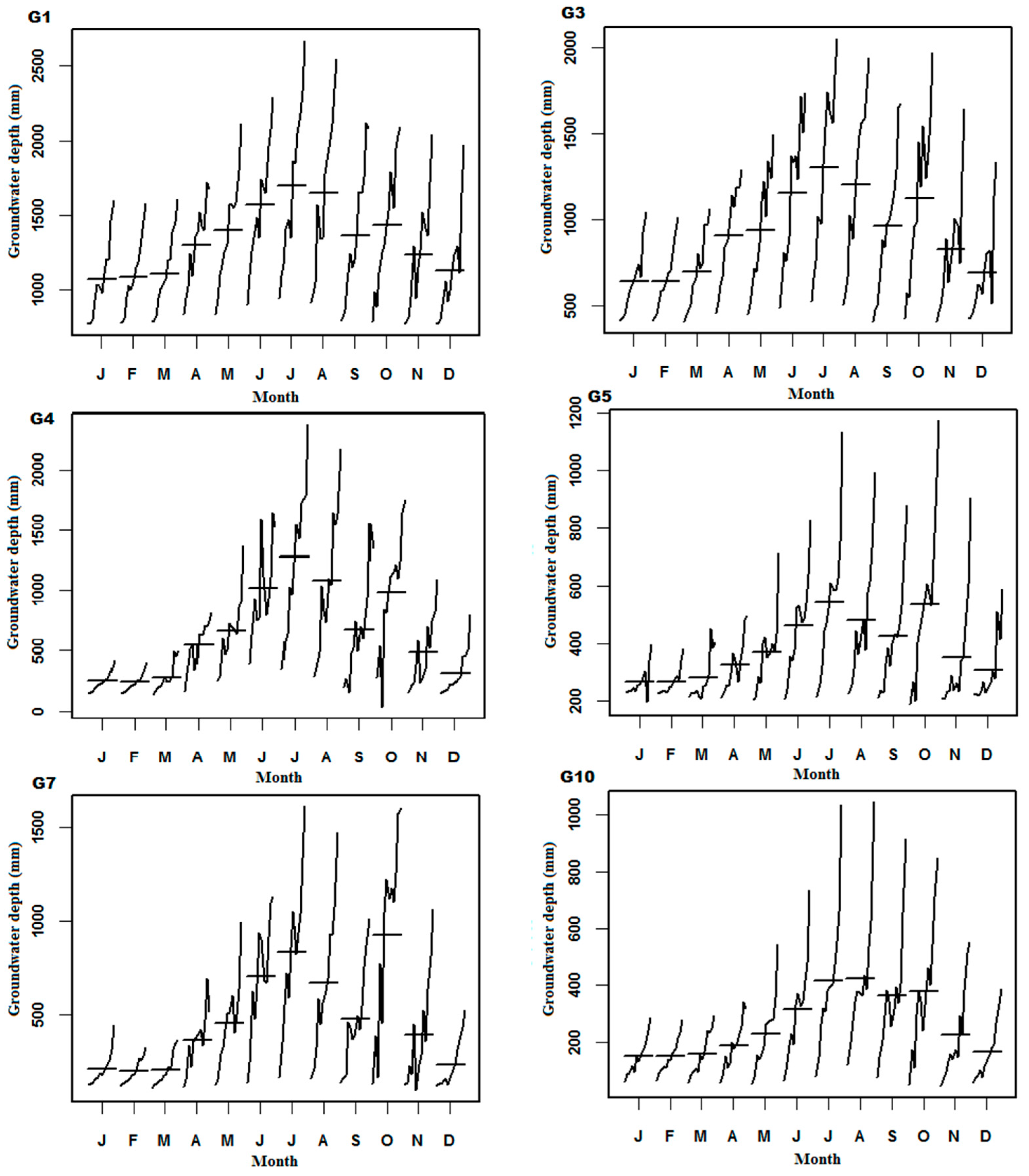
Results regarding the monthly pattern trends over the study period are shown in Figure 6, which showed different monthly series, with different trends. In G1, G3, and G4 site, the seasonal cycle subseries of the monthly plot showed that the average depth of the piezometric groundwater level was highest in July, followed closely by August (Figure 6); the least point emerged in January, and gradual increases occurred with time. However, G5 and G10 displayed different trends from the G1, G3, and G4 sites. The maximum of the average depth of the piezometric groundwater level was in July, followed closely by October (Figure 6), and variability of the mean piezometric groundwater level, between months, was lower than the other regions analyzed. As plotted in Figure 6, the seasonal cycle subseries plot of G7 also showed a different tendency with other sites. G7 showed that the maximum was in October, while the second was observed in July. The average depth of the piezometric groundwater level of January and February was nearly equivalent in all sites. The curve growth and oscillation bending trends also showed that G3, G4, and G7 were in an obviously inter-annual variability. G4 demonstrated the strongest oscillating pattern, especially, in April, May, June, September, October, and November, which was in accord with the mining periods (Figure 5). The variables in January, February, March, and December, in G4, G5, G7, and G10 presented minor growth at each year, while this phenomenon seemed to be inconspicuous in G1 and G3. Although variation among the years existed, the maximum was noted to be in an almost similar month (July or October), for different years and different sites.
3.4. Driving Factors Analysis
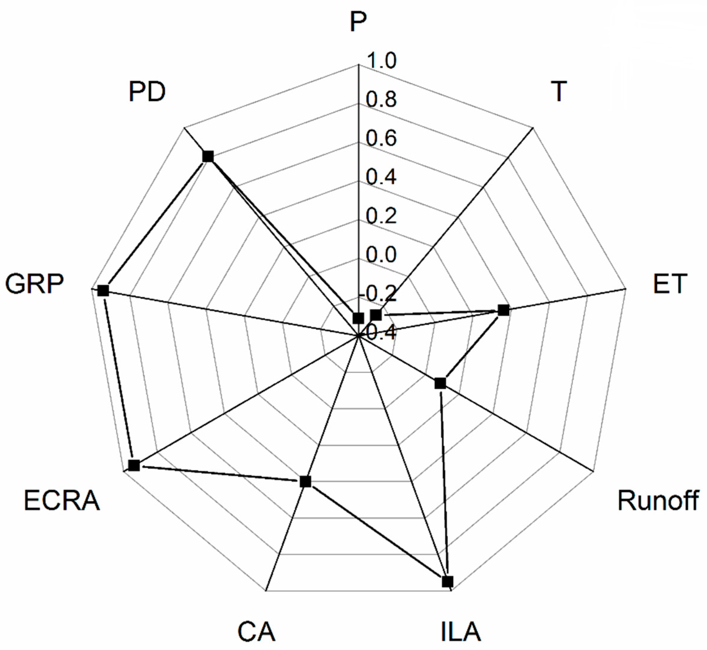
R square is a useful statistical measure to evaluate the regression predictions and is widely used in accuracy measures, for comparisons. Thus, the R square was utilized in this present study. The yearly data ranged from 2003 to 2015 and originated from the Statistical Yearbook of China. Nine factors which were assumed to have a relatively high probability of impact were selected, in terms of two criteria—climate and human activities. These factors were all for statistical dispersion analysis and for the components correlation with groundwater depth. The correlation coefficient variance of each time-series component was calculated (Table 5) and Figure 7 shows the radar plot about the correlation coefficients.
Results showed that, the mean correlation coefficients were 0.95 for the annual irrigated land area, 0.94 for the annual electricity consumed in rural areas, 0.94 for the annual gross regional product, 0.81 for the annual population density, 0.4 for the crop area, 0.36 for the annual mean evapotranspiration, 0.09 for the annual mean runoff, −0.26 for the annual mean temperature, and −0.31 for the annual mean precipitation; the irrigated land area per year was the primary correlation factor (Figure 7). These influenced factors can be classified into two parts—climate change and human activities. The former includes evapotranspiration (ET), temperature (T), runoff and precipitation (P), which were confirmed to have minor or negative correlation effects on the groundwater depth; the latter contained irrigated land area (ILA), electricity consumed in rural areas (ECRA), gross regional product (GRP), population density (PD), and crop area (CA), which were verified to have a high correlation coefficient with a piezometric groundwater level decline, except for crop area.
4. Discussion
Overall, the monthly piezometric groundwater level in the Seven Stars–Baoerhai agricultural irrigation water source in the Tarim basin revealed a consistent downward trend, with a seasonal peak in midsummer and a trough in winter. The present results were highly dependent on the quality and accuracy of the data. Agriculture, especially irrigation, was the principal water user in China, and the Chinese water scarcity condition is deteriorating [8,9,48,49,50]. It is a particular concern to analyze the groundwater depletion in arid land, where agricultural water contributes to most of the domain groundwater decline.
4.1. Trend and Seasonality
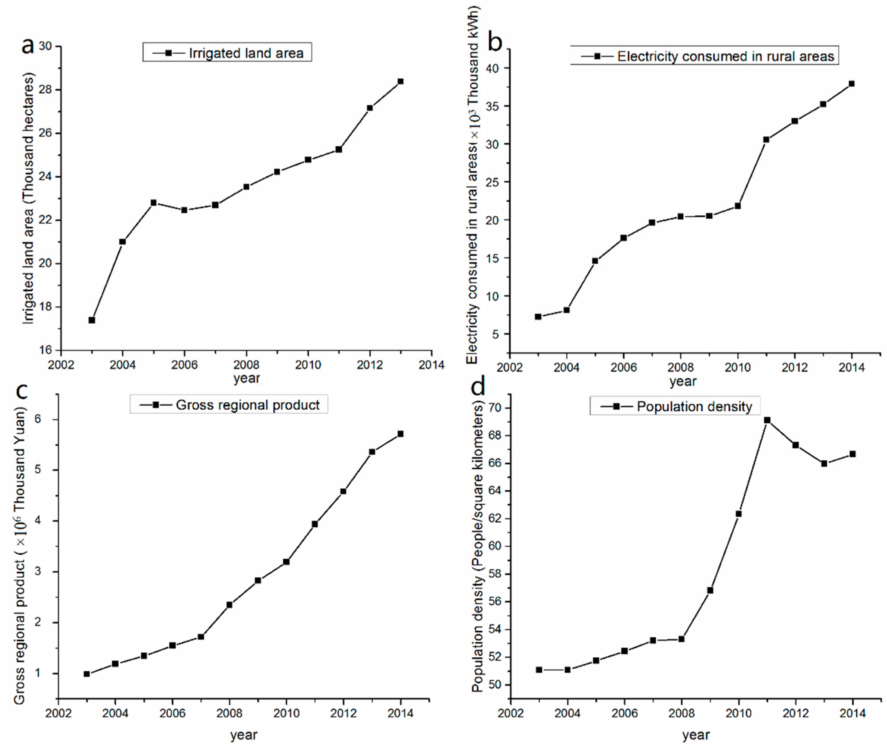
Changes in the month-to-month features were identified using STL, a method that has proven to be highly useful and efficient for analyzing groundwater data covering a time period for more than one annual cycle [36,51]. The trend was summarized with raw data, which showed an overall increasing pattern in groundwater depth from 2002 to 2014 (only minor fluctuations during the year from 2002 to 2012, and a relatively rapidly rising model, from 2012 to 2014). These results might suggest that groundwater extraction volume was on the rise and was strengthened during 2012 to 2014. A correlation analysis was conducted to explore the reason behind groundwater encountering such a rising trend. Yearly change tendencies of the annual ILA (0.95), annual ECRA(0.94), annual GRP(0.94), and annual PD(0.81) has been plotted (Figure 8). Seen from these curves, the ILA presents a sharply increasing trend from 2012 to 2014; the ECRA showed a rapid growth from 2010 to 2014; the GRP also showed a growth from 2007 to 2014; while the annual PD presented a reducing trend during 2011 to 2014. These results might suggest that the irrigated land area could be the major determinant factor, and that other factors could also have a great influence on groundwater depletion.
There is little information on the seasonal-trend decomposition of the intra-monthly variability of groundwater in Tarim River, an arid and semiarid land in China. It was clear that all sites were characterized by obvious variations and had strong seasonal oscillations, across years. The annual cycle was divided into two “seasons” (summer and winter). Most of the seasonal data present a peak month July, and a trough month in December or February. It also identified that the seasonal variability of the “summer” period range was consistent with the exploitation time. A dominant feature found was the seasonal cycle of the mean months. The peak months influenced the model in manner similar to that of groundwater extraction in mining periods (Figure 5). The amplitude of the seasonal signal at those sites, increased after the groundwater was mined and decreased after mining was stopped. These results show that artificial mining has a significant impact on changes in the piezometric groundwater level.
Seasonal cycle subseries plots demonstrated the individual average well piezometric groundwater level, for the same month, in each year. The average depth of the piezometric groundwater level (horizontal line) could be influenced by large values, and these plots were visual representations of the data. Although there were several outliers, almost all monthly curves presented a similar and significant growth trend. These results confirmed that water resource exploitation was continuous in the Tarim Basin and there might have been an over-consumption. The phenomenon that average piezometric groundwater level in January and February seemed to be equal, showed an increasing trend might also provide evidence that water withdrawals play an important role on groundwater decline (Figure 6). The result that G4 presented an obvious inter-annual oscillation bending trend might suggest a possibility that the piezometric groundwater level was more susceptible to artificial exploitation. This is consistent with the earlier finding that the central part might be facing more water consumption. Statistical assessment of factors of groundwater depletion was conducted through a correlation analysis. It was identified that man-made influence factors played a greater role than the natural environmental factors. The variables presented a minor growth in January, February, March, and December in G4, G5, G7, and G10 than other months, in each year, while this phenomenon seemed to be little clear in G1 and G3. It can be explained that the location of G1 and G3 were closer to the desert area (Figure 1) and the groundwater aquifer, in this formation, might be more vulnerable to external environmental impact. Thus, these studies offer evidence that groundwater abstractions exceed the recharge for prolonged periods, and might have a devastating effect on natural ecosystems. It is necessary to formulate some groundwater management measures in water sources to mitigate the trend of groundwater reduction.
4.2. Driving Force Analysis
Overexploitation of water resources might be continuing in the study area. An evaluation was conducted for the correlation between yearly mean piezometric groundwater level and some factors (Table 5). R square was used to evaluate the level of relevance. The impact factors were classified into two patterns (climate change and human activities). It could be identified that human activities played a more important role in the groundwater depletion. A negative relation of precipitation and temperature was observed. It could be deduced that precipitation played a light role on groundwater recharge in the arid land. Snowmelt runoff from the mountains was the main water source for arid land, and the amount of snow melting increased along with temperature increase, which was good for the replenishment of groundwater [52,53]. Combining the research of the STL trend and seasonality, it was held that irrigation could be the primary factor, in accordance with the results of previous research work [8,15,27,54].
It should be also noted that the electricity consumed in rural areas had a significant influence (0.94) on the piezometric groundwater level decline. The result showed that groundwater withdrawals were highly correlated with the electricity consumed in rural areas. In many regions in the Tarim Basin arid land, which covers an area of about 1,020,000 km2, it is a common phenomenon of dig private wells, and these groundwater wells are not equipped with water meters. Electricity can be used to monitor the amount of groundwater quantity when the relationship between electricity and water consumption is determined. The monitoring of electricity is timelier and more accurate than measurement of the irrigated area. Therefore, the monitoring of electricity usage can be more useful to control the exploitation of groundwater, and could also be more accurate and effective than the irrigated area measurement, annual gross regional product, and annual population density.
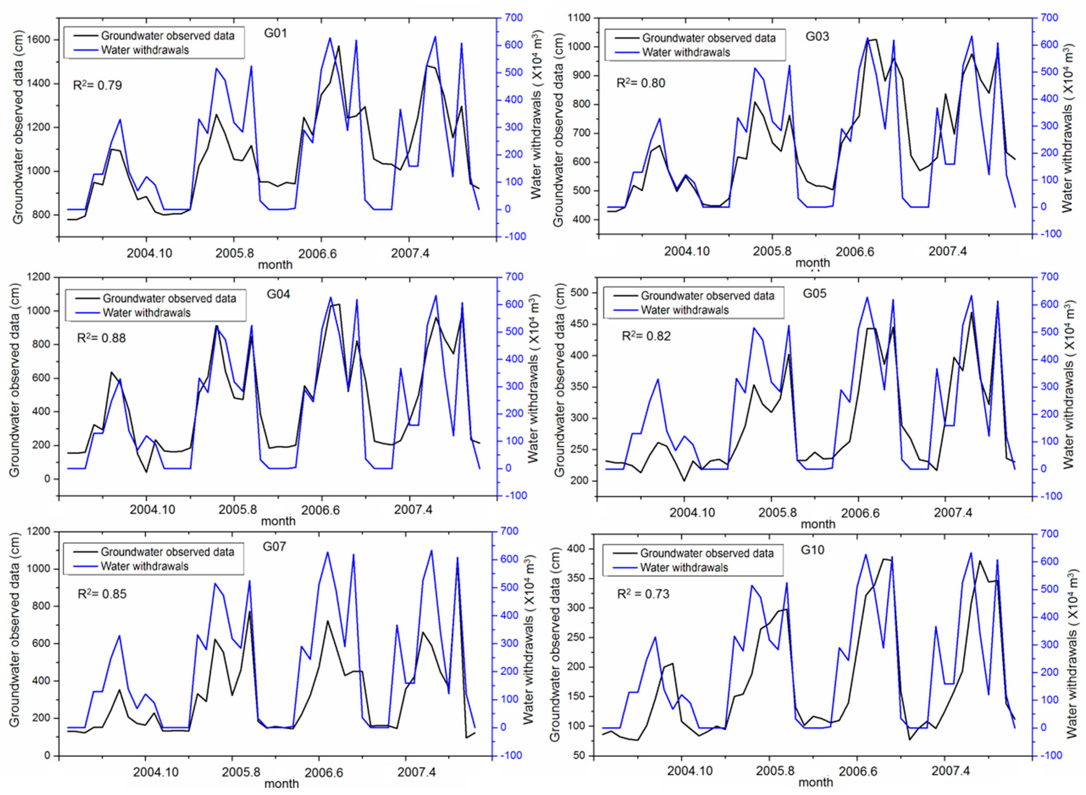
The quantification of groundwater withdrawal might be a hot spot for arid land; this has been studied here. MATLAB’s Curve-Fitting Toolbox with a least squares fitting curve was used for inferring the correlation of groundwater depletion and water withdrawals. Corn, wheat, and cotton were the main crops. The main irrigation technologies included drip tape and flood irrigation [55]. Due to a high correlation between groundwater depletion and water withdrawals, the monthly groundwater withdrawals and groundwater fluctuations data (covered from 2004 to 2007) was fitted to a Linear Fitting curve (R2 = 0.75), along with groundwater level recovery with hysteresis, with a one or two month hysteresis (G1, G3, G4, G5, and G7 was in a one-month hysteresis, and G10 was in a two-month hysteresis, thus, the time lag Δt was one-month in this study, Figure 9).
where Wi−1 is the groundwater withdrawal at the time-step month i − 1, 104 m3; Di is the average groundwater depletion of all these observed wells at the time-step month i (including G1, G3, G4, G5, G7, and G10), in cm; A is the area of agricultural irrigation water resource.
A × Di = 0.66Wi−1 − 612.1
The yearly groundwater withdrawals and groundwater fluctuations data (covered from 2004 to 2007) were also fitted to a Linear Fitting curve (R2 = 0.92):
where Wi is the groundwater withdrawals at the i year, 104 m3; Di is the average groundwater depletion of all these observed wells at the i year (including G1, G3, G4, G5, G7, and G10), in cm; A is the area of the agricultural irrigation water resource. When Di equals 0, the water withdrawal Wi is 860.76 × 10⁴ m3, which shows that it might reach a water balance and the groundwater depth would not increase, to some extent. If the groundwater withdrawals volume was reduced to 860.76 × 10⁴ m3, the associated irrigated areas might have also decreased, and only 70.0% of the current irrigation land area would be used.
A × Di = 0.57Wi − 493.30
4.3. Limitations of the Method
The groundwater change research in a typical arid agricultural irrigate water source, proposed here, has several limitations. For example, it is suitable for a rough estimate of groundwater spatial variation characteristics, since the insufficient underground water wells data and the results might have been affected by the number of observation wells. However, the ten observation wells selected were typical, reasonable, scattered, and the time-series was complete, with sufficient data sequences which could basically represent the groundwater trend of the irrigation water source. The results were influenced by the size of the data, but they could provide a reasonable explanation and evidence.
As groundwater depletion is a complex system process, in this study we have not collected the information on the number of years for which groundwater-discharge/supply took place, which could be modeled by the groundwater numerical model method or traditional water balance method. Both of these methods need a large number of data-points, such as river lateral supply volume, river discharge volume, precipitation infiltration volume, evaporative discharge, and other volumes. The monthly groundwater withdrawals fluctuation might cause the hydrogeological conditions to change monthly (from the river water supply of the irrigated water source to the irrigated water source discharge to the river). In addition, the collected water withdrawal volumes from the irrigated management department and the groundwater withdrawals from common privately dug wells was not included. Thus, there are also many uncertainties in the quantification of groundwater withdrawal.
5. Conclusions
Global groundwater over-exploitation can be seen worldwide, especially in arid and semi-arid lands. Unsustainable water problems have emerged in many countries and are key issues for economic development and food production. The amount of water extracted is higher than water supplied, resulting in decreasing piezometric groundwater level. Water extracted from the earth might temporarily alleviate water shortages.
STL has a clear application in trend and seasonal fluctuation analysis of the piezometric groundwater level and disclosed that artificial mining played a significant role in groundwater depletion. Results obtained from the Seasonal-Trend Decomposition analysis revealed that the trends of piezometric groundwater level in the study’s dryland area continued on a path of significant decline and has become more and more serious, in recent years.
This study also revealed that human activities have strong influence on the groundwater decline, while the effect of climatic changes was insignificant. Results from driving force analysis indicated that irrigation was the primary factor and temperature and precipitation could be used as positive criteria for groundwater recharge. Electricity consumed in rural areas could be an effective, convenient, and practical factor to assess groundwater exploitation in the Tarim Basin. Electricity consumption fluctuations are easier to monitor and calculate than the piezometric groundwater level. The research of the relationship between electricity and water consumption might need further discussion. The optimal groundwater exploitation and irrigation area might be 860.76 × 10⁴ m3 and 70% of the current water withdrawals and irrigation land area, respectively.
Overall, this study indicated that human activities are the main factors affecting the decline of piezometric groundwater level. The problem of groundwater in the agricultural water dryland sources is serious and needs to be highly valued. Groundwater is like a huge reservoir under the earth. It is opaque, concealed, and can be easily ignored; also it is often poorly monitored and not accurately quantified. The relationship between electricity and water consumption may provide a new flexible insight to solve that question. Mechanized production and modern management of farms and irrigation could also be effective for water-saving, and it is also necessary to raise the awareness of farmers regarding water-saving.
Author Contributions
Conceptualization, J.X. and X.W.; methodology, C.Z.; software, Y.Q.; validation, S.H. and P.Y.; investigation, P.Y.; data curation, X.W.; writing—original draft preparation, X.W.; writing—review and editing, L.Z.
Funding
This research was funded by the National Key R&D Program of China (2017YFA0603702), National Natural Science Foundation of China (41890822), and the Project of Climate Change Impacts on Water Resources Management and Adaptation Strategies in Tarim River Basin (TGJJG-2016KYXM0004).
Acknowledgments
The authors also wish to acknowledge the help of Guanghui Wei (Bureau of Xinjiang Tarim River Catchment Administration) for his assistance in the origin data analysis.
Conflicts of Interest
The authors declare no conflict of interest.
References
- Bian, H.; Lu, H.; Sadeghi, A.M.; Zhu, Y.; Yu, Z.; Ouyang, F.; Su, J.; Chen, R. Assessment on the Effect of Climate Change on Streamflow in the Source Region of the Yangtze River, China. Water 2017, 9, 70. [Google Scholar] [CrossRef]
- Yi, S.; Sun, W.; Feng, W.; Chen, J. Anthropogenic and climate-driven water depletion in Asia. Geophys. Res. Lett. 2016, 43, 9061–9069. [Google Scholar] [CrossRef]
- Richey, A.S.; Thomas, B.F.; Lo, M.H.; Famiglietti, J.S.; Swenson, S.; Rodell, M. Uncertainty in global groundwater storage estimates in a Total Groundwater Stress framework. Water Resour. Res. 2015, 51, 5198–5216. [Google Scholar] [CrossRef] [PubMed] [Green Version]
- Famiglietti, J.S.; Lo, M.; Ho, S.L.; Bethune, J.; Anderson, K.J.; Syed, T.H.; Swenson, S.C.; de Linage, C.R.; Rodell, M. Satellites measure recent rates of groundwater depletion in California’s Central Valley. Geophys. Res. Lett. 2011, 38. [Google Scholar] [CrossRef]
- Tague, C.; Grant, G.; Farrell, M.; Choate, J.; Jefferson, A. Deep groundwater mediates streamflow response to climate warming in the Oregon Cascades. Clim. Chang. 2008, 86, 189–210. [Google Scholar] [CrossRef]
- Pokhrel, Y.N.; Koirala, S.; Yeh, P.J.F.; Hanasaki, N.; Longuevergne, L.; Kanae, S.; Oki, T. Incorporation of groundwater pumping in a global Land Surface Model with the representation of human impacts. Water Resour. Res. 2015, 51, 78–96. [Google Scholar] [CrossRef] [Green Version]
- Manga, M. On the timescales characterizing groundwater discharge at springs. J. Hydrol. 1999, 219, 56–69. [Google Scholar] [CrossRef] [Green Version]
- Aeschbach-Hertig, W.; Gleeson, T. Regional strategies for the accelerating global problem of groundwater depletion. Nat. Geosci. 2012, 5, 853–861. [Google Scholar] [CrossRef]
- Wada, Y. Modeling Groundwater Depletion at Regional and Global Scales: Present State and Future Prospects. Surv. Geophys. 2016, 37, 419–451. [Google Scholar] [CrossRef]
- Wada, Y.; van Beek, L.P.H.; van Kempen, C.M.; Reckman, J.W.T.M.; Vasak, S.; Bierkens, M.F.P. Global depletion of groundwater resources. Geophys. Res. Lett. 2010, 37. [Google Scholar] [CrossRef] [Green Version]
- Wada, Y.; van Beek, L.P.H.; Bierkens, M.F.P. Nonsustainable groundwater sustaining irrigation: A global assessment. Water Resour. Res. 2012, 48. [Google Scholar] [CrossRef] [Green Version]
- Siebert, S.; Burke, J.; Faures, J.M.; Frenken, K.; Hoogeveen, J.; Doell, P.; Portmann, F.T. Groundwater use for irrigation—A global inventory. Hydrol. Earth Syst. Sci. 2010, 14, 1863–1880. [Google Scholar] [CrossRef]
- Famiglietti, J.S. The global groundwater crisis. Nat. Clim. Chang. 2014, 4, 945–948. [Google Scholar] [CrossRef]
- Li, X.; Li, G.M.; Zhang, Y. Identifying Major Factors Affecting Groundwater Change in the North China Plain with Grey Relational Analysis. Water 2014, 6, 1581–1600. [Google Scholar] [CrossRef] [Green Version]
- Rodell, M.; Velicogna, I.; Famiglietti, J.S. Satellite-based estimates of groundwater depletion in India. Nature 2009, 460, 999–1002. [Google Scholar] [CrossRef] [PubMed] [Green Version]
- Gleick, P.H. Global freshwater resources: Soft-path solutions for the 21st century. Science 2003, 302, 1524–1528. [Google Scholar] [CrossRef] [PubMed]
- Kummu, M.; de Moel, H.; Porkka, M.; Siebert, S.; Varis, O.; Ward, P.J. Lost food, wasted resources: Global food supply chain losses and their impacts on freshwater, cropland, and fertiliser use. Sci. Total Environ. 2012, 438, 477–489. [Google Scholar] [CrossRef] [Green Version]
- Falkenmark, M. Meeting water requirements of an expanding world population. Philos. Trans. R. Soc. Lond. Ser. B Boil. Sci. 1997, 352, 929–936. [Google Scholar] [CrossRef] [Green Version]
- Alley, W.M.; Leake, S.A. The journey from safe yield to sustainability. Ground Water 2004, 42, 12–16. [Google Scholar] [CrossRef]
- Mays, L.W. Groundwater Resources Sustainability: Past, Present, and Future. Water Resour. Manag. 2013, 27, 4409–4424. [Google Scholar] [CrossRef]
- Steward, D.R.; Bruss, P.J.; Yang, X.; Staggenborg, S.A.; Welch, S.M.; Apley, M.D. Tapping unsustainable groundwater stores for agricultural production in the High Plains Aquifer of Kansas, projections to 2110. Proc. Natl. Acad. Sci. USA 2013, 110, E3477–E3486. [Google Scholar] [CrossRef] [PubMed] [Green Version]
- Zhang, J.; Bai, M.; Zhou, S.; Zhao, M. Agricultural Water Use Sustainability Assessment in the Tarim River Basin under Climatic Risks. Water 2018, 10, 170. [Google Scholar] [CrossRef]
- Chang, B.; Li, R.; Zhu, C.; Liu, K. Quantitative Impacts of Climate Change and Human Activities on Water-Surface Area Variations from the 1990s to 2013 in Honghu Lake, China. Water 2015, 7, 2881–2899. [Google Scholar] [CrossRef] [Green Version]
- Doll, P. Vulnerability to the impact of climate change on renewable groundwater resources: A global-scale assessment. Environ. Res. Lett. 2009, 4, 035006. [Google Scholar] [CrossRef]
- Gleeson, T.; Wada, Y.; Bierkens, M.F.P.; van Beek, L.P.H. Water balance of global aquifers revealed by groundwater footprint. Nature 2012, 488, 197–200. [Google Scholar] [CrossRef]
- Chaudhuri, S.; Ale, S. Long-term (1930–2010) trends in piezometric groundwater levels in Texas: Influences of soils, landcover and water use. Sci. Total Environ. 2014, 490, 379–390. [Google Scholar] [CrossRef] [PubMed]
- Mustafa, S.M.T.; Abdollahi, K.; Verbeiren, B.; Huysmans, M. Identification of the influencing factors on groundwater drought and depletion in north-western Bangladesh. Hydrogeol. J. 2017, 25, 1357–1375. [Google Scholar] [CrossRef]
- Buchanan, S.; Triantafilis, J. Mapping Water Table Depth Using Geophysical and Environmental Variables. Ground Water 2009, 47, 80–96. [Google Scholar] [CrossRef] [Green Version]
- Noori, S.M.S.; Ebrahimi, K.; Liaghat, A.M.; Hoorfar, A.H. Comparison of different geostatistical methods to estimate piezometric groundwater level at different climatic periods. Water Environ. J. 2013, 27, 10–19. [Google Scholar] [CrossRef]
- Varouchakis, E.A.; Hristopulos, D.T. Comparison of stochastic and deterministic methods for mapping piezometric groundwater level spatial variability in sparsely monitored basins. Environ. Monit. Assess. 2013, 185, 1–19. [Google Scholar] [CrossRef]
- Cleveland, R.; Cleveland, W.; Mcrae, J.; Terpenning, I. STL: A seasonal-trend decomposition procedure based on loess. J. Off. Stat. 1990, 6, 3–73. [Google Scholar]
- Hafen, R.P.; Anderson, D.E.; Cleveland, W.S.; Maciejewski, R.; Ebert, D.S.; Abusalah, A.; Yakout, M.; Ouzzani, M.; Grannis, S.J. Syndromic surveillance: STL for modeling, visualizing, and monitoring disease counts. BMC Med. Inform. Decis. Mak. 2009, 9, 21. [Google Scholar] [CrossRef] [PubMed]
- Chaloupka, M. Historical trends, seasonality and spatial synchrony in green sea turtle egg production. Boil. Conserv. 2001, 101, 263–279. [Google Scholar] [CrossRef]
- Bras, A.L.; Gomes, D.; Filipe, P.A.; de Sousa, B.; Nunes, C. Trends, seasonality and forecasts of pulmonary tuberculosis in Portugal. Int. J. Tuberc. Lung Dis. 2014, 18, 1202–1210. [Google Scholar] [CrossRef] [PubMed]
- Isotta, F.; Martius, O.; Sprenger, M.; Schwierz, C. Long-term trends of synoptic-scale breaking Rossby waves in the Northern Hemisphere between 1958 and 2001. Int. J. Clim. 2008, 28, 1551–1562. [Google Scholar] [CrossRef] [Green Version]
- Lafare, A.E.A.; Peach, D.W.; Hughes, A.G. Use of seasonal trend decomposition to understand groundwater behaviour in the Permo-Triassic Sandstone aquifer, Eden Valley, UK. Hydrogeol. J. 2016, 24, 141–158. [Google Scholar] [CrossRef]
- Huang, J.P.; Yu, H.P.; Guan, X.D.; Wang, G.Y.; Guo, R.X. Accelerated dryland expansion under climate change. Nat. Clim. Chang. 2016, 6, 166–171. [Google Scholar] [CrossRef]
- Xia, J.; Ning, L.; Wang, Q.; Chen, J.; Wan, L.; Hong, S. Vulnerability of and risk to water resources in arid and semi-arid regions of West China under a scenario of climate change. Clim. Chang. 2017, 144, 549–563. [Google Scholar] [CrossRef]
- Yang, P.; Xia, J.; Zhan, C.; Qiao, Y.; Wang, Y. Monitoring the spatio-temporal changes of terrestrial water storage using GRACE data in the Tarim River basin between 2002 and 2015. Sci. Total Environ. 2017, 595, 218–228. [Google Scholar] [CrossRef] [PubMed]
- Bureau of Xinjiang Uygur Autonomous Region Water Resources. Xinjiang Water Resources Bulletin. 2015; p. 48. Available online: http://www.xjslt.gov.cn/2017/12/11/slgb/60052.html (accessed on 21 January 2019).
- Guo, M.; Wu, W.; Zhou, X.; Chen, Y.; Li, J. Investigation of the dramatic changes in lake level of the Bosten Lake in northwestern China. Theor. Appl. Climatol. 2015, 119, 341–351. [Google Scholar] [CrossRef]
- Rusuli, Y.; Li, L.; Li, F.; Eziz, M. Water-level regulation for freshwater management of Bosten Lake in Xinjiang, China. Water Sci. Technol. Water Supply 2016, 16, 828–836. [Google Scholar] [CrossRef]
- Xue, L.; Yang, F.; Yang, C.; Chen, X.; Zhang, L.; Chi, Y.; Yang, G. Identification of potential impacts of climate change and anthropogenic activities on streamflow alterations in the Tarim River Basin, China. Sci. Rep. 2017, 7, 8254. [Google Scholar] [CrossRef] [PubMed]
- Hao, X.; Chen, Y.; Xu, C.; Li, W. Impacts of climate change and human activities on the surface runoff in the Tarim River basin over the last fifty years. Water Resour. Manag. 2008, 22, 1159–1171. [Google Scholar] [CrossRef]
- Fan, Y.; Chen, Y.; Liu, Y.; Li, W. Variation of baseflows in the headstreams of the Tarim River Basin during 1960–2007. J. Hydrol. 2013, 487, 98–108. [Google Scholar] [CrossRef]
- Jiang, C.; Zhang, L.; Li, D.; Li, F. Water Discharge and Sediment Load Changes in China: Change Patterns, Causes, and Implications. Water 2015, 7, 5849–5875. [Google Scholar] [CrossRef] [Green Version]
- China Meteorological Administration Meteorological Data Center. Available online: http://data.cma.cn/data/detail/dataCode/ (accessed on 21 January 2019).
- Scanlon, B.R.; Faunt, C.C.; Longuevergne, L.; Reedy, R.C.; Alley, W.M.; McGuire, V.L.; McMahon, P.B. Groundwater depletion and sustainability of irrigation in the US High Plains and Central Valley. Proc. Natl. Acad. Sci. USA 2012, 109, 9320–9325. [Google Scholar] [CrossRef] [Green Version]
- Wada, Y.; Bierkens, M.F.P. Sustainability of global water use: Past reconstruction and future projections. Environ. Res. Lett. 2014, 9, 104003. [Google Scholar] [CrossRef]
- Shamsudduha, M.; Chandler, R.; Taylor, R.; Ahmed, K. Recent trends in piezometric groundwater levels in a highly seasonal hydrological system: The Ganges-Brahmaputra-Meghna Delta. Hydrol. Earth Syst. Sci. 2009, 13, 2373–2385. [Google Scholar] [CrossRef]
- Cristina, S.; Cordeiro, C.; Lavender, S.; Goela, P.C.; Icely, J.; Newton, A. MERIS Phytoplankton Time Series Products from the SW Iberian Peninsula (Sagres) Using Seasonal-Trend Decomposition Based on Loess. Remote Sens. 2016, 8, 449. [Google Scholar] [CrossRef]
- Xu, C.; Chen, Y.; Li, W.; Chen, Y.; Ge, H. Potential impact of climate change on snow cover area in the Tarim River basin. Environ. Geol. 2008, 53, 1465–1474. [Google Scholar] [CrossRef]
- Xu, C.; Chen, Y.; Hamid, Y.; Tashpolat, T.; Chen, Y.; Ge, H.; Li, W. Long-term change of seasonal snow cover and its effects on river runoff in the Tarim River basin, northwestern China. Hydrol. Process. 2009, 23, 2045–2055. [Google Scholar] [CrossRef]
- Lu, Y.; Yan, D.; Qin, T.; Song, Y.; Weng, B.; Yuan, Y.; Dong, G. Assessment of Drought Evolution Characteristics and Drought Coping Ability of Water Conservancy Projects in Huang–Huai–Hai River Basin, China. Water 2016, 8, 378. [Google Scholar] [CrossRef]
- Zhang, P.; Deng, X.; Long, A.; Hai, Y.; Li, Y.; Wang, H.; Xu, H. Impact of Social Factors in Agricultural Production on the Crop Water Footprint in Xinjiang, China. Water 2018, 10, 1145. [Google Scholar] [CrossRef]
Figure 1.
Location of the study area.

Figure 2.
Hydrogeological profile of the study area. The X-axis is the horizontal distant from mountains to the Bosten lake and the Y-axis is the altitude.
Figure 2.
Hydrogeological profile of the study area. The X-axis is the horizontal distant from mountains to the Bosten lake and the Y-axis is the altitude.

Figure 3.
Spatial distribution depths of the piezometric groundwater level (cm) in selected hydrological years: (a) Yearly mean values in 2003; (b) yearly mean values in 2007; (c) yearly mean values in 2010; and (d) yearly mean values in 2014.
Figure 3.
Spatial distribution depths of the piezometric groundwater level (cm) in selected hydrological years: (a) Yearly mean values in 2003; (b) yearly mean values in 2007; (c) yearly mean values in 2010; and (d) yearly mean values in 2014.

Figure 4.
Groundwater monthly fluctuations of observed wells (black line), 2002–2014, and trend component (red line) from the Seasonal-trend decomposition based on the LOESS (STL) decomposition.
Figure 4.
Groundwater monthly fluctuations of observed wells (black line), 2002–2014, and trend component (red line) from the Seasonal-trend decomposition based on the LOESS (STL) decomposition.

Figure 5.
Seasonal subseries plot of the seasonal component estimated by the STL decomposition of depth of the piezometric groundwater level and the annual average groundwater withdrawals.
Figure 5.
Seasonal subseries plot of the seasonal component estimated by the STL decomposition of depth of the piezometric groundwater level and the annual average groundwater withdrawals.

Figure 6.
Seasonal cycle subseries plot of the monthly depth of the piezometric groundwater level in six sites from 2002 to 2014. Horizontal lines display the overall mean value for each month in the thirteen-year period.
Figure 6.
Seasonal cycle subseries plot of the monthly depth of the piezometric groundwater level in six sites from 2002 to 2014. Horizontal lines display the overall mean value for each month in the thirteen-year period.

Figure 7.
Radar plot about the correlation coefficient of the nine factors.

Figure 8.
Yearly change tendency of (a) annual irrigated land area, (b) annual electricity consumed in rural areas, (c) annual gross regional product, and (d) and annual population density.
Figure 8.
Yearly change tendency of (a) annual irrigated land area, (b) annual electricity consumed in rural areas, (c) annual gross regional product, and (d) and annual population density.

Figure 9.
Groundwater (black line) and water withdrawals (blue line) monthly fluctuations of observed wells, 2004–2007.
Figure 9.
Groundwater (black line) and water withdrawals (blue line) monthly fluctuations of observed wells, 2004–2007.


Table 1.
Geographical characteristics of the observation wells and the sampled information.
| Site | Latitude | Longitude | Topographic Ground Altitude (m) | Well Depth (m) | Time Period (Month Year) | Total Epochs (Month) |
|---|---|---|---|---|---|---|
| G01 | 42°03′13″ | 86°19′39″ | 1084.56 | 67.2 | September 2002–December 2014 | 148 |
| G02 | 41°59′44″ | 86°19′13″ | 1064.74 | 67.7 | September 2002–December 2014 | 129 |
| G03 | 42°03′42″ | 86°21′46″ | 1072.82 | 62.2 | September 2002–December 2014 | 148 |
| G04 | 42°01′31″ | 86°22′22″ | 1064.37 | 69.5 | September 2002–December 2014 | 148 |
| G05 | 42°03′25″ | 86°26′29″ | 1061.09 | 65 | September 2002–December 2014 | 148 |
| G06 | 42°01′19″ | 86°26′19″ | 1058.82 | 131.2 | September 2002–December 2014 | 144 |
| G07 | 42°01′13″ | 86°25′52″ | 1059.36 | 67.2 | September 2002–December 2014 | 148 |
| G08 | 41°59′54″ | 86°26′35″ | 1059.48 | 35 | September 2002–December 2014 | 132 |
| G09 | 41°59′04″ | 86°25′59″ | 1057.07 | 72.3 | September 2002–December 2014 | 144 |
| G10 | 42°00′17″ | 86°29′44″ | 1055.78 | 64.4 | September 2002–December 2014 | 148 |
Table 2.
Groundwater withdrawals volume in the Seven Stars–Baoerhai water source from 2004 to 2007.
| Period | Jan. (×104 m3) | Feb. (×104 m3) | Mar. (×104 m3) | Apr. (×104 m3) | May (×104 m3) | Jun. (×104 m3) | Jul. (×104 m3) | Aug. (×104 m3) | Sep. (×104 m3) | Oct. (×104 m3) | Nov. (×104 m3) | Dec. (×104 m3) | Yearly Volume (×104 m3) |
|---|---|---|---|---|---|---|---|---|---|---|---|---|---|
| 2004 | 0 | 0 | 0 | 129.18 | 128.52 | 246.48 | 329.21 | 138.40 | 68.00 | 119.92 | 90.12 | 0 | 1249.83 |
| 2005 | 0 | 0 | 0 | 331.03 | 278.43 | 515.72 | 472.06 | 318.17 | 282.99 | 525.30 | 33.37 | 0 | 2757.07 |
| 2006 | 0 | 0 | 4.67 | 290.23 | 243.74 | 510.74 | 627.56 | 489.58 | 289.65 | 618.89 | 35.05 | 0 | 3110.11 |
| 2007 | 0 | 0 | 366.78 | 158.40 | 158.40 | 524.83 | 633.05 | 342.16 | 120.46 | 608.01 | 118.62 | 0 | 3030.70 |
Table 3.
Groundwater well cases, mean yearly and monthly decline, seasonal peak/trough month and seasonal D-value, 2002–2014.
Table 3.
Groundwater well cases, mean yearly and monthly decline, seasonal peak/trough month and seasonal D-value, 2002–2014.
| Observation Well | Mean Yearly Decline (cm) | Mean Monthly Decline (cm) | Seasonal Peak/Trough Month | Seasonal D-Value a (cm) |
|---|---|---|---|---|
| G01 | 99.12 | 9.29 | July/December | 576.70 |
| G03 | 97.62 | 8.78 | July/December | 620.32 |
| G04 | 88.65 | 8.33 | July/February | 1008.84 |
| G05 | 51.31 | 4.91 | July/February | 253.32 |
| G07 | 67.23 | 6.67 | October/February | 703.62 |
| G10 | 64.65 | 4.54 | August/December | 260.97 |
a D-value was the difference between the value of seasonal peak month and the seasonal trough month.
Table 4.
Linear trend analysis of trend components of the ten groundwater sites recorded during the period 2002 to 2014. The four columns show the monthly change in September, during 2003, 2007, 2010, and 2014.
Table 4.
Linear trend analysis of trend components of the ten groundwater sites recorded during the period 2002 to 2014. The four columns show the monthly change in September, during 2003, 2007, 2010, and 2014.
| Observation Well | September 2003 (cm) | September 2007 (cm) | September 2010 (cm) | September 2014 (cm) | D-Value a (cm) | Annual Change (cm/year) |
|---|---|---|---|---|---|---|
| G01 | 819.67 | 1153 | 1655 | 2081.5 | 1288.5 | 99.12 |
| G02 | 130 | 338 | 484.5 | 939 | 834 | 64.15 |
| G03 | 472.67 | 839 | 1050 | 1673 | 1269 | 97.62 |
| G04 | 269.67 | 744 | 598.5 | 1352.5 | 1152.5 | 88.65 |
| G05 | 239 | 322 | 422 | 879 | 667 | 51.31 |
| G06 | 142 | 352 | 379.5 | 898.5 | 768.5 | 59.12 |
| G07 | 159.67 | 366 | 418 | 1009 | 874 | 67.23 |
| G08 | 150.67 | 402 | 457 | 1035.5 | 910.5 | 70.04 |
| G09 | 120.67 | 317 | 410.5 | 1099 | 1010.5 | 77.73 |
| G10 | 147.33 | 344 | 394 | 917 | 840.5 | 64.65 |
| Average | 226.9 | 517.7 | 626.9 | 1188.4 | 961.5 | 73.96 |
a D-value was the difference between the depth of the piezometric groundwater level at September 2014 and at September 2003.
Table 5.
Correlation coefficient between the nine factors and the depth of the piezometric groundwater level, respectively.
Table 5.
Correlation coefficient between the nine factors and the depth of the piezometric groundwater level, respectively.
| Factors | G1 | G2 | G3 | G4 | G5 | G6 | G7 | G8 | G9 | G10 | Mean | |
|---|---|---|---|---|---|---|---|---|---|---|---|---|
| Sites | ||||||||||||
| P | −0.40 | −0.31 | −0.33 | −0.32 | −0.27 | −0.32 | −0.27 | −0.31 | −0.28 | −0.29 | −0.31 | |
| T | −0.19 | −0.21 | −0.17 | −0.22 | −0.35 | −0.28 | −0.24 | −0.25 | −0.35 | −0.34 | −0.26 | |
| ET | 0.39 | 0.40 | 0.41 | 0.41 | 0.28 | 0.35 | 0.40 | 0.37 | 0.30 | 0.29 | 0.36 | |
| Runoff | 0.15 | 0.12 | 0.12 | 0.13 | 0.06 | 0.08 | 0.03 | 0.09 | 0.06 | 0.09 | 0.09 | |
| ILA | 0.94 | 0.96 | 0.92 | 0.96 | 0.94 | 0.96 | 0.96 | 0.92 | 0.94 | 0.97 | 0.95 | |
| CA | 0.43 | 0.45 | 0.48 | 0.44 | 0.30 | 0.40 | 0.44 | 0.36 | 0.30 | 0.34 | 0.40 | |
| ECRA | 0.96 | 0.95 | 0.94 | 0.96 | 0.90 | 0.94 | 0.94 | 0.95 | 0.92 | 0.91 | 0.94 | |
| GRP | 0.97 | 0.94 | 0.95 | 0.95 | 0.92 | 0.94 | 0.94 | 0.95 | 0.94 | 0.93 | 0.94 | |
| PD | 0.88 | 0.80 | 0.86 | 0.82 | 0.75 | 0.80 | 0.79 | 0.81 | 0.79 | 0.78 | 0.81 | |
© 2019 by the authors. Licensee MDPI, Basel, Switzerland. This article is an open access article distributed under the terms and conditions of the Creative Commons Attribution (CC BY) license (http://creativecommons.org/licenses/by/4.0/).
Share and Cite
MDPI and ACS Style
Xia, J.; Wu, X.; Zhan, C.; Qiao, Y.; Hong, S.; Yang, P.; Zou, L. Evaluating the Dynamics of Groundwater Depletion for an Arid Land in the Tarim Basin, China. Water 2019, 11, 186. https://doi.org/10.3390/w11020186
AMA Style
Xia J, Wu X, Zhan C, Qiao Y, Hong S, Yang P, Zou L. Evaluating the Dynamics of Groundwater Depletion for an Arid Land in the Tarim Basin, China. Water. 2019; 11(2):186. https://doi.org/10.3390/w11020186
Chicago/Turabian StyleXia, Jun, Xia Wu, Chesheng Zhan, Yunfeng Qiao, Si Hong, Peng Yang, and Lei Zou. 2019. "Evaluating the Dynamics of Groundwater Depletion for an Arid Land in the Tarim Basin, China" Water 11, no. 2: 186. https://doi.org/10.3390/w11020186
Note that from the first issue of 2016, this journal uses article numbers instead of page numbers. See further details here.