1. Introduction
Utility companies commonly use closed-circuit television (CCTV) inspections to assess sewer condition. The inspection results can provide support for various levels of decision-making. In the simplest case, they support short-term decisions on whether or not to change a pipe. If the results are further processed and analysed, they can also provide support for mid- and long-term asset management decisions (e.g., [
1,
2,
3]).
Pipe deterioration is known to be a complicated process affected by a multitude of factors [
4]. Although many different factors have been identified as influential or potentially influential (see, e.g., [
4,
5]), it has not been possible to identify a clear set of explanatory variables [
6]. CCTV inspection results have been used both in modelling pipe condition and in analysing influential factors. However, Khan et al. [
7] note that there has been far less focus on assessing explanatory factors as compared to modelling pipe condition or deterioration.
Condition modelling can be carried out at different resolutions, varying from the network level to pipe cohorts and individual pipes. Network level prediction provides support for high-level asset management decisions, for example for estimating the volume of renovation needs and the related budgets. Compared to network level models, pipe cohort models enable improved accuracy in condition estimation and, consequently, better support for e.g., inspection decisions. When the aim is to support decisions on where to target condition inspections, predicting the condition of individual pipes is the best option [
4]. In addition to the spatial resolution, the temporal resolution can also vary from predicting the current condition to predicting the future condition in the mid or long term.
Pinpointing of sewer inspections is a crucial step in sewer asset management, since the inspection results serve as input to renovation decisions and renovation is a costly procedure. Study of how different pipe attributes and environmental variables affect pipe condition provides an understanding of the mechanisms that cause poor condition. This provides valuable information not only for inspection decisions, but also for future installations. This study focuses on modelling the prevailing condition of a pipe network, and hence lifespan models are discussed only when they address factors explaining pipe deterioration.
The methods previously applied for condition modelling include both traditional statistical methods and machine learning methods. Salman and Salem [
8] compared the performance of binary logistic regression, multinomial logistic regression, and ordinal regression in modelling sewer condition. They found ordinal regression to be unsuitable for the study, while binary logistic regression provided the best results. Ariaratnam et al. [
9], Ana et al. [
10], and Fuchs-Hanusch et al. [
11] also applied logistic regression to model poor conditions. Chughtai and Zayed [
12] applied multiple regression to model a five-level sewer condition scale. They created four different models: three for predicting the structural condition of different materials and one for predicting the operational condition. Savic et al. [
13] and Savic et al. [
14] applied a different form of regression, a data-driven modelling algorithm called evolutionary polynomial regression, to model the blockage and collapse events in different pipe classes.
Khan et al. [
7], Tran et al. [
15], and Sousa et al. [
16] applied neural networks to model how different variables affect the condition of the sewer. Tran et al. [
15] modelled the structural condition of stormwater pipes, while Khan et al. [
7] modelled sewer condition and Sousa et al. [
16] the condition of sanitary sewers. Sousa et al. [
16] compared the performance of artificial neural networks (ANNs) and support vector machines (SVMs) with that of logistic regression. They found that ANNs provided the highest classification performance. SVMs, on the other hand, provided excellent results in the study by Mashford et al. [
17], who predicted sewer condition using a five-level scale.
Decision trees were applied by Syachrani et al. [
18] and Harvey and McBean [
19], and random forests by Harvey and McBean [
20]. Syachrani et al. [
18] found that decision trees consistently outperformed the regression and neural networks in predicting the “real age” of sewer pipes. Harvey and McBean [
19] compared the performance of a decision tree with that of SVMs and they found that the decision tree outperformed the SVMs. Harvey and McBean [
20] predicted pipe condition (good/poor) using random forests and obtained good results.
The reported model performance against data varied greatly from one study to another. The multinomial regression in Salman and Salem [
8] correctly predicted the condition rating for 53% of the pipes, while for the SVM model in Mashford et al. [
17] the share was 91%. The rest of the reported fits varied between these two. In spite of the interest in the field, few studies have managed to provide tools for understanding how different predictor variables affect pipe condition. This article studies the use of random forests for predicting an individual pipe’s condition, demonstrates the use of the Boruta algorithm for the analysis of variable importance, and explores partial dependence plots in assessing the effect of different predictor variables on pipe condition.
2. Materials and Methods
2.1. Data Sets and Model Setting
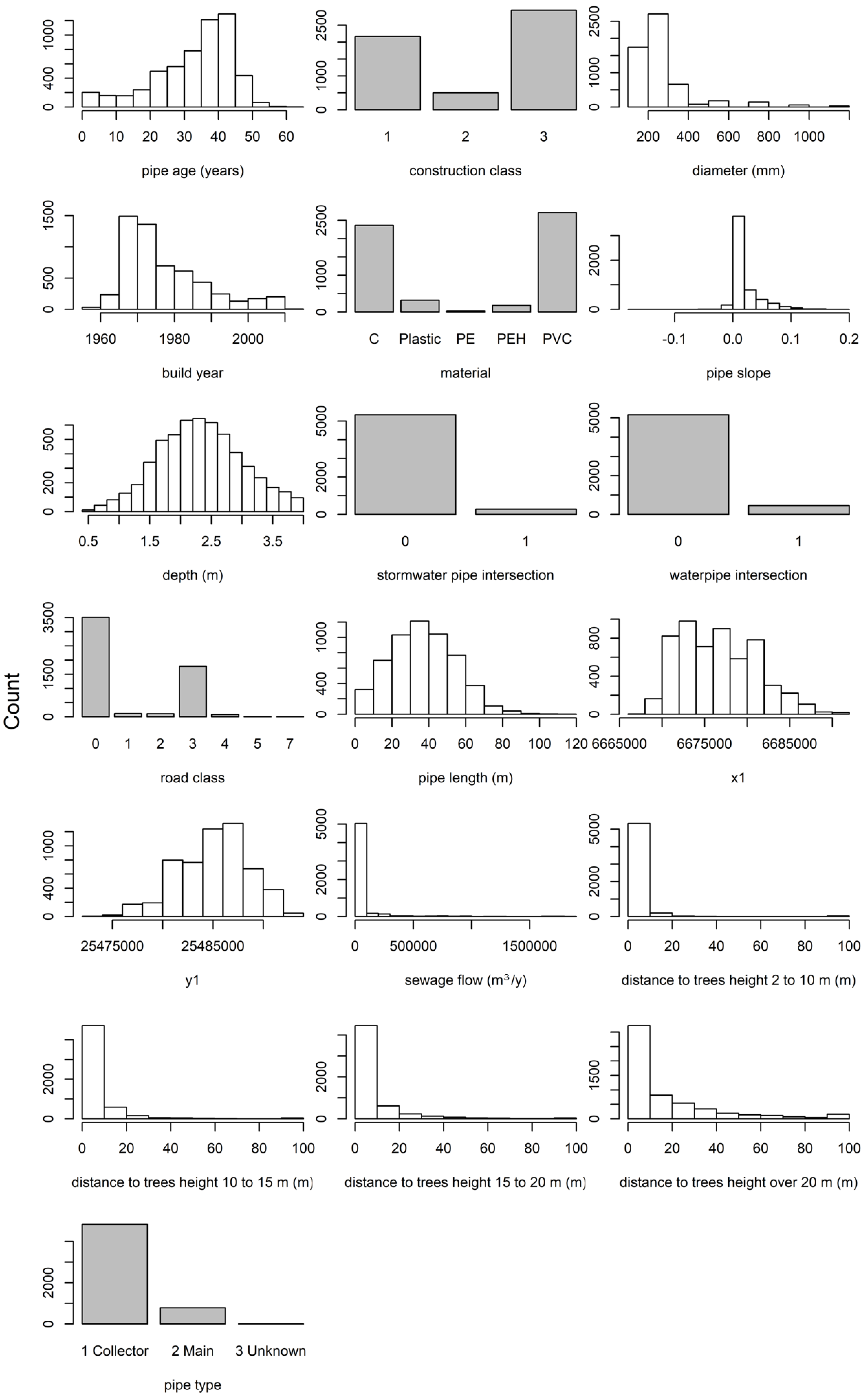
The studied network consists of 1241 km of foul sewers in southern Finland. The network serves a population of approximately 330,000 people and covers an area of ca. 230 km2. The main materials in the network are polyvinyl chloride (47%; PVC), other plastics (29%), and concrete (19%). The share of other miscellaneous materials (iron, glass fibre lining and epoxy lining) is 2% and the material is unknown for 3% of the pipes. The oldest pipes in the network were installed in 1955, and continuous construction has been going on since the 1960s. Approximately 30% of the network was inspected using CCTV between the years 2001 and 2016. So far, the utility company has decided on inspections based on expert judgement. The person carrying out an inspection grades the observations on a five-step scale following the Finnish guidelines for sewer inspections, which are an application of the European standard EN-13508-2 (2003). Score 0 indicates no defect, 1 “slight defect”, 2 “minor defect”, 3 “moderate defect”, and 4 “serious defect”. In the whole data set, 54% of inspected pipes received a score of 2 or lower. The most common defect types in the data set were “deformation”, “root intrusion”, and “surface defect”. These three defect types covered ca. 65% of the total number of defects found.
The complete inspection data set comprises ca. 48,000 observations for ca. 10,000 pipes. In the current analysis, only gravitational pipes and the largest material groups were included.
Figure 1 presents the features of the analysed data set.
As can be seen in
Figure 1, the data set included “concrete”, “PVC”, “PE”, and “PEH”, but also pipes only labelled “plastic”. “Plastic” was the original label and it was kept unchanged. After removing clear outliers, a data set with observations for ca. 6700 pipes remained. Some of these records contained missing attributes, which were estimated using random forest imputation (see
Section 2.3 Random Forest). The data set contained ca. 16,600 maximum score observations, since sometimes there were many observations with the same maximum score for a pipe.
Table 1 presents the 19 studied predictor variables for each pipe, i.e., a network section between subsequent manholes.
The predictor variables included both continuous variables (such as slope) and categorical variables (such as material). The spatial variation of defects was studied using the x- and y-coordinates of the pipe end labelled as number 1 in the utility database. Intersection with water and stormwater pipes was considered, since according to the utility’s experience, defects may appear at pipe intersections. The installation year and age, albeit strongly correlated, are both interesting to study separately, since they reflect different aspects in condition modelling: age represents the impact of pipe age and installation year the impact of, for example, quality of work or material in a given year. For discovering whether the pipe was in poor condition we applied binary classification, where scores 3 and 4 implied “poor” condition and scores lower than 3 implied “acceptable” condition. For each pipe, we selected the maximum defect score from all observations available for that pipe to represent the pipe condition. The aim of the model was to locate pipes with serious defects with the reasoning that these would be in most urgent need of renovation or replacement. Therefore, this model does not consider defects of score 2 or 1 to indicate an inspection need, even if a pipe contains several of these less serious defects.
2.2. Binary Logistic Regression
Binary logistic regression is a statistical method for modelling the connection between a binary outcome (such as existence or absence of poor condition) and predictor variables, which can be numerical or categorical. The binary logistic regression model is formulated as follows [
21]:
where
π(
x) denotes the probability of an outcome
x = (
x1, …,
xp), α is the intercept term, and
β1, …,
βp are regression coefficients for predictor variables
x1, …,
xp. In the binary logistic regression model, the connection between the log odds of an outcome and the predictor variables is linear.
2.3. Random Forest
Random forest is a machine learning method developed by Breiman [
22], and it can be used for classification and regression problems. Machine learning methods can cope with non-linear relationships both between the dependent and the predictor variables as well as between the predictor variables themselves. This is beneficial in the case of sewer condition prediction, since these connections may be non-linear and predictor variables may have interdependencies on many levels. In addition, no pre-categorization is needed.
A random forest is created by generating a multitude (an ensemble) of independent classification trees based on random bagging samples of observations. Additionally, only a subset of variables is selected to form each tree, which adds another layer of randomness to the model creation. The individual trees are weak classifiers and creating an ensemble of trees significantly improves the prediction accuracy compared to creating only one decision tree. Each tree creates a prediction for the class of each observation, i.e., “votes” for a class, and the random forest model chooses the prediction gaining the most votes [
22]. A random forest can operate with data containing numerical and categorical variables and variable values in different scales.
Piragnolo et al. [
23] found indications that random forests perform better than SVMs as training sets get larger. Liu et al. [
24] discovered that random forests clearly outperformed both ANNs and SVMs in an electronic tongue data classification problem. They also state that random forests are able to deal with classification problems of unbalanced, multiclass, and small sample data without data pre-processing procedures.
Random forest imputation is a method for estimating missing variable values. The algorithm starts by a simple replacement of missing values by variable medians for numeric variables and by the most frequent levels for categorical variables. After this, the values are adjusted iteratively. For numeric variables, the estimated values are replaced by the weighted average of the non-missing observations, where the weights are the proximities. For categorical variables, the estimated values become the category with the largest average proximity.
2.4. Adjusting a Binary Model through Changing the Discrimination Threshold
The diagnostic ability of a binary classifier can be assessed using a confusion matrix. A confusion matrix presents predicted and observed labels for all observations as illustrated in
Table 2.
The confusion matrix presents the number of observations in each class. The positive class refers to the existence of an observation such as poor condition and a negative class to its absence. The true positive (TP) cell shows the number of correctly classified positive cases and the true negative (TN) cell the number of correctly classified negative cases. The false negatives (FNs) refer to “missed positive cases” and equal the observations that received a negative label although they are positive. The false positives (FPs), the “false alarms”, refer to those observations classified as positive, although they are negative.
The model accuracy is defined as the fraction of correctly classified observations (Equation (2)).
The true positive rate (
TPR) is the share of positives correctly labelled as positive (Equation (3)) and the true negative rate (
TNR) is the share of negatives correctly labelled as negative (Equation (4)).
Similarly, the false positive rate (FPR) is the share of all negatives incorrectly labelled as positive and the false negative rate (FNR) is the share of positives incorrectly classified as negative. The rates relate to each other through equations FNR + TPR = 1 and FPR + TNR = 1.
When a random forest is applied on a binary classification problem, each tree votes whether or not each observation in the data set belongs to a given class. Typically, the observation is considered to belong to the positive class if the share of positive votes is equal to or higher than 50%, that is, the discrimination threshold is set to 0.5. However, the discrimination threshold can be altered to adjust the diagnostic ability of the classifier. The selection for the optimal threshold depends on the problem context. Often the goal is to maximize the model accuracy, which means maximizing the sum TPR + TNR. Alternatively, the discrimination threshold can also be set to match a desired FNR or FPR.
2.5. Boruta Algorithm and Partial Dependence Plots
Variable selection is the process of finding those predictor variables that are essential for the modelled phenomenon. The Boruta method [
25] is a variable selection algorithm suitable for finding all the variables relevant for the problem. Variable selection is the process of identifying those predictor variables that are essential for explaining the modelled phenomenon. The Boruta method [
25] is a variable selection algorithm for detecting relevant explanatory variables. The algorithm evaluates the effect of each variable on the model result. It finds relevant predictor variables by comparing the original variables’ importance with importance achievable estimated using randomly permuted copies of the predictor variables. It outputs the loss of classification accuracy (a value between 0 and 1) resulting from permutation. In order to get a statistically valid result, the procedure of adding attributes with permuted values and estimating their importance is repeated until the importance is calculated for each of the attributes or, alternatively, the algorithm reaches a predefined number of model runs. The Boruta algorithm is implemented in the R package randomForest [
26].
Friedman [
27] suggested the use of partial dependence plots to visualize and analyse the results produced by a gradient-boosting machine. However, partial dependence plots can be applied to interpret the results produced by any black box learning method [
27]. Partial dependence plots are a means of graphically presenting the relationships between individual predictor variables and a given outcome while the effect of other predictor variables has been averaged out. The partial dependence function is defined as follows [
28]:
In Equation (5), the partial dependence of
f on a subset of variables
Xs is defined as the expectation of
f over the marginal distribution of all variables excluding
s. The subscript
c refers to complementary. The calculation of a partial dependence plot is carried out by averaging over the training data {
Xi,
i = 1, …,
n} with fixed
Xs [
29]:
In a case where a random forest classifier is used to classify observations on a binary scale (such as from poor to good condition) a partial dependence plot depicts the proportion of votes in favour of class 1 (poor condition) against the values of one predictor variable [
28]. The limitation of partial dependence plots is that they can only present the outcome against one or two predictor variables and the low-order interactions between the outcome and the predictors, whereas they are not useful for characterizing or interpreting high-order interactions [
30].
4. Discussion
The created model was able to classify correctly approximately 62% of the previously unseen data, when the
FNR was set to 20%. This is lower than what was hoped for, but in line with the accuracies reported on similar studies. The quality of CCTV inspection data has been found to be deficient in Dirksen et al. [
31], where the authors found that approximately 25% of the defects present on a pipe were missed in an inspection. Even though the rate is likely to be lower for observations in the classes indicating most severe defects, which are the focus of this study, uncertainty in inspection results is a potential reason for decreasing the model accuracy. The reasoning behind why a particular pipe was selected for inspections was not recorded in the database, which causes uncertainty on the results. It would be beneficial to know, for example, whether a pipe was inspected because of a functional problem (e.g., blockage) or because the condition of a network area was assessed for a possible renovation. Boosted regression trees outperformed random forest in predicting water pipe failures in Winkler et al. [
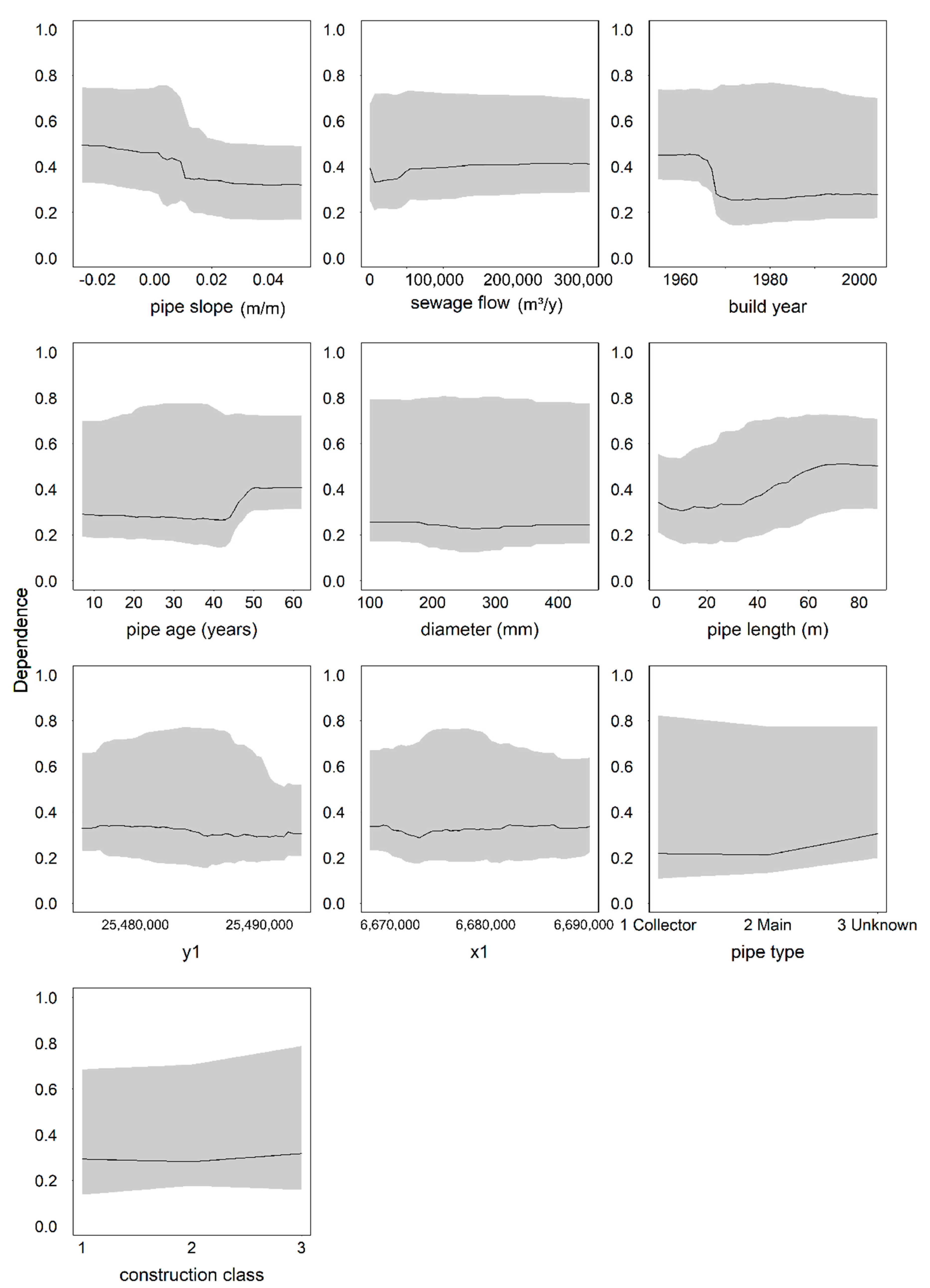
32]. A potential future research topic is to study, whether boosted regression trees or some other modelling method could provide better results than the logistic regression and random forest tested here. The most important predictor variables were identified using the Boruta algorithm and partial dependence plots. In the following paragraphs, we discuss the results on the importance of different variables and compare them to those reported in the literature.
Pipe age has been found influential in various studies (e.g., [
3,
9,
10,
12,
14,
16,
33,
34]). In the network we studied, there was a clear tendency towards poor condition after a pipe age of 44 years. Harvey and McBean [
19] found that the chance of being in poor condition was higher for pipes more than 50 years old, whereas in Egger et al. [
35], the transition to the last condition phase representing the two worst condition classes took place much later: 50% of pipes reached this phase at the age of approximately 65 years.
Fuchs-Hanusch et al. [
11] found that installation year affected pipe condition, whereas in the study by Ana et al. [
10] the construction period had no effect. In our study, the partial dependence of pipe condition on the installation year was clear. Inclusion of both the build year and the pipe age was possible because the selected method allowed high correlation between predictor variables.
In our study, pipes beyond 40 m in length were most likely to have at least one defect indicating poor condition. This was an expected result, since in longer pipes potential length for defects is also higher. Additionally, longer pipes are more prone to bending stresses [
12]. The studied network also has areas where laterals have been connected directly to sewer mains. Direct connections are a potential cause of structural damage and the longer the pipe is, the more connections it may have. Harvey and McBean [
19] found a tendency towards poor condition after a pipe length of 33 m. In contrast, Khan et al. [
7] found that pipes over 70 m in length were in good condition more often than shorter pipes, and the results by Baik et al. [
36] indicated that longer pipes were less likely to deteriorate than shorter ones.
Installation depth was found to be insignificant for pipe condition in the work of Ariaratnam et al. [
9] and Ana et al. [
10], and significant in Sousa et al. [
16] and Caradot et al. [
3]. In the network we analysed, installation depths between 2 m and 3 m were least often connected with poor condition. In contrast, Harvey and McBean [
19] found that the chance of being in poor condition was higher for pipes with an installation depth of 1.9 m or more. As Khan et al. [
7] pointed out, an increase in depth implies greater dead load over the pipe and a higher probability of ground water table affecting the pipe. However, for the network we studied, the minimum recommended installation depth is 1.6 m due to frost in the winter, which could also cause the difference.
Many studies, e.g., [
3,
10,
11,
12,
33,
37,
38] have found that material affects pipe condition, although some studies have suggested the opposite [
9]. Khan et al. [
7] found substantial differences in pipes of different types of concrete, and Syachrani et al. [
18] found essential differences between the deterioration of vitrified clay pipes and PVC pipes. In our data set, only two of the materials, concrete and PEH, appeared as being more often connected with defects than others. This is in line with the work of Sousa et al. [
16], who found differences between only some of the materials they studied. A possible explanation for the slight difference in condition between PEH and other materials is that, according to the utility’s experience, the quality of certain batches of PEH pipes has been deficient. Concrete, on the other hand, has been selected for inspections based on the expert experience that it often may be in bad condition in the analysed network.
Pipe diameter had no effect on pipe condition in the study by Ana et al. [
10]. In many cases, however, diameter has been identified as a significant factor, e.g., [
3,
12,
33,
37]. Khan et al. [
7] found smaller diameters to be more stable as compared to the larger diameters. After 600 mm, there was a subtle tendency towards poor condition. Also, Tscheikner-Gratl et al. [
34] found pipes with higher diameters to deteriorate more slowly. Harvey and McBean [
19] found that the chance of being in poor condition was higher for pipes with a diameter smaller than 238 mm. In our data set, the defects were least common around 1500 mm, and around 300 mm there was a slight tendency towards better condition. According to the utility’s experience, pipes with a diameter around 300 mm are correctly dimensioned considering current wastewater flows. The installation work of large-diameter pipes, on the other hand, is often more carefully supervised than that of other pipes. These reasons could explain their better condition.
Pipe slope was found to be insignificant in the works of Ana et al. [
10] and Caradot et al. [
3], whereas Chughtai and Zayed [
12] and Ahmadi et al. [
33] found a connection between pipe slope and condition. In our study, the connection was clear. Negative and very low slopes were the most harmful ones. Negative slopes and extremely low slopes cause inadequate rinsing, which can lead to debris accumulation and blockages, whereas steep slopes cause high flow velocities which can cause physical erosion in the pipe walls (e.g., [
39]). Our results are in contrast with those by Tscheikner-Gratl et al. [
34], who found pipes with steeper slopes to deteriorate more slowly.
Ana et al. [
10] found location not to affect the pipe condition. In our study, the incorporation of spatial coordinates (
x- and
y-) into the analysis turned out to be useful: spatial variation took place in the occurrence of defects. Two reasons can explain this. First, the network itself exhibits spatial variation, as pipes are not equally spread over the study area. Second, networks are often built subarea-wise and the sub-areas may differ in, for example, quality of installation work, bedding material, land use, and number and type of water consumers served. However, there were pipes in poor condition all over the network, not concentrated only on specific subareas.
Traffic load was found insignificant in Caradot et al. [
3], whereas Chughtai and Zayed [
12] and Ahmadi et al. [
33] found a connection between road class and pipe condition. In our study, the connection with the road class and pipe condition was weak, as was the connection between soil class and pipe condition. Soil type was found to be significant in Micevski et al. [
37] and Savic et al. [
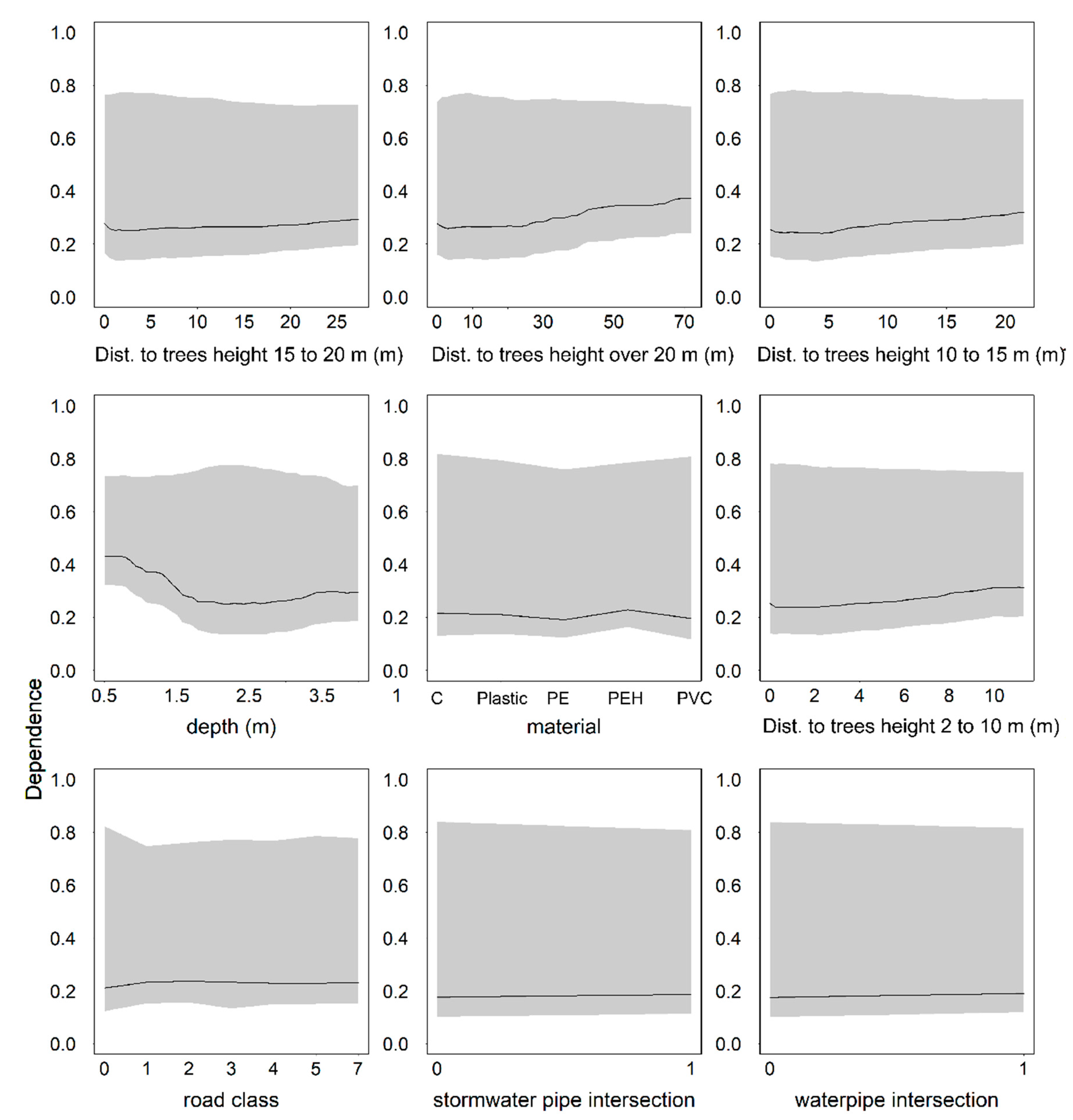
14]. Even though the connection with the soil type was very vague, we must note that a fair number of uncertainties were related to the soil type estimate. Our analysis only covered the soil type at the very location of the observed defect based on soil maps that described the soil type at a 1-m depth (originally extrapolated from point measurements by the data provider). Therefore, more research is needed on the impact of soil type. Although intersection with stormwater pipes and water distribution pipes was originally assumed to affect pipe condition, based on the analysis results, they were insignificant.
We studied the effect of the tree stand using a fairly long maximum distance of 100 m. Most likely this is the reason to the somewhat counterintuitive trend seen in the partial dependence plots, where it seems that pipes are in good condition close to trees. However, when focusing on the distances of 5 m or less, we see that pipes within or close to tree stand are more often in poor condition than pipes farther away. Beyond this distance, there are likely to be many other urban structures between the pipe and tree stand, which complicates the connection. The results suggest that in future research, the distances studied should be limited to a couple of meters from the tree stand.
In our study, pipe and network features were more important than variables related to the soil type or to the vicinity to other infrastructure. The significance of pipe location was thus contradictory: the pipe coordinates were important, but factors related to pipe environment were not significant.
The results we gained on variable importance with the Boruta algorithm were in line with the outcomes provided by the analysis of partial dependencies. However, we denote that while the Boruta algorithm is useful for assessing importance, it provides little support for management decisions, since the structure of the connection between the variables and the condition remains unknown. We also found that even though all of the studied predictor variables were regarded as significant by the Boruta algorithm, a similar predictive power was reached using eight of the most relevant predictor variables.
The analysis on partial dependencies provided insight into the connections between the explanatory variables and poor condition. Since most of the articles reviewed for this study do not illustrate the effect of different predictor variables, a detailed comparison was not possible. Chughtai and Zayed [
12] present the connection between the condition rating and pipe age for some of the predictor variables, considering average values for other variables. Their analysis, however, covers five condition classes, so the results cannot be compared directly with ours. Similarly, Khan et al. [
7] studied the effect of different predictor variables on five condition classes and presented the normalised condition rating as a function of one predictor variable at a time.


