Wave Climate at Shallow Waters along the Abu Dhabi Coast
by
 ,
,
Waleed Hamza
1, 
Letizia Lusito
2,*,
Francesco Ligorio
2,
Giuseppe Roberto Tomasicchio
2 and
Felice D’Alessandro
2 1
Biology Department, College of Science, United Arab Emirates University, 15551 Al Ain, UAE
2
Department of Engineering for Innovation, University of Salento, Campus Ecotekne, 73100 Lecce, Italy
*
Author to whom correspondence should be addressed.
Water 2018, 10(8), 985; https://doi.org/10.3390/w10080985
Submission received: 3 July 2018
/
Revised: 16 July 2018
/
Accepted: 18 July 2018
/
Published: 26 July 2018
(This article belongs to the Special Issue Coastal Vulnerability and Mitigation Strategies: From Monitoring to Applied Research
)
Abstract
:High-resolution, reliable global atmospheric and oceanic numerical models can represent a key factor in designing a coastal intervention. At the present, two main centers have the capabilities to produce them: the National Oceanic and Atmospheric Administration (NOAA) in the U.S.A. and the European Centre for Medium-Range Weather Forecasts (ECMWF). The NOAA and ECMWF wave models are developed, in particular, for different water regions: deep, intermediate, and shallow water regions using different types of spatial and temporal grids. Recently, in the Arabian Gulf (also named Persian Gulf), the Abu Dhabi Municipality (ADM) installed an ADCP (Acoustic Doppler Current Profiler) to observe the atmospheric and oceanographic conditions (water level, significant wave height, peak wave period, water temperature, and wind speed and direction) at 6 m water depth, in the vicinity of the shoreline of the Saadiyat beach. Courtesy of Abu Dhabi Municipality, this observations dataset is available; the recorded data span the period from June 2015 to January 2018 (included), with a time resolution of 10 min and 30 min for the atmospheric and oceanographic variables, respectively. At the ADCP deployment location (ADMins), the wave climate has been determined using wave propagation of the NOAA offshore wave dataset by means of the Simulating WAves Nearshore (SWAN) numerical model, the NOAA and ECMWF wave datasets at the closest grid point in shallow water conditions, and the SPM ’84 hindcasting method with the NOAA wind dataset used as input. It is shown that the best agreement with the observed wave climate is obtained using the SPM ’84 hindcasting method for the shallow water conditions.
1. Introduction
The United Arab Emirates (UAE) is an Arabian Gulf (also named Persian Gulf) nation with an extended coastal area, comprising more than 700 km of coastline and embracing many different shallow water wetland habitats. Some areas of the Abu Dhabi coastline are undergoing a large development with residential, business, cultural, and tourism infrastructure (http://government.ae/en/about-the-uae/uae-future). As a consequence, there is an increasing need for a detailed knowledge of the wave conditions in order to design the coastal interventions [1,2,3,4].
The present study focuses on Saadiyat (Figure 1), a large low-lying 27 km2 island situated in the Gulf within the Emirate of Abu Dhabi. Saadiyat island hosts a vast national park of mangroves and a 9 km SW–NE oriented natural sandy beach, Saadiyat beach, populated by numerous flora and fauna species. Part of the island is undergoing a considerable development program. In March 2015, the “North Beach Phase 1 Development Plans” document was submitted to the Abu Dhabi Urban Planning Council as a part of the Shoreline Protection Works Master Plan, an addendum to the Concept Master Plan of the Saadiyat Cultural District. The urban plan includes the construction of new luxury hotels, a private luxury residential area, and the Cultural District with the Louvre and Guggenheim museums (Figure 2).
At present, professionals involved in the Abu Dhabi coastal development typically use two main sources of wind and wave data: the National Oceanic and Atmospheric Administration (NOAA) and the European Centre for Medium-Range Weather Forecasts (ECMWF), following the well consolidated scientific methods already developed for the analysis of shallow water coastal areas [5,6,7,8,9].
To overcome the scarcity of in situ observations in the area, the Abu Dhabi Municipality (ADM) has recently installed several instruments in the vicinity of the Abu Dhabi coastline at different water depths. Within a research project granted by the National Water Center at the United Arab Emirates University, the new in situ observed wave conditions dataset has been made available.
The in situ observed wave dataset allows for the comparison and verification of data from other sources, such as the NOAA and ECMWF global wave models, third-generation shallow water models such as the Simulating WAves Nearshore (SWAN) [10,11], and second-generation local wave models [12]. The comparison and verification method used is the Shore Protection Manual ’84 (SPM ’84) method [1], a second-generation wave hindcasting method widely used for local hindcasting. SPM ’84 has been selected because of its simplicity in the algorithms and because it allowed for the consideration of different wave regions. SWAN has been already successfully used to model waves in coastal regions [13,14,15,16,17,18,19].
The SPM ’84 method allows the estimation of the wave characteristics using wind data (intensity, direction and duration of the event) at a reference height of 10 m above sea water level, and the effective fetch value. It has been used to calculate the wave conditions at the location where the ADM instrument (ADMins) is deployed from the NOAA wind data, which are provided at 10 m above sea water level.
The comparison and verification of data from NOAA, ECMWF, and SPM ’84 has been conducted under the assumption that the ADMins and the closest NOAA and ECMWF nodes are exposed to homogeneous atmospheric and oceanographic conditions [20,21].
The present paper is organized as follows: Section 2 presents a review of the state-of-the-art of atmospheric and oceanographic global numerical models and the description of the application of the SPM ’84 parametric local wave growth method, Section 3 describes the results, and Section 4 discusses the results from the use of the SPM ’84 wave hindcasting and the adopted verification procedure.
2. Materials and Methods
Recently, the ADM installed an instrument to observe atmospheric (wind speed and direction) and oceanographic (water level, significant wave height, peak wave period, water temperature) characteristics close to the shoreline of the Saadiyat beach. The instrument, an Argonaut-XR produced by the company “SonTek—A Xylem Brand” (San Diego, CA, USA), is a 3-D up-looking monostatic Acoustic Doppler Current Profiler (ADCP) that uses sonar for precise water velocity measurements. Monostatic refers to the fact that the same transducer is used as a transmitter and receiver, with a sampling frequency of 1.5 MHz. Recorded data from June 2015 to January 2018 (included) were available at a time resolution of 10 and 30 min for the atmospheric and oceanographic variables, respectively. The deployed Argonaut-XR presented a limitation: the profiler had not been equipped with the software/hardware necessary to also measure wave spectra; therefore, the instrument could not measure the wave directions directly.
Direct wave measurements are considered the most reliable source of information. In the Gulf area, this type of information is rare or even missing. The Abu Dhabi Municipality started to monitor the wave conditions only four years ago. Other Municipalities in the UAE do not provide directly observed data. As a consequence, at present, the only reliable source of wave data in Abu Dhabi is to consider the new in situ observed wave conditions dataset of sufficient length to represent a mean annual wave climate in relation to the weather conditions in the area, which are quite mild, characterized by the absence of extreme wind conditions (e.g., hurricanes) and extreme wave conditions, due to the fact that the Gulf is an enclosed basin. The wave observations, recorded by the ADCP, have been compared to wave numerical models, designed by some of the major oceanography research centers all over the world.
The first considered model is designed by NOAA. The NOAA National Centers for Environmental Prediction (NCEP) developed the Climate Forecast System (CFS), a fully coupled model representing the interaction between the Earth’s atmosphere, oceans, land, and sea ice. A reanalysis of the sea and atmosphere state for the period of 1979–2009 has been conducted, resulting in the CFS Reanalysis (CFSR) dataset [22]. The purpose of the CFSR is to produce multiyear global, state-of-the-art gridded representations of atmospheric and oceanic states, generated by a consistent model and data assimilation system. The vertical discretization of the atmosphere consists of 64 layers. The temporal resolution for the atmospheric variables is 3 h. Using the CFSR dataset, the NOAA Marine Modeling and Analysis Branch (MMAB) has produced a wave hindcast for the same period. The wave hindcast dataset has been generated using the WAVEWATCH III (WW3) model (v3.14), and it is suitable for use in climate studies. The wave model suite consists of global and regional nested grids. The rectilinear grids were developed using ETOPO-1 bathymetry [23], together with v1.10 of the Global Self-consistent Hierarchical High-resolution Shoreline (GSHHS) database. The higher-resolution North West Indian Ocean bathymetry grid, adopted in the considered data, has a resolution of 10 arc-minutes (1/6°). The WW3 model is run using a 30 arc-minute computational resolution, but the results are interpolated on a 10 arc-minute numerical grid. The spatial resolution of the considered data is, therefore, 1/6°, which corresponds to roughly 20 km. The North West Indian Ocean computational grid, adopted in the considered data, extends in longitude from 30° E to 70° E (with 241 grid nodes) and in latitude from 20° S to 31° N (307 grid nodes). As wave characteristics are dominated by wind dynamics, it is possible to achieve an accurate wave hindcast by using statistically homogeneous wind fields from a long-term reanalysis such as the CFSR, without the need for wave data assimilation [24,25,26]. The NOAA datasets (both wind and waves) are freely available. The NOAA WAVEWATCH III/CFSR webpages [27,28] present additional details about the datasets.
The second of the considered wave hindcasting methods is designed by the European Centre for Medium-Range Weather Forecasts (ECMWF) and it is named ERA-Interim. The ERA-interim dataset is another global atmospheric reanalysis, starting from 1979 and is continuously updated. It is based on the Cy31r2 version of the Integrated Forecasting System (IFS). It also models oceanographic variables, including waves. The atmospheric configuration uses 60 vertical model levels and a 6-hourly temporal resolution [29,30]. The wave model is based on WAM [31,32], resolving 30 wave frequencies and 24 wave directions. The wave model contains corrections for treating unresolved bathymetry effects and a reformulation of the dissipation source term. The bathymetric information is based on the ETOPO-2 bathymetry, with a 2 arc-minute resolution (1/30°). The computational grid resolution for the wave model is 80 km [33], but the output grid has been interpolated onto a finer mesh, of 1/8° horizontal resolution. The ECMWF ERA-Interim dataset is available upon request on the ECMWF servers. Further information on how to access the data can be found at Reference [34].
The SPM ’84 method [1] is a parametric wave hindcasting method; it allows for the determination of the significant wave height (Hs) and peak period (Tp) from (i) the geographical extent of the area where the constant wind is blowing, indicated as fetch (F), (ii) the wind duration (t), and (iii) the depth of water in the generation area (d) [35]. Fetches are related to the curvature of the isobars describing the weather system at the origin of the wave growth. The extent of a typical weather system results in an upper limit for fetches of roughly 500 km.
Given the relative values of F, Tp, and t, the sea state is classified as follows:
- Fully Arisen Sea (FAS), where any added wind energy is balanced by wave energy dissipation and the waves have the maximum possible height;
- Fetch-Limited Sea (FL), where the wave height is limited by the length of the fetch over which the wind has blown; or
- Duration-Limited Sea (DL), where the wave height is limited by the duration of the wind conditions.
The SPM ’84 method determines the spectral significant wave height from , the variance of the sea surface elevation, according to:
where is the zero moment of the wave spectrum, i.e., the area under the spectrum itself. In deep water, is approximately equal to Hs; in shallow water, becomes less than Hs.
The wave growth formulas at both deep and shallow waters are given in terms of the wind stress factor (adjusted windspeed or wind stress), which is related to the normal windspeed at a height of 10 m, , by the following equation:
where both and are measured in m/s. The SPM ’84 method is based on the assumption that the wave growth is entirely caused by a wind blowing at a constant speed and direction for a given duration over the specific fetch area. The wind direction is considered constant if it varies from the wind direction mean by less than 15°, and the wind speed is considered constant if it varies from the wind speed mean by less than 2.5 m/s. With these assumptions and considerations, the equations for wave growth hindcasting/forecasting at shallow water conditions for fully arisen, fetch-limited, and duration-limited sea conditions have been determined. These equations are derived from the analogous deep-water equations [1] with the additional condition that the wave energy is further reduced due to additional effects like bottom friction.
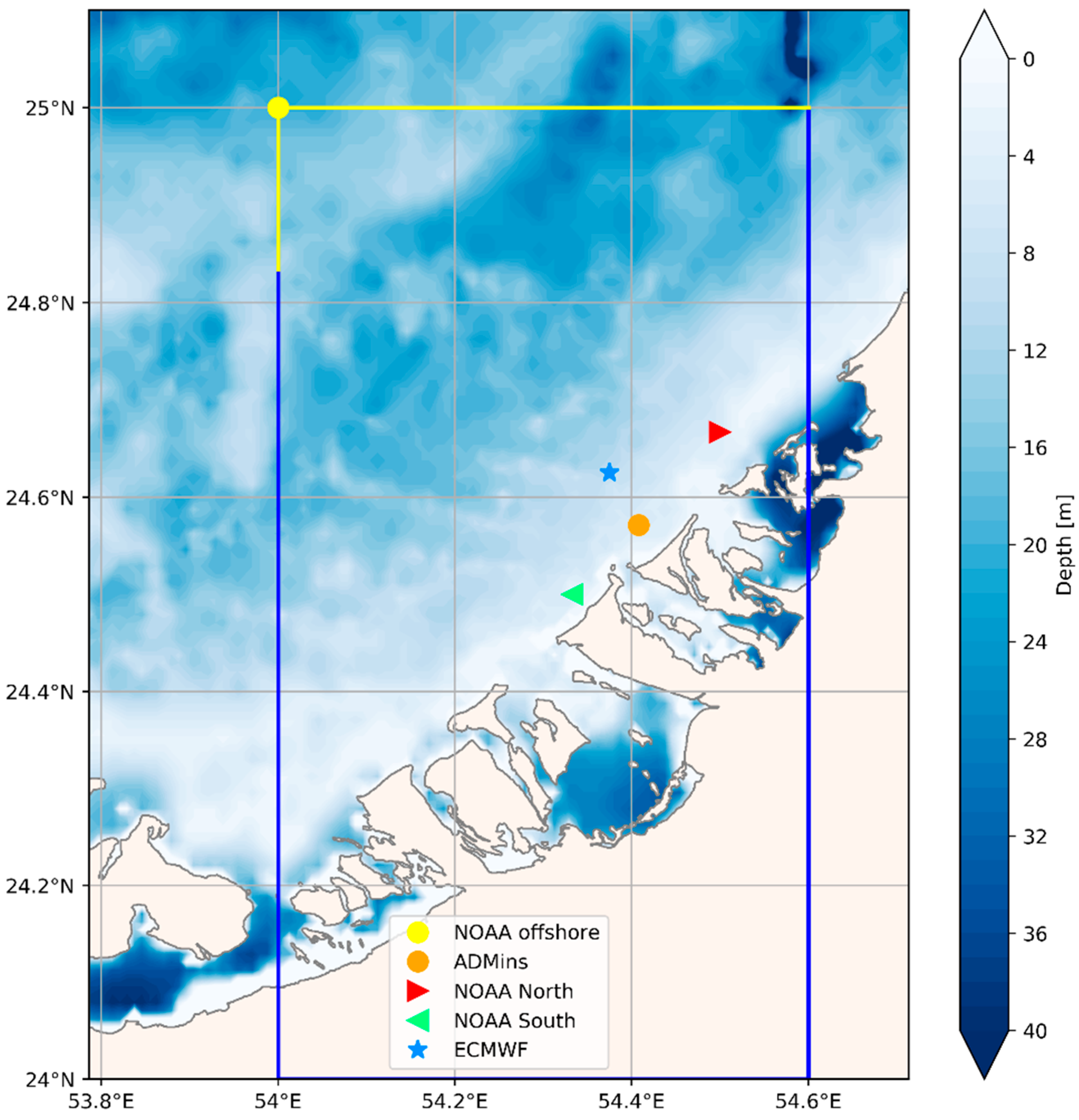
In the present application of wave hindcasting in the Arabian Gulf area, the SPM ’84 input data are the ADMins effective fetches, F [36,37]; the water depth at the ADMins, (equal to 6 m); the wind stress and direction of the wind generating the waves in proximity of ADMins, taken from the NOAA CFSR grid point which is the closest to the ADMins; and the wind duration, t. In the case of Saadiyat beach, there are two NOAA CFSR grid points that are similarly distant from ADMins (Figure 3), located at the north and at the south of the ADMins; in the following, these two grid points will be indicated as NOAA North (NOAA N) and NOAA South (NOAA S). Figure 3 shows the location of the ADMins, the NOAA N and NOAA S grid nodes and the location of the ECMWF grid point. Table 1 reports the coordinates of these grid points, with their corresponding water depths.
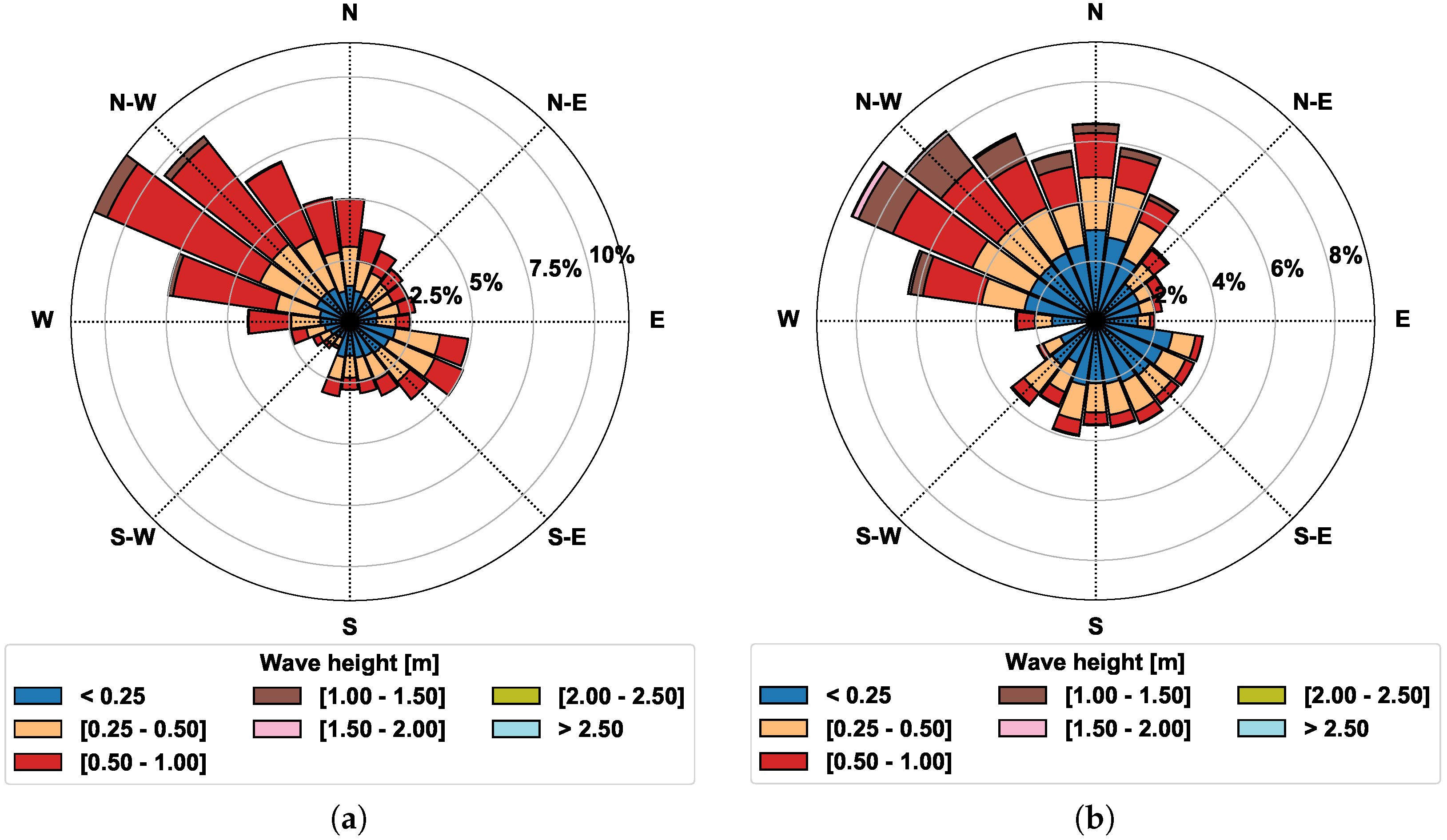
Figure 4 shows the NOAA N (a) and NOAA S (b) wind rose, indicating that the atmospheric conditions at the two locations can be considered uniform. In fact, the NOAA N and NOAA S nodes are exposed to the same atmospheric conditions, given the relatively small distance between the two nodes. Because of this similarity, for the SPM ’84 application, only the data from the north node have been considered; in particular, the wind stress , and wind direction, θ.
The NOAA N wind time series, consisting of approximately 90,000 points, was used to determine an averaged time series of steady wind in both magnitude and direction. A wind measurement datum, i, was considered to belong to a steady weather phenomenon if the following is true:
- | − <>| ≤ 2.5 m/s
- |θi − <θj >| ≤ 15°
where the symbol <> indicated the average of the wind speed calculated over the j points before the ith, already previously “clustered” in a steady wind condition. The same procedure applied for <θj>. If the ith point met the steady state condition, a new average was calculated, aggregating the ith point to the other j. The cluster then contained j + 1 points. Then, the successive point was examined. If a point did not satisfy these conditions, the time-cluster was closed and the location was considered to be subject to a new different wind condition afterwards [38]. The procedure described above is indicated in the following as a “dynamical running average” (DRA). Figure 5 shows the result of the DRA procedure for August 2009. The top panel shows the time series of the wind speed (red) and the dynamically averaged wind speed (blue). The bottom figure shows time series of the wind direction (red) and the dynamically averaged wind direction (blue).
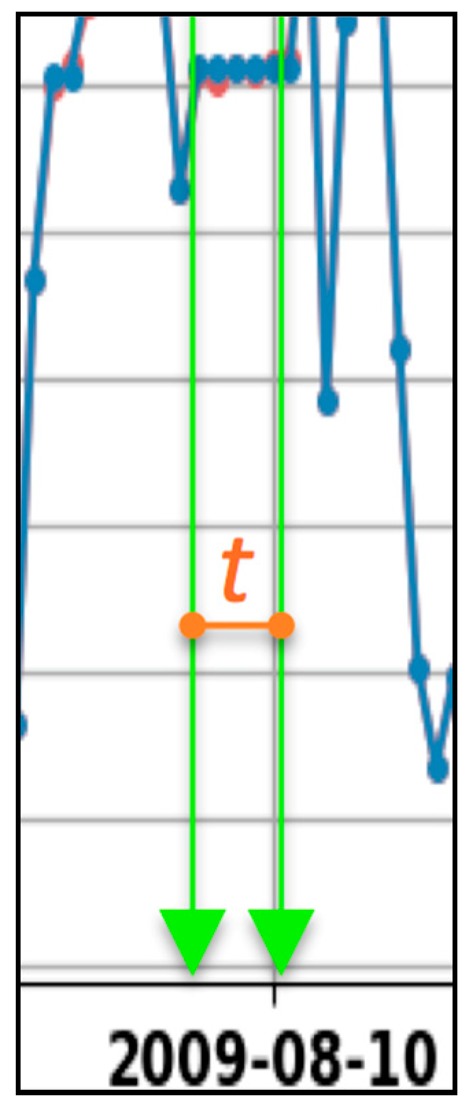
Comparing the DRA wind speed and direction time series (Figure 5, blue lines), only segments where DRA time series are flat in both the wind speed and direction time series were considered (Figure 5, green vertical line). These segments indicated periods of time where the wind conditions were steady (constant). Therefore, the time period between the beginning and the end of these segments has been assumed as the wind duration tADMins of the steady wind phenomenon generating the waves (Figure 6, orange horizontal line). In the example in Figure 6, the resulting duration of the particular wind phenomenon was 15 h (5 data points with 3 h time resolution). If no flat segment could be identified in both the DRA time series, the wind duration was assumed to be 3 h (equal to the time resolution of the original time series).
Having determined the duration of the wind generating the waves, it was possible to apply the SPM ’84 method at the ADMins location, as explained in the following. The wave direction at the ADMins θwave,ADMins was calculated considering the wind–wave direction correlation [39]. Sea regimes (FAS, FL, DL) at the ADMins location, where the water depth was 6 m, were determined as in Reference [40]. If the factor:
FAS exists at the ADMins.
If the ADMins is under the FAS condition, the significant wave height, , was calculated as:
where all the SI units are adopted. If the ADMins was not under the FAS condition, the duration tADMins was compared to the minimum duration, tmin, necessary for establishing the FL condition. The minimum duration was calculated as in Reference [38]:
where is an average water depth along the fetch extension. In this case, . If tADMins < tmin, the location was in the DL condition, otherwise it was in the FL condition.
In the FL condition, the significant wave height at the ADMins, , was calculated as:
In the DL condition, from Equation (5), a new effective fetch was calculated by considering tmin = tADMins and used in Equation (6) to calculate in DL conditions.
Another approach to calculate the wave climate at the ADMins location consisted of propagating the wave dataset at the offshore NOAA grid point towards the coastline. Wave propagation from offshore to ADMins was performed by means of the numerical model SWAN [10,11], which is a third generation fully-spectral wind-wave model developed at the Delft University of Technology (The Netherlands) that simulates random, short-crested wind generated waves in coastal regions.
The offshore wave time series was extracted from the NOAA CFSR model at coordinates 54°00′00″ E, 25°00′00″ N, with water depth equal to 21 m (Figure 3 and Table 1). SWAN was run in stationary mode, in which waves are assumed to propagate instantaneously throughout the model domain. This assumption was reasonable for the small domain and slowly varying forcing conditions for this case. Nonlinear triad interactions [41,42] were significantly larger than quartet interactions for the short spatial scales and shallow depths considered here, and thus quartet interactions were neglected. The model runs included the Madsen expression for bottom friction dissipation [43] using a coefficient of 0.001 m. Breaking wave dissipation was estimated with a bore-based model [44], with the depth-induced constant wave breaking parameter γ = 0.73, found as the mean value of the dataset of Battjes and Stive [45,46]. The frequency, f, and the directional resolution, δ, were defined using the SWAN default values, resulting in 24 logarithmically distributed frequency bins (e.g., Δf ≈ 0.14f [47] over 0.04 ≤ f ≤ 1.00 Hz and 36 10°-wide directional bins Δδ evenly spaced over 0° ≤ δ < 360° [47]). Table 2 summarizes the main SWAN configuration parameters.
The boundary conditions on open boundaries in the north and north-north-west of the computational domain (Figure 3, yellow and blue lines) have been taken from the NOAA WW3 re-analyses, at the coordinates 54°00′00″ E, 25°00′00″ N (Figure 3, yellow dot). Past similar works, e.g., Gorrel et al. [13], suggest that negligible errors in the computing area grids result from the assumption of uniform waves on the N and NNW cross-shore open water boundaries of the grid. The bathymetry information, provided through the “General Bathymetric Chart of the Ocean” (GEBCO) consortium, consists of a gridded terrain model for ocean and land with a spatial resolution of 30 arc-seconds. It was generated by combining quality-controlled ship depth soundings with interpolation between sounding points guided by satellite-derived gravity data [48,49]. Figure 3 shows also the GEBCO bathymetry of the considered area.
Table 3 summarizes the information about the bathymetry and the computational resolution used in SWAN, and in the NOAA and ECMWF wave models.
3. Results
Field measurements showed that the Argonaut-XR appeared to be unable to measure wave peak periods smaller than 3 s, although the instrumental sensitivity range is 2–20 s, according to the system manual technical specifications [52]. Figure 7 shows the wave period normalized probability density function distribution (normalised p.d.f.) as measured by the ADMins, as determined by the NOAA and the ECMWF wave models at the closest location to the ADMins position, and as estimated by the SPM ’84. Figure 7 shows a cut-off at 3 s in the peak period distribution measured by the ADMins. This is not in agreement with the results from the NOAA and ECMWF wave numerical models indicating that waves with a 3 s peak period appear in the area.
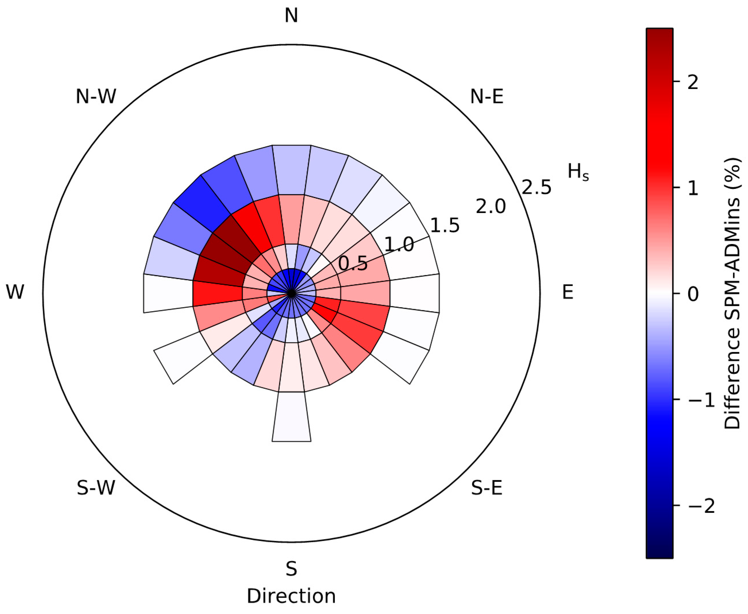
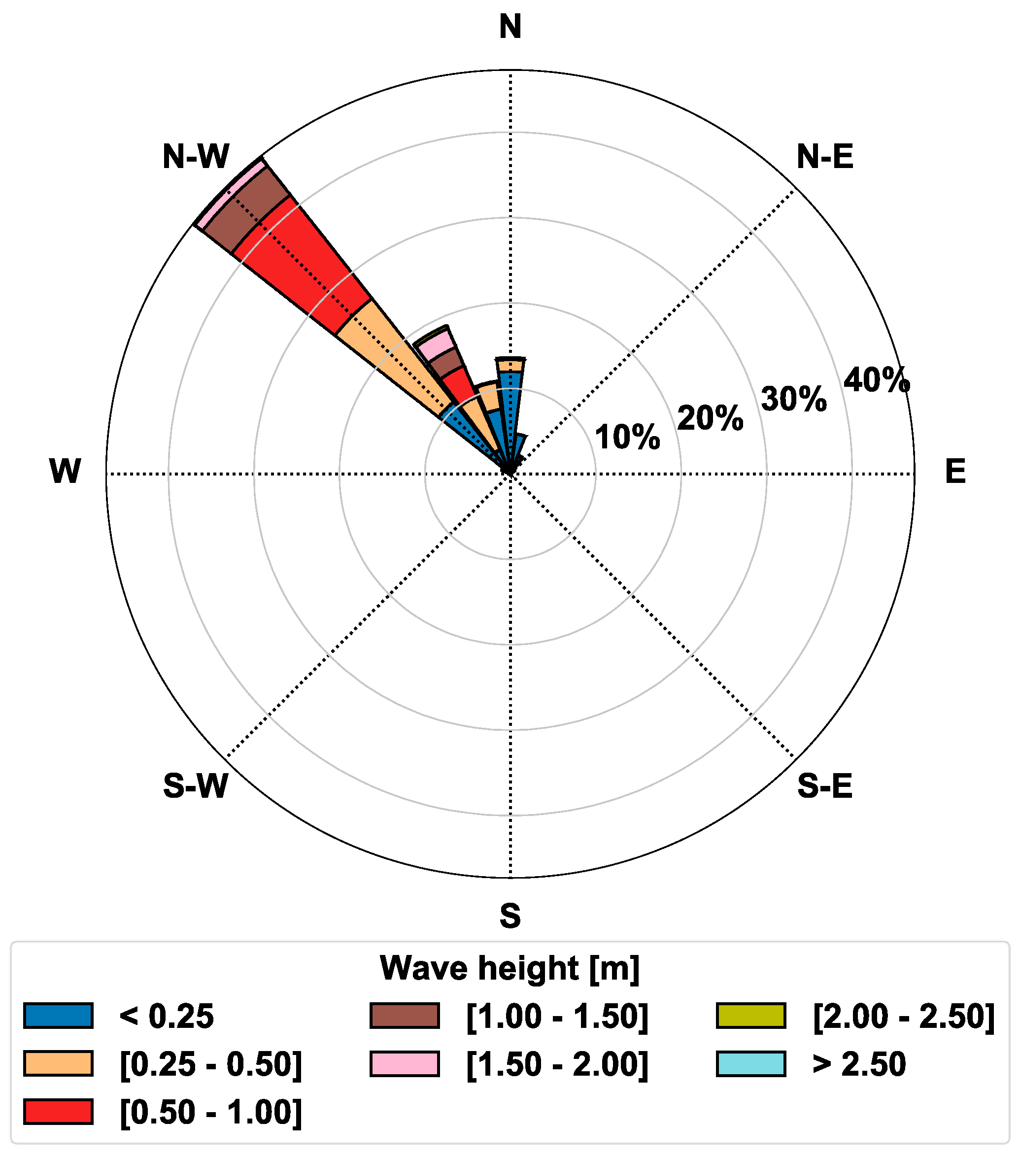
Figure 8 shows the wave roses from SPM ’84 (1979–2009) and ADMins (June 2015–January 2018). The maximum value of the significant wave height, Hs, recorded at a 6 m water depth in front of Saadiyat beach, was around 2 m. The SPM ’84 underestimates the low (0.25–0.50 m) and high (1–2 m) waves, respectively. For each wave height class, Figure 9 depicts the difference between values of appearance frequency (af) in %, determined by SPM ’84 and observed by ADMins; the difference appears to be small, therefore the af determined by SPM ’84 and observed by ADMins are in fairly good agreement. The largest differences were found for values of wave height between 1 and 1.5 m.
Figure 10 shows the wave roses from the NOAA and ECMWF wave models at the nodes, which were closest to ADMins. Comparing the wave roses obtained from the NOAA and ECMWF nodes at shallow water conditions (Figure 10), with the wave roses estimated by SPM ’84 and observed by ADMins (Figure 8) shows that the NOAA and ECMWF models did not sufficiently capture the variability of the wave climate at the ADMins location in shallow water conditions; in particular, for the directional distribution. The higher horizontal resolution (1/8°) of the ERA-Interim wind and waves hindcasted datasets allowed ECMWF to model the waves having Hs between 1.5 and 2 m with better precision compared to NOAA.
Figure 11 shows the SWAN-computed wave rose at the ADMins location. As for the ADMins and SPM ’84, also in this case, the majority of the waves at Saadiyat beach came from the north-west direction, having a wave height of up to 2 m.
Comparing the results from SWAN and SPM ’84 with the observations at the ADMins location, it followed that SWAN was able to reproduce waves with low and high Hs better than the SPM ’84, but the SPM ’84 wave directional distribution presented a better agreement with the observations.
To summarize, Table 4 shows the observed/modelled appearance frequency (af) (in %) in the main sector (NW or numerically 315 ± 22.5°), divided in seven classes of Hs.
With reference to the observations at the ADMins (O), Table 5 shows the af BIAS, af Root Mean Square Error (RMSE), af Normalized BIAS (NBIAS), af Normalized RMSE (NRMSE), Symmetric Mean Absolute Percentage Error (SMAPE), and symmetric RMSE (SRMSE) for the modelled values (M) by: SPM’ 84, SWAN, NOAA N, NOAA S, and ECMWF with respect to the observations, calculated according to:
where the index indicates the Hs class ( = 1, 2,…, 7) and = 7, the number of classes of Hs.
SPM ’84 presented the lowest af RMSE (3.55%), indicating that the standard deviation of the af residuals, i.e., the model error was equal to 3.55% for events in the NW sector. The SWAN af RMSE (8.52%) was lower compared to NOAA N (13.27%) and S (13.20%), and ECMWF (9.36%), confirming the good performance of SWAN under shallow water conditions with respect to the global scale wave models, WAM/WW3, which are more suitable for oceanic large-scale applications.
The main drawbacks of the use of RMSE solely in calculating model performance are the scale dependency (if the model includes variables with different scales or magnitudes, then absolute error measures could not be applied), the high influence of outliers in data on the model performance evaluation, and the low reliability (the results could be different depending on the different fraction of data) [53]. For these reasons, Table 5 shows not only absolute model error statistical indicators, such as BIAS and RMSE, but also indicators based on percentage errors, such as NBIAS and NRMSE. The advantage of such indicators is that they do not depend on the scale of the observations. The disadvantages are that (i) they include a division by 0 if observed data values are very small, (ii) the very high weight of outliers in the final result, (iii) the “asymmetry issue”, and (iv) the error values differ whether the predicted value is bigger or smaller than the actual. For these reasons, a third group of statistical indicators is considered: the so-called “symmetric error” indicators, which are the SMAPE and the SRMSE.
Table 5 shows that the performance of SPM ’84 was the second best considering the SMAPE, after only ECMWF, and followed closely by SWAN. This was due to the fact that both ECMWF and SWAN modelled the contribution of waves with higher Hs better than SPM ’84 in the NW sector, while SPM’84 modelled the directional distribution better.
Analyzing the correlation in each class of Hs between the observations and each model, Figure 12 shows scatter plots of each hindcasting model af versus the observed af. Each subplot shows the values of the coefficient of determination, R2 calculated as:
where SSres is the sum of squares of residuals while SStot is the total sum of squares (proportional to the variance of the data).
The best performance in terms of the correlation was shown by ECMWF (R2 = 0.856) and SWAN (R2 = 0.831); SPM ’84 was third (R2 = 0.618).
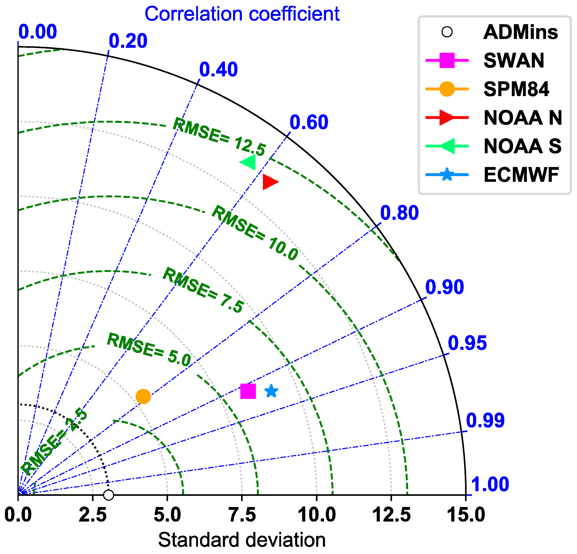
To facilitate the comparative assessment of the different hindcasting models, Figure 13 shows a Taylor diagram [54] representing the performance of each model. Taylor diagrams are used to quantify the degree of correspondence between the modelled and observed behavior in terms of three statistics: the Pearson correlation coefficient, related to the azimuthal angle (in blue), the RMSE (green), and the standard deviation (black). The Pearson correlation coefficient (gauging similarity in pattern between the simulated and observed af) is related to the azimuthal angle; the centered RMSE in the modelled af is proportional to the distance from the point on the x-axis identified as “reference”; and the standard deviation of the modelled af distribution is proportional to the radial distance from the origin. Therefore, Figure 13 shows that all the models had a standard deviation (grey dotted contours) much larger than the observed data, which have a standard deviation of 3.03. The Pearson correlation coefficient was high for SWAN and ECMWF (>90%) compared to SPM ’84 (80%), but SWAN and ECMWF also presented a much higher RMSE (>5%) and a larger standard deviation (>7.5%) compared to the SPM ’84. Therefore, the Taylor diagram showed that the SPM ’84 exhibited the best performance among the considered models.
4. Discussion and Conclusions
Where the ADCP instrument was deployed, the observed wave climate had been obtained and compared with the wave climate determined by means of different models at the same location: wave propagation of the NOAA offshore wave dataset conducted by the SWAN numerical model, assuming wave conditions at the NOAA offshore grid point as boundary conditions; the NOAA and ECMWF wave dataset at the closest grid point; and the SPM ’84 [1] hindcasting method with the closest NOAA wind dataset used as input. The analysis of the wave characteristics has been expressed in terms of distributions of individual wave heights and directions.
The predictive capability of the SPM ’84 has been favorably verified against the observed and calculated wave climates. The estimated af RMSE showed that SPM ’84 resulted in a better agreement with the observed data compared to the other investigated models, and SPM ’84 exhibited the smallest af RMSE (3.55%), followed by SWAN (8.52%), ECMWF (9.36%), and NOAA N and S nodes (13.27% and 13.20%, respectively). Considering a symmetric statistical indicator, such as the SMAPE, SPM ’84 showed a comparable performance to ECMWF and SWAN. The reason for this was that ECMWF and SWAN simulated waves well in the NW sector with high Hs. The principal limitation of the latter two models was their limited representation of the wave directional distribution; mainly due to the assumed NOAA offshore directional distribution and to the limited bathymetrical grid, respectively.
Although SWAN, similarly to WW3 and WAM, used by NOAA and ECMWF, respectively, was a third-generation wave model, it showed better performance in determining the wave characteristics at Saadiyat with respect to NOAA and ECMWF models. This was due to the fact that SWAN contains some additional parameterizations primarily for shallow water [46], different numerical techniques, and different formulations for the wind input and the white-capping with respect to WW3. In addition, it used the higher resolution computational grid and bathymetry in the model implementation, as was shown in Table 3.
A Taylor diagram (Figure 13) of the overall performance of each of the considered wave hindcasting methods showed that the best agreement with the observed wave climate in the vicinity of Saadiyat beach at Abu Dhabi was obtained using the SPM ’84 hindcasting method for the shallow water condition. On the contrary, more sophisticated atmosphere–ocean numerical models, such as those used by NOAA and ECMWF, presented some limitation.
The SPM ’84 best performance could also be due to the fact that the SPM ’84 was based on exact equations (cfr. Equations (3)–(6)) and exact input terms, such as fetches, water depths, wind characteristics, and therefore, not influenced by the resolution of the computational grid or the bathymetric information. The SPM ’84 could be improved, aiming at better modelling waves with high Hs by recalculating the numerical factors that appear in Equations (3)–(6), or calibrating the method before the application by using a subset of the wave observations. In the case of Saadiyat beach, it was not possible to perform this calibration for the time being due to the limited statistics of wave observations collected so far.
The reliability in wave modelling from the application of the SPM ’84 can lead to a better planning of the ambitious coastal interventions that are foreseen in the Gulf area in the next future.
Author Contributions
G.R.T. and L.L. collected all the data, conceived and designed the application of the SPM ’84 method; L.L. analyzed the data, and implemented SWAN and the application of the SPM ’84 method; F.L., W.H., and F.D’A. contributed to the discussion regarding the results; G.R.T. and L.L. wrote the paper.
Funding
This work was funded by the United Arab Emirates University research grant, through the National Water Center, Grant # 31R115; “Impact of coastal (long-shore) currents on erosion/deposition and consequent water/sediments quality variations along the coastal area of Abu Dhabi City” and by the Apulia Region (Italy), through the Regional Cluster Projects “Start”, Grant # 0POYPE3 and “Eco-Smart Breakwater”, Grant # S6LU5I7.
Acknowledgments
The authors thank the Abu Dhabi Municipality for providing in situ data relative to wave conditions at Saadiyat beachfront.
Conflicts of Interest
The authors declare no conflict of interest and the funding sponsors had no role in the design of the study; in the collection, analyses, or interpretation of data; in the writing of the manuscript; or in the decision to publish the results.
References
- United States Army, Corps of Engineers; Coastal Engineering Research Center (USACE). Shore Protection Manual; Department of the Army, Waterways Experiment Station, Corps of Engineers, Coastal Engineering Research Center: Washington, DC, USA, 1984. [Google Scholar]
- Goda, Y. Random Seas and Design of Maritime Structures, 3rd ed.; Advanced Series on Ocean Engineering; World Scientific: Singapore, 2010. [Google Scholar]
- Van der Meer, J.W. Rock Slopes and Gravel Beaches under Wave Attack. Ph.D. Thesis, Delft University of Technology, Delft, The Netherlands, 1988. [Google Scholar]
- Tomasicchio, G.R.; D’Alessandro, F. Wave energy transmission through and over low crested breakwaters. J. Coast. Res. 2013, 1, 398–403. [Google Scholar] [CrossRef]
- Cavaleri, L.; Bertotti, L.; Lionello, P. Shallow water application of the third-generation WAM wave model. J. Geophys. Res. 1989, 94, 8111–8124. [Google Scholar] [CrossRef]
- Stopa, J.E.; Ardhuin, F.; Babanin, A.; Zieger, S. Comparison and validation of physical wave parameterizations in spectral wave models. Ocean Model. 2016, 103, 2–17. [Google Scholar] [CrossRef] [Green Version]
- Rakha, K.; Al-Salem, K.; Neelamani, S. Hydrodynamic Atlas for the Arabian Gulf. J. Coast. Res. 2007, 50, 550–554. [Google Scholar]
- Mazaheri, S.; Ghaderi, Z. Shallow Water Wave Characteristics in Persian Gulf. J. Coast. Res. 2011, 64, 572–575. [Google Scholar]
- Anoop, T.R.; Sanil Kumar, V.; Shanas, P.R. Spatial and temporal variation of surface waves in shallow waters along the eastern Arabian Sea. Ocean Eng. 2014, 81, 150–157. [Google Scholar] [CrossRef]
- Booij, N.; Ris, R.C.; Holthuijsen, L.H. A third-generation wave model for coastal regions, Part I, Model description and validation. J. Geophys. Res. 1999, 104, 7649–7666. [Google Scholar] [CrossRef]
- Ris, R.C.; Booij, N.; Holthuijsen, L.H. A third-generation wave model for coastal regions, Part II, Verification. J. Geophys. Res. 1999, 104, 7667–7681. [Google Scholar] [CrossRef]
- Holthuijsen, L.H. Waves in Oceanic and Coastal Waters; Cambridge University Press: Cambridge, MA, USA, 2007; p. 387. ISBN 978-0521860284. [Google Scholar]
- Gorrell, L.; Raubenheimer, B.; Elgar, S.; Guza, R.T. SWAN predictions of waves observed in shallow water onshore of complex bathymetry. Coast. Eng. 2011, 58, 510–516. [Google Scholar] [CrossRef]
- Brown, J.M. A case study of combined wave and water levels under storm conditions using WAM and SWAN in a shallow water application. Ocean Model. 2010, 35, 215–229. [Google Scholar] [CrossRef]
- Dally, W.R. Comparison of a mid-shelf wave hindcast to ADCP-measured directional spectra and their transformation to shallow water. Coast. Eng. 2018, 131, 12–30. [Google Scholar] [CrossRef]
- Muliati, Y.; Lukman Tawekal, R.; Wurjanto, A.; Kelvin, J.; Pranowo, W.S. Application of SWAN model for hindcasting wave height in Jepara coastal waters, North Java, Indonesia. Int. J. GEOMATE 2018, 15, 114–120. [Google Scholar] [CrossRef]
- Xu, F.; Perrie, W.; Solomon, S. Shallow Water Dissipation Processes for Wind Waves off the Mackenzie Delta. Atmos.-Ocean 2013, 51, 296–308. [Google Scholar] [CrossRef] [Green Version]
- Rogers, W.E.; Kaihatu, J.M.; Hsu, L.; Jensen, R.E.; Dykes, J.D.; Todd Holland, K. Forecasting and hindcasting waves with the SWAN model in the Southern California Bight. Coast. Eng. 2007, 54, 1–15. [Google Scholar] [CrossRef] [Green Version]
- Bottema, M.; van Vledder, G.P. A ten-year data set for fetch- and depth-limited wave growth. Coast. Eng. 2009, 56, 703–725. [Google Scholar] [CrossRef]
- Goda, Y. Spread Parameter of Extreme Wave Height Distribution for Performance-Based Design of Maritime Structures. J. Waterw. Port C ASCE 2004, 130. [Google Scholar] [CrossRef]
- Gencarelli, R.; Tomasicchio, G.R.; Veltri, P. Wave height long term predictions based on the use of the spread parameter. In Coastal Engineering Proceedings, Proceedings of the 30th Conference on Coastal Engineerings (ICCE), Dan Diego, CA, USA, 3–8 September 2006; McKee Smith, J., Ed.; World Scientific: Stevens Point, WI, USA, 2007; pp. 701–713. [Google Scholar]
- Saha, S.; Moorthi, S.; Pan, H.L.; Wu, X.; Wang, J.; Nadiga, S.; Tripp, P.; Kistler, R.; Woollen, J.; Behringer, D.; et al. The NCEP Climate Forecast System Reanalysis. Bull. Am. Meteorol. Soc. 2010, 91, 1015–1057. [Google Scholar] [CrossRef]
- Amante, C.; Eakins, B.W. ETOPO1 1 Arc-Minute Global Relief Model: Procedures, Data Sources and Analysis. In NOAA Technical Memorandum NESDIS; NGDC-24; National Geophysical Data Center: Boulder, CO, USA, 2009; p. 19. [Google Scholar]
- Tolman, H.L. Validation of a new global wave forecast system at NCEP. In Ocean Wave Measurements and Analysis; Edge, B.L., Helmsley, J.M., Eds.; ASCE: Reston, VA, USA, 1998; pp. 777–786. [Google Scholar]
- Tolman, H.L. User Manual and System Documentation of WAVEWATCH-III Version 2.22; NOAA/NWS/NCEP/OMB Technical Note; US Department of Commerce: Washington, DC, USA, 2002; Volume 222, p. 133.
- Tolman, H.L. Testing of WAVEWATCH III Version 2.22 in NCEP’s NWW3 Ocean Wave Model Suite; NOAA/NWS/NCEP/OMB Technical Note; US Department of Commerce: Washington, DC, USA, 2002; Volume 214, p. 99.
- WAVEWATCH III 30-Year Hindcast Wave Model Developed by NOAA (Phase 2). Available online: http://polar.ncep.noaa.gov/waves/hindcasts/nopp-phase2.php (accessed on 4 October 2017).
- The Climate Forecast System Reanalysis [1979–2010]. Available online: http://cfs.ncep.noaa.gov/cfsr/ (accessed on 4 October 2018).
- Berrisford, P.; Dee, D.; Poli, P.; Brugge, R.; Fielding, K.; Fuentes, M.; Kållberg, P.; Kobayashi, S.; Uppala, S.; Simmons, A. The ERA-Interim Archive Version 2.0; ERA Report Series; ECMWF: Shinfield Park, UK, 2011; Volume 1. [Google Scholar]
- Dee, D.P.; Uppala, S.M.; Simmons, A.J.; Berrisford, P.; Poli, P.; Kobayashi, S.; Andrae, U.; Balmaseda, M.A.; Balsamo, G.; Bauer, D.P.; et al. The ERA-Interim reanalysis: Configuration and performance of the data assimilation system. Q. J. R. Meteorol. Soc. 2011, 137, 553–597. [Google Scholar] [CrossRef]
- WAMDI Group. The WAM Model—A Third Generation Ocean Wave Prediction Model. J. Phys. Oceanogr. 1988, 18, 1775–1810. [Google Scholar] [CrossRef]
- Komen, G.J.; Cavaleri, L.; Donelan, M.; Hasselmann, K.; Hasselmann, S.; Janssen, P.A.E.M. Dynamics and Modelling of Ocean Waves; Cambridge University Press: Cambridge, MA, USA, 1994; p. 532. [Google Scholar]
- ECMWF. Part VII: ECMWF Wave Model; ECMWF IFS Documentation—Cy43r3 Operational Implementation 11 July 2017; Technical Report; ECMWF: Reading, UK, 2017. [Google Scholar]
- ERA-Interim. Available online: https://www.ecmwf.int/en/forecasts/datasets/reanalysis-datasets/era-interim (accessed on 10 April 2018).
- Kamphuis, J.W. Introduction to Coastal Engineering and Management; World Scientific: Stevens Point, WI, USA, 2000; p. 437. ISBN 978-981-283-484. [Google Scholar]
- Seymour, R.J. Engineers Estimating Wave Generation on Restricted Fetches. ASCE J. Waterw. Port. C 1977, 103, 251–264. [Google Scholar]
- Smith, J. Wind-Wave Generation on Restricted Fetches; Department of the Army, Waterways Experiment Station, Corps of Engineers, Coastal Engineering Research Center: Washington, DC, USA, 1991. [Google Scholar]
- Karimpour, A.; Chen, Q.; Twilley, R.R. Wind Wave Behavior in Fetch and Depth Limited Estuaries. Sci. Rep. 2017, 7, 40654. [Google Scholar] [CrossRef] [PubMed] [Green Version]
- Leenknecht, D.A.; Szuwalski, A.; Sherlock, A.R. Automated Coastal Engineering System (ACES); Department of the Army, Waterways Experiment Station, Corps of Engineers, Coastal Engineering Research Center: Washington, DC, USA, 1992; p. 373. [Google Scholar]
- Hanley, K.E.; Belcher, S.E.; Sullivan, P.P. A Global Climatology of Wind–Wave Interaction. J. Phys. Oceanogr. 2010, 40, 1263–1282. [Google Scholar] [CrossRef] [Green Version]
- Freilich, M.; Guza, R. Nonlinear effects on shoaling surface gravity waves. Philos. Trans. R. Soc. Lond. A 1984, 311, 1–41. [Google Scholar] [CrossRef]
- Elgar, S.; Guza, R. Observations of bispectra of shoaling surface gravity waves. J. Fluid Mech. 1985, 161, 425–448. [Google Scholar] [CrossRef]
- Madsen, O.S.; Poon, Y.-K.; Graber, H.C. Spectral wave attenuation by bottom friction: Theory. In Proceedings of the 21th International Conference on Coastal Engineering, Costa del Sol-Malaga, Spain, 20–25 June 1988; ASCE: Reston, VA, USA, 1988; pp. 492–504. [Google Scholar]
- Battjes, J.; Janssen, J. Energy loss and set-up due to breaking of random waves. In Proceedings of the 16th International Conference on Coastal Engineering, Hamburg, Germany, 27 August–3 September 1978; pp. 569–587. [Google Scholar]
- Battjes, J.; Stive, M. Calibration and verification of a dissipation model for random breaking waves. J. Geophys. Res. 1985, 90, 9159–9167. [Google Scholar] [CrossRef]
- The SWAN Team. Scientific and Technical Documentation SWAN Cycle III Version 41.20A; Delft University of Technology: Delft, The Netherlands, 2018. [Google Scholar]
- Booij, N.; Haagsma, I.J.; Holthuijsen, L.; Keiftenburg, A.; Ris, R.; van der Westhuysen, A.; Zijlema, M. SWAN Cycle-III Version 40.41 User Manual; Delft University of Technology: Delft, The Netherlands, 2004; 39p. [Google Scholar]
- GEBCO. The GEBCO_2014 Grid, Version 20150318. Available online: www.gebco.net (accessed on 19 July 2018).
- Weatherall, P.; Marks, K.M.; Jakobsson, M.; Schmitt, T.; Tani, S.; Arndt, J.E.; Rovere, M.; Chayes, D.; Ferrini, V.; Wigley, R. A new digital bathymetric model of the world’s oceans. Earth Space Sci. 2015, 2, 331–345. [Google Scholar] [CrossRef]
- Komen, G.J.; Hasselmann, K.; Hasselmann, H. On the Existence of a Fully Developed Wind-Sea Spectrum. J. Phys. Oceanogr. 1984, 14, 1271–1285. [Google Scholar] [CrossRef] [Green Version]
- Hasselmann, K.; Barnett, T.P.; Bouws, E.; Carlson, H.; Cartwright, D.E.; Enke, K.; Ewing, J.A.; Gienapp, H.; Hasselmann, D.E.; Kruseman, P.; et al. Measurements of wind-wave growth and swell decay during the Joint North Sea Wave Project (JONSWAP). Ergnzungsheft zur Deutschen Hydrographischen Zeitschrift Reihe 1973, 8, 95. [Google Scholar]
- Sontek. 2000 SonTek/YSI ADP® Acoustic Doppler Profiler Technical Documentation; SonTek/YSI: San Diego, CA, USA, 2000. [Google Scholar]
- Shcherbakov, M.V.; Brebels, A.; Shcherbakova, N.L.; Tyukov, A.P.; Janovsky, T.A.; Kamaev, V.A. A Survey of Forecast Error Measures. World Appl. Sci. J. 2013, 24, 171–176. [Google Scholar] [CrossRef]
- Taylor, K.E. Summarizing multiple aspects of model performance in a single diagram. J. Geophys. Res. 2001, 106, 7183–7192. [Google Scholar] [CrossRef] [Green Version]
Figure 1.
Aerial view of Saadiyat beach.

Figure 2.
Concept Master Plan of Saadiyat Cultural District (courtesy Tourism Development & Investment Company).
Figure 2.
Concept Master Plan of Saadiyat Cultural District (courtesy Tourism Development & Investment Company).

Figure 3.
Bathymetry of the Saadiyat area, where markers show the position of ADMins, the NOAA N, the NOAA S, the NOAA offshore and the ECMWF model nodes.
Figure 3.
Bathymetry of the Saadiyat area, where markers show the position of ADMins, the NOAA N, the NOAA S, the NOAA offshore and the ECMWF model nodes.

Figure 4.
NOAA wind rose at the north node (a), and at the south node (b), in proximity of the ADMins, indicating that the atmospheric conditions along this stretch of coast can be considered uniform.
Figure 4.
NOAA wind rose at the north node (a), and at the south node (b), in proximity of the ADMins, indicating that the atmospheric conditions along this stretch of coast can be considered uniform.
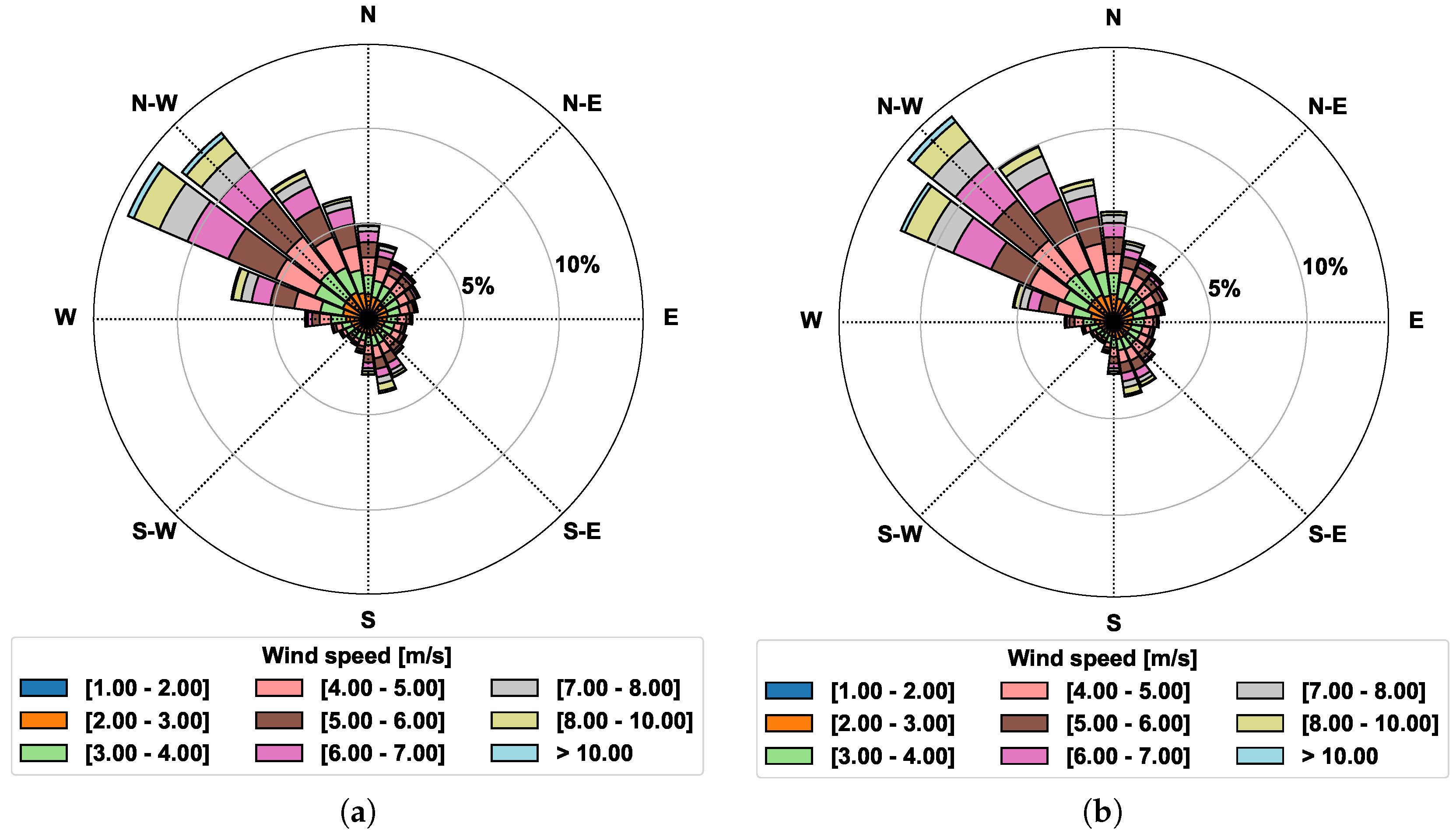
Figure 5.
Top panel: time series of the wind speed (red) and the dynamical running averaged wind speed (blue). Bottom panel: time series of the wind direction (red) and the dynamically averaged wind direction (blue).
Figure 5.
Top panel: time series of the wind speed (red) and the dynamical running averaged wind speed (blue). Bottom panel: time series of the wind direction (red) and the dynamically averaged wind direction (blue).
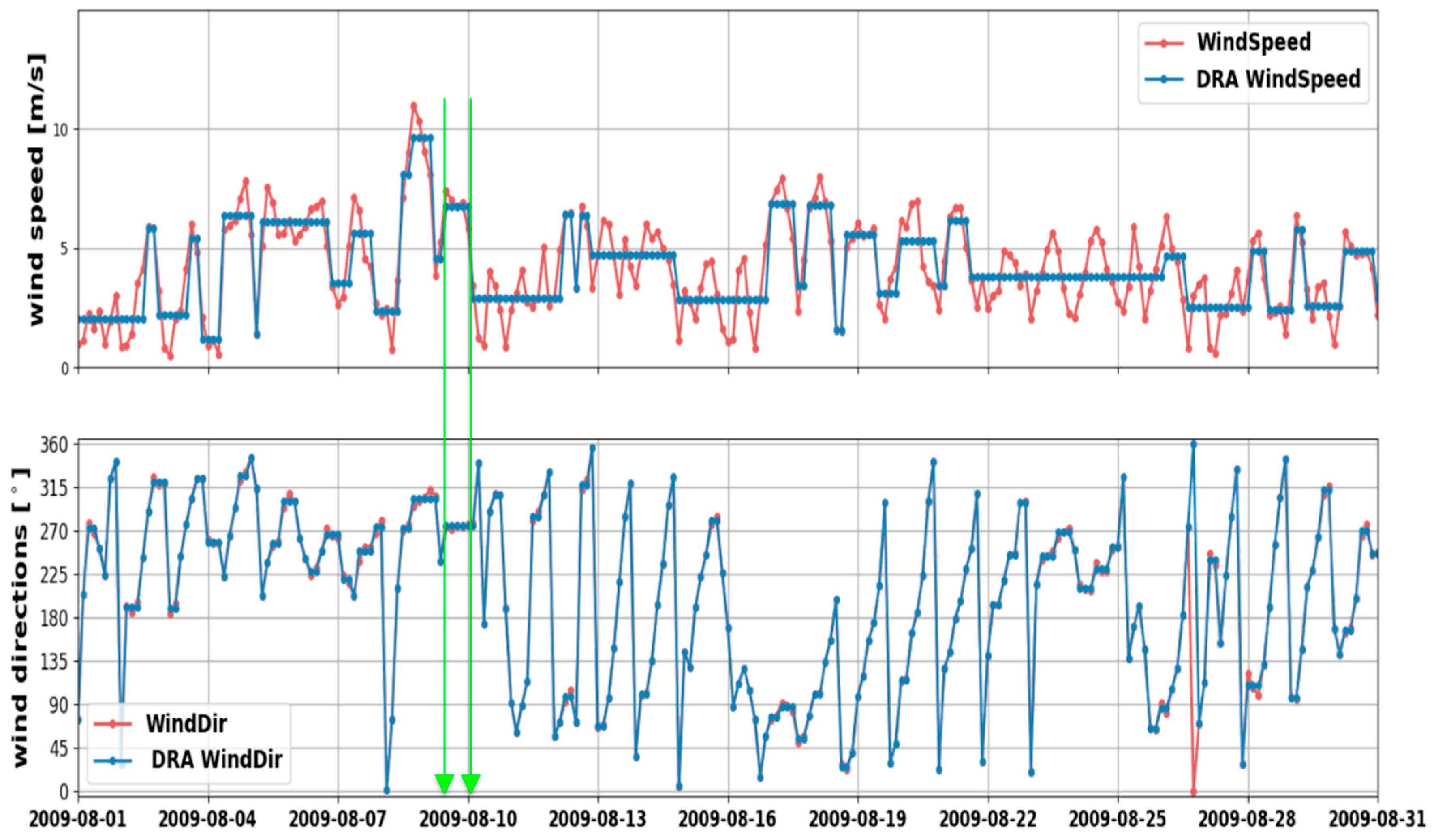
Figure 6.
Determination of the duration of the steady wind generating the waves (zoom of Figure 5).
Figure 6.
Determination of the duration of the steady wind generating the waves (zoom of Figure 5).

Figure 7.
Wave period distribution (normalized p.d.f.) by ADMins, by NOAA and ECMWF datasets and by SPM ’84.
Figure 7.
Wave period distribution (normalized p.d.f.) by ADMins, by NOAA and ECMWF datasets and by SPM ’84.
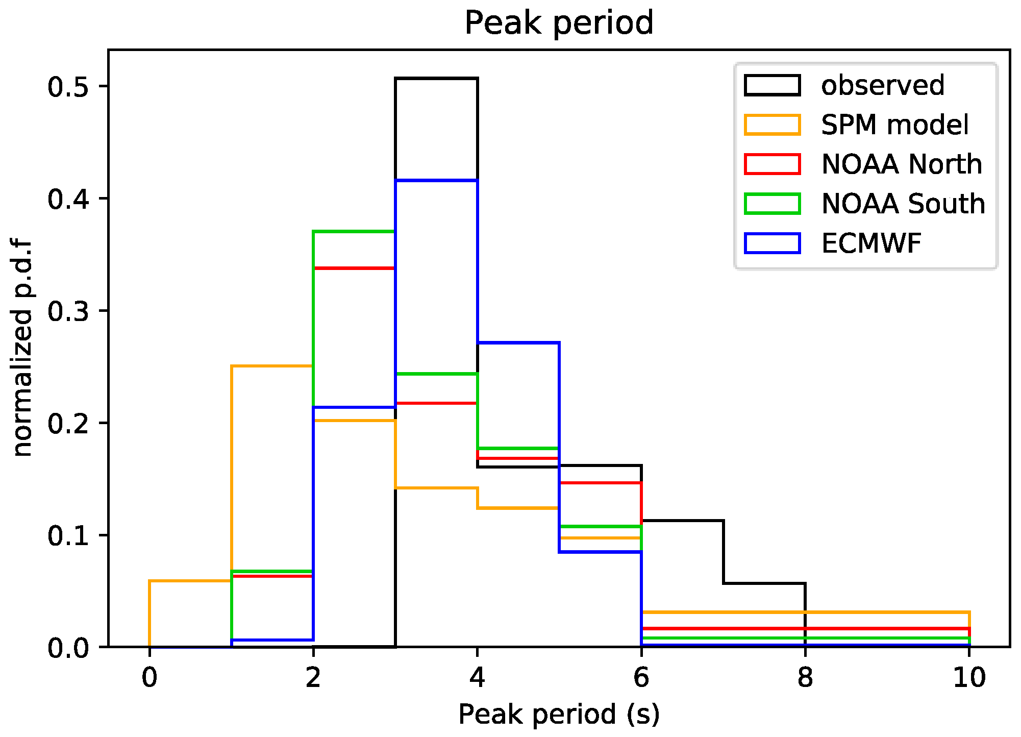
Figure 8.
Wave roses from SPM ’84 (a) and from ADMins (b).

Figure 9.
Difference in values of appearance frequency determined by SPM ’84 and observed by ADMins.
Figure 9.
Difference in values of appearance frequency determined by SPM ’84 and observed by ADMins.

Figure 10.
NOAA wave rose at the north node (a), NOAA wave rose at the south node (b), and ECMWF (c) wave rose in proximity of the ADMins.
Figure 10.
NOAA wave rose at the north node (a), NOAA wave rose at the south node (b), and ECMWF (c) wave rose in proximity of the ADMins.
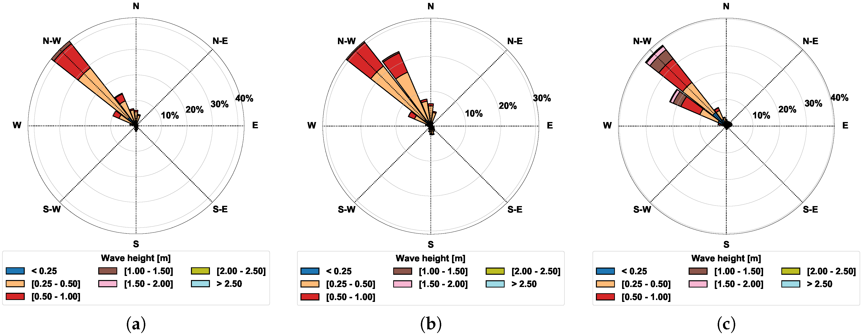
Figure 11.
SWAN-computed wave rose at the ADMins location.

Figure 12.
Scatter plots of each hindcasted model af versus the observed af.
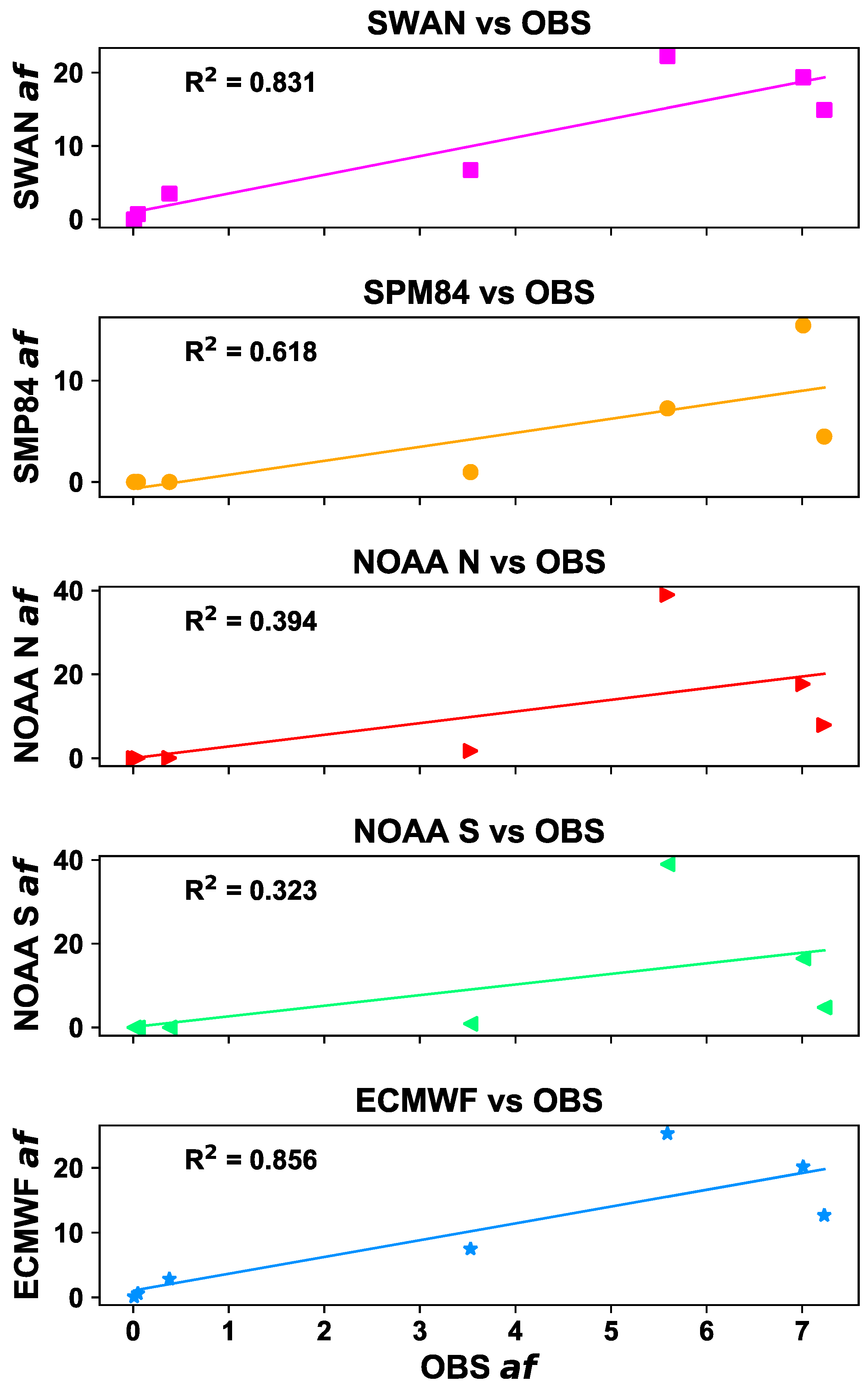
Figure 13.
Taylor diagram of the performance of each of the considered models.


Table 1.
ADMins, NOAA N, NOAA S, ECMWF, NOAA Offshore coordinates, and water depths.
| Name | Longitude (°E) | Latitude (°N) | Water Depth (m) |
|---|---|---|---|
| ADMins | 54°24′29″ | 24°34′17″ | 6 |
| NOAA North | 54°30′00″ | 24°40′00″ | 6 |
| NOAA South | 54°19′59″ | 24°30′00″ | 3 |
| ECMWF | 54°22′30″ | 24°37′30″ | 11 |
| NOAA Offshore | 54°00′00″ | 25°00′00″ | 21 |
Table 2.
Main SWAN configuration parameters.
| Model Version | SWAN 41.20 |
|---|---|
| Time and Spatial mode | Stationary 2-dimensional |
| Bathymetry | GEBCO_2014 (30 arc-second) |
| Computational domain | LON: 54.00417° E, 54.59584° E |
| LAT: 24.00417° N to 25.00417° E | |
| 71 × 120 computational nodes | |
| Wave frequency grid | 0.04 to 1.00 Hz, 24 frequencies |
| Directional grid | 0° to 360°, 36 directions |
| Physics | |
| Breaking | constant breaker index, γ = 0.73 |
| Whitecapping | Komen et al., 1984 [50] |
| Bottom Friction | Madsen et al., 1988 [43] |
| equiv. roughness length scale of the bottom 0.001 m | |
| Triads | included |
| Diffraction | excluded |
| Quadruplets | excluded |
| Boundary conditions | N boundary: from 54.00417° E to 54.59584° E |
| provided by NOAA WW3 | NNW boundary: from 24.834° N to 25.00417° N |
| Boundary wave spectra shape | Jonswap [51] |
Table 3.
Bathymetry and the computational resolution.
| Name | Bathymetry | Computational Grid | Output Grid | |
|---|---|---|---|---|
| Name | Resolution | Resolution | Resolution | |
| NOAA | ETOPO-1 (1 arc-minute resolution) | 10 arc-minutes = 1/6° (interpolated) | 10 arc-minutes = 1/6° (interpolated from 1/2°) | 10 arc-minutes = 1/6° (interpolated from 1/2°) |
| ECMWF | ETOPO-2 (2 arc-minute resolution) | 2 arc-minutes = 1/30° | 80 km | 1/8° (interpolated from T255) |
| SWAN | GEBCO | 30 arc-seconds = 1/120° | 30 arc-seconds = 1/120° | 30 arc-seconds = 1/120° |
Table 4.
NW af, for classes of Hs.
| Dataset | Classes of HS (m) | ||||||
|---|---|---|---|---|---|---|---|
| [0, 0.25] | [0.25, 0.5] | [0.5, 1.0] | [1.0, 1.5] | [1.5, 2.0] | [2.0, 2.5] | >2.5 | |
| ADMins (O) | 7.23 | 5.59 | 7.01 | 3.53 | 0.38 | 0.05 | 0.01 |
| SWAN | 14.88 | 22.25 | 19.33 | 6.68 | 3.48 | 0.70 | 0.00 |
| SPM ’84 | 4.48 | 7.26 | 15.45 | 0.97 | 0.00 | 0.00 | 0.00 |
| NOAA N | 7.90 | 38.99 | 17.63 | 1.68 | 0.03 | 0.00 | 0.00 |
| NOAA S | 4.76 | 39.01 | 16.47 | 0.86 | 0.00 | 0.00 | 0.00 |
| ECMWF | 12.66 | 25.29 | 20.16 | 7.49 | 2.85 | 0.59 | 0.10 |
Table 5.
Wave model errors’ statistical indicators.
| Dataset | af BIAS | af RMSE | af NBIAS | af NRMSE | af SMAPE | af SRMSE |
|---|---|---|---|---|---|---|
| SWAN | 6.22 | 8.52 | 3.84 | 5.98 | 1.25 | 1.35 |
| SPM ’84 | 0.62 | 3.55 | -0.37 | 0.86 | 1.23 | 1.42 |
| NOAA N | 6.06 | 13.27 | 0.59 | 2.42 | 1.27 | 1.44 |
| NOAA S | 5.33 | 13.20 | 0.46 | 2.43 | 1.42 | 1.54 |
| ECMWF | 6.48 | 9.36 | 4.80 | 6.07 | 1.19 | 1.27 |
© 2018 by the authors. Licensee MDPI, Basel, Switzerland. This article is an open access article distributed under the terms and conditions of the Creative Commons Attribution (CC BY) license (http://creativecommons.org/licenses/by/4.0/).
Share and Cite
MDPI and ACS Style
Hamza, W.; Lusito, L.; Ligorio, F.; Tomasicchio, G.R.; D’Alessandro, F. Wave Climate at Shallow Waters along the Abu Dhabi Coast. Water 2018, 10, 985. https://doi.org/10.3390/w10080985
AMA Style
Hamza W, Lusito L, Ligorio F, Tomasicchio GR, D’Alessandro F. Wave Climate at Shallow Waters along the Abu Dhabi Coast. Water. 2018; 10(8):985. https://doi.org/10.3390/w10080985
Chicago/Turabian StyleHamza, Waleed, Letizia Lusito, Francesco Ligorio, Giuseppe Roberto Tomasicchio, and Felice D’Alessandro. 2018. "Wave Climate at Shallow Waters along the Abu Dhabi Coast" Water 10, no. 8: 985. https://doi.org/10.3390/w10080985
Note that from the first issue of 2016, this journal uses article numbers instead of page numbers. See further details here.