1. Introduction
For decades, dams have been built and operated mostly for economic purposes that require a reliable water supply for human needs, such as hydropower electricity, irrigation, living and industry water supply, and navigation. Water withdrawn for increasing economic demands has led to conflicts between human water use and ecosystem water needs [
1,
2,
3]. The operation of dams leads to negative effects on aquatic and riparian ecosystem systems [
4,
5,
6]. The alteration of the flow regime caused by reservoir operation is recognized as a major driving factor that threatens the integrity of the river ecosystem [
7,
8,
9,
10,
11]. Bunn and Arithington reviewed the studies focused on the relationship between hydrological flow regime and river ecosystems, and illustrate four critical negative impacts of the alteration: (1) alteration of the magnitude of flow as the determinant of physical habitat and biotic composition; (2) alteration of the timing and frequency of peak flow as key factors of the life history of aquatic species; (3) destruction of the patterns of longitudinal and lateral connectivity for riverine species; and (4) the extinguishing of extreme low flow avoidance, meant to prevent the invasion of exotic species [
12].
How to balance the trade-off between humans and ecosystems has been discussed for decades regarding integrated river basin management [
13,
14,
15,
16]. Many investigations have been conducted to address the conflicts between environmental flow release and the economic water supply over the past decades. To evaluate the ecological objective for aquatic and riparian ecosystems’ sustainability, four kinds of approaches are often applied, including (1) estimating the minimum flow requirement for downstream habitats to maintain the survival of specific species [
17,
18,
19]; (2) determining a flow regime based on fish diversity information [
20]; (3) providing a regime-based, prescribed flow duration curve that considers floods and droughts for species and morphological needs [
21,
22,
23]; and (4) minimizing the degree of flow alterations in order to maintain the stability of river ecosystems and population structures of species [
16,
24,
25,
26]. In these studies, it is can be found that the adopted ecological objectives have been shifted from an emphasis on a minimum flow requirement or single species to the development of a regime-based comprehensive approach. With the first two methods mentioned above, the flow fluctuation, which decides the ecological integrity, is generally neglected. Therefore, ecologists currently prefer to recommend the last two methods, in which the ecological integrity can be sustained by accounting for the functional and structural requirements for aquatic and riparian ecosystems.
Suen and Eheart proposed a multi-objective model based on the ecological flow regime paradigm, which incorporates the intermediate disturbance hypothesis to address the ecological and anthropic need [
16]. Their study uses parts of the Taiwan Eco-Hydrology Indicators System (TEIS) as the criteria to represent ecosystem objectives. Lane et al. proposed a multi-step re-operation methodology to address environmental flow requirements and human water use objectives [
23]. This model summarizes the environmental flow requirements on the basis of empirical streamflow thresholds for the maintenance of an ecosystem with geomorphic functions. Using a one-dimensional water routing model by the Water Evaluation and Planning System (WEAP), the model develops an alternative reservoir rule curve and suggests the new timing of releases to sustain key ecological and geomorphic functions. Generally, these studies have used a monthly-based interval and have therefore failed to reflect important hydrological factors with daily variations, which may play an important role for sustaining the health of an ecosystem [
7,
27,
28,
29]. Chen et al. proposed a time-nested approach, in order to scale down the decision variables from a monthly to a 10-day basis, and further to a daily basis for reservoir operations [
30]. They used a daily flow hydrograph as a constraint in the optimization model. However, the model was extremely complex, with 730 decision variables, leading to a high cost of calculation in the optimization process. Considering daily scale indicators in reservoir operations, such as the timing and frequency of peak flow, the rising and falling rates requires a large number of decision variables in the optimization process, and lead to a computing-heavy task.
It has been noted that involving a set of fixed operation rules in reservoir modelling can reduce the number of decision variables as well as the computational costs [
31]. Standard operating policy (SOP) and hedging rules (HR) are the most commonly used rules in reservoir operations. SOP, which is the traditional and simplest operating rule, releases water as close to the delivery targets as possible in order to meet the demands of the current stage [
32]. By contrast, HR prefers to keep a certain proportion of available water in the reservoir, in order to minimize the possible losses caused by water shortages in the future. Usually, SOP is recommended only if the objective function is linear, while the hedging rules have been proven to be a more efficient way to optimize the reservoir operations when the supply benefits are nonlinear [
33,
34]. In real operations, the trade-off analysis of multiple objectives is often complicated with nonlinear systems and uncertain inflow conditions [
35,
36,
37]. Therefore, HR is often used to cope with uncertain future inflows among different nonlinear objectives in practice [
38]. Taghian et al. employed HR to achieve the optimal water allocation, in order to reduce the intensity of severe water shortages [
39]. A hybrid model was developed to simultaneously optimize both the conventional rule curve and the hedging rule. Shiau developed a parameterization–simulation–optimization approach for optimal hedging for a water supply reservoir by considering the balance between beneficial release and carryover storage value. The proposed methodology was applied to the Shihmen Reservoir in northern Taiwan to illustrate the effects of derived optimal hedging on reservoir performance in terms of shortage-related indices and hedging uncertainty [
40]. Yin et al. used a typical approach that uses three limit curves to divide the reservoir storage and the reservoir inflow into several zones [
24]. A series of water supply rules and water releasing rules were derived by the actual reservoir storage and the reservoir inflows to provide the water supply and to satisfy the ecological needs of seasonally variables, such as base flows, dry season flow recessions, high-flow pulses, etc. However, daily interval variations were not exactly considered in the above-mentioned studies.
Accounting for the daily variation of downstream flows, Yang et al. proposed a set of linear rules to generate daily reservoir releases, with the aim of satisfying the needs of ecological assessment [
20]. This method can explicitly engage flow regime variation based on real-time inflow information [
41], while short-term inflow information becomes crucial for reservoir operation when daily scale ecologic indicators are considered. However, the proposed operation rules were based on traditional operation curves for flood control and ecologic objectives, without further considerations regarding the balance between consumptive water supply and ecological flow needs. Moreover, the ecologic objective in this paper was calculated by seven indicators, including
Q3 and
Q5, the average discharges in March and May, respectively;
Q3day min and
Q7day min, which represent the annual minimum average of three- and seven-day discharges;
Q3day max, which is the annual maximum average 3-day flow; and
Dmin, representing the Julian date of the annual minimum daily flow. Further information, such as the changing trends of daily flow and the statistics of daily flow reversals, are required to establish a more comprehensive function for the ecological objective.
The purpose of this study is to develop practical hedging rules for reservoir operation with economic and ecologic objectives, which will be able to reflect daily interval variations and engage the real-time daily inflow forecast and storage information simultaneously into decision-making. In this paper, piecewise-linear hedging rules are proposed in order to generate the daily release for ecological and economic objectives, through which the parameters are optimized based on historical and synthetic streamflow series. In additional, the objective of ecological flow requirements is quantified by 33 hydrologic parameters from Indicators of Hydrologic Alteration (IHA). The proposed methodology is applied to a realistic reservoir as a performance test. The rest of this paper is organized as follows.
Section 2 briefly introduces the structure of the model.
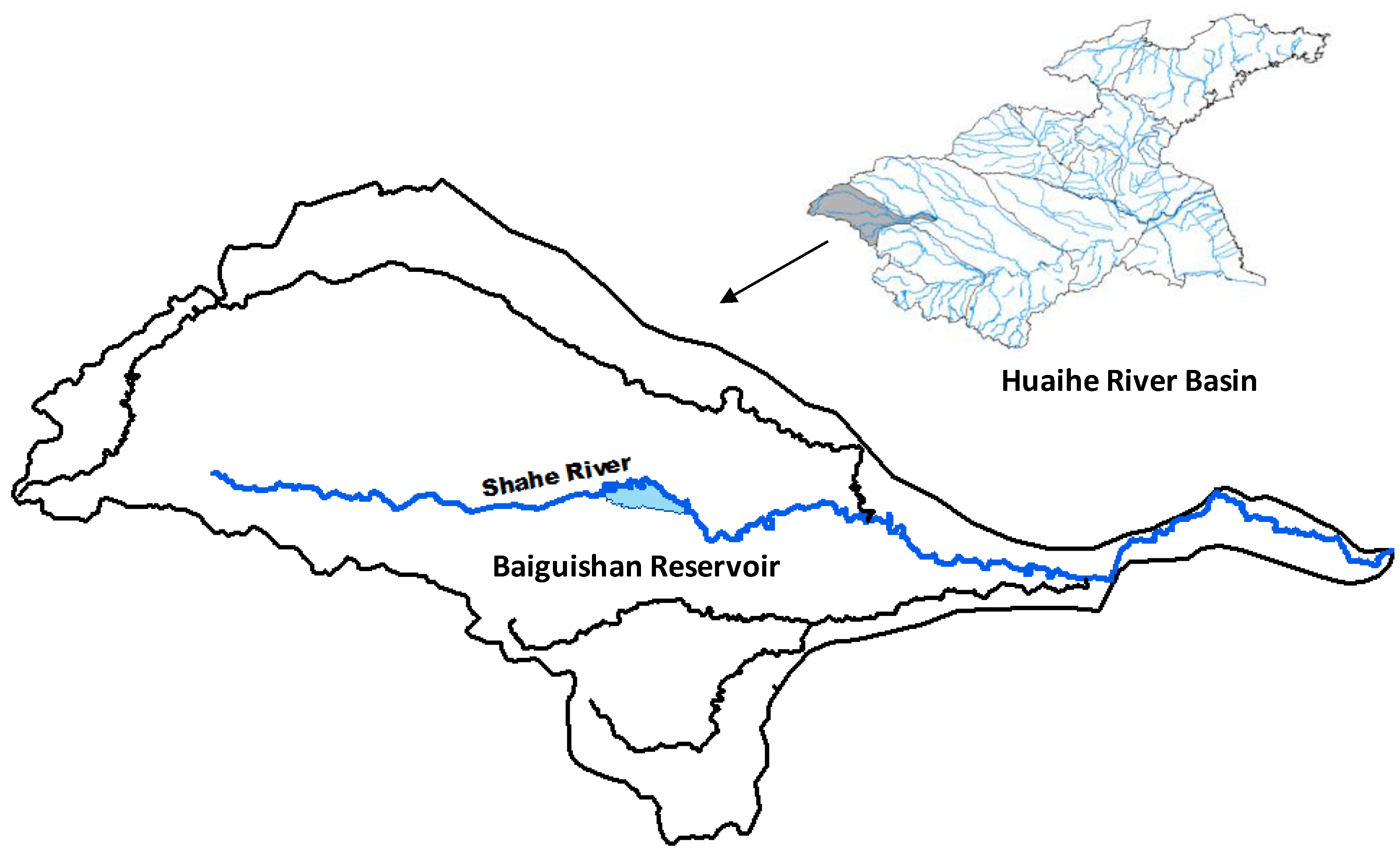
Section 3 presents a real world case study of Baiguishan reservoir, China.
Section 4 compares the proposed HRs with SOP and analyzes the value of forecast information. Finally, conclusions are drawn in
Section 5.
2. Methodology
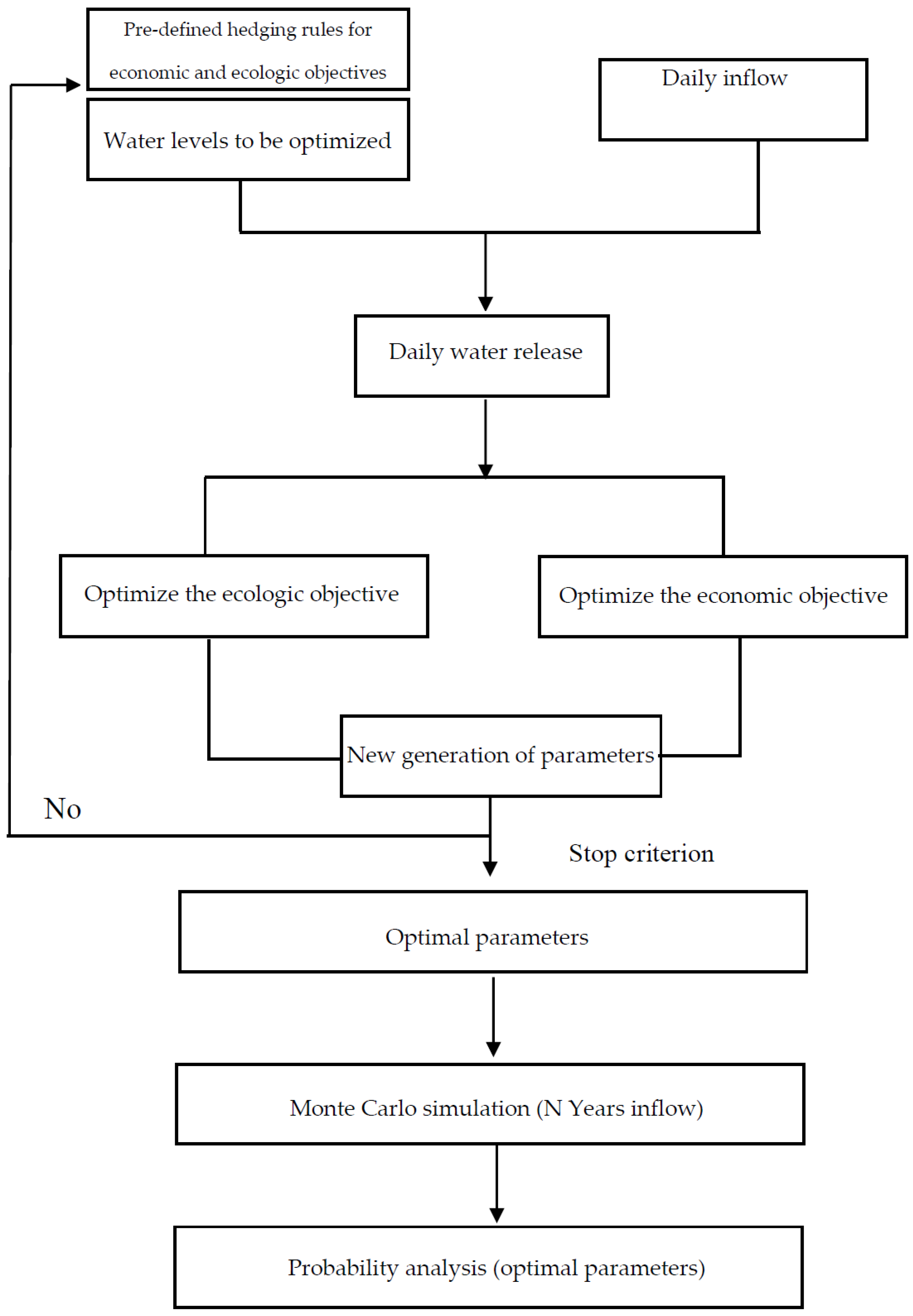
The framework of the method for optimizing the reservoir’s target water levels and flows released to the economic and ecological objectives is shown in
Figure 1. It is composed of the following three steps: (1) generating daily water release based on daily inflow and pre-defined hedging rules, (2) multi-objective optimization for releasing water to economic and ecologic objectives, (3) Monte Carlo simulation and probability analysis to identify the variations of the optimal water release in various hydrological years.
The aim of this framework is to identify a set of practical operating rules for water release. A set of pre-defined, piecewise-linear hedging rules are used to generate water release under the conditions of various inflow and water levels of the reservoirs. A multi-objective genetic algorithm is then applied to optimize the parameters of the rules’ curves iteratively, by balancing the economic and ecological objectives of water release. The statistical characteristics of the parameters are obtained through Monte Carlo simulations, in which the historical and synthetic daily inflows are used as the inputs.
2.1. Pre-Defined Piecewise-Linear Hedging Rules
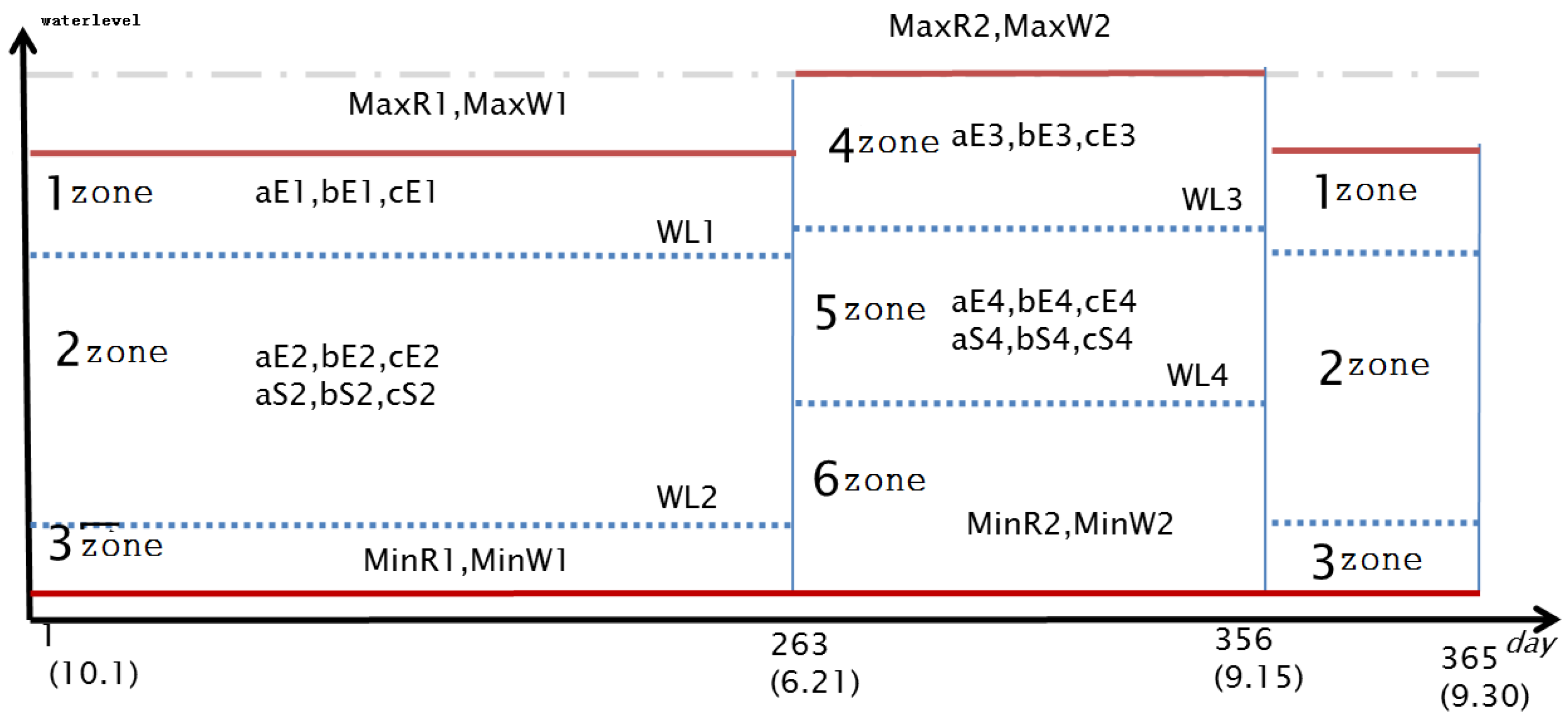
In this paper, piecewise-linear hedging rules considering both economic and ecological objectives are pre-defined for the dry and wet seasons separately. As shown in
Figure 2, zones 1–3 represent the rules in the dry season, and zones 4–6 stand for the rules during the wet season. Red lines show the maximum and minimum water level of different periods following the traditional operation rules currently used by the reservoir.
For the dry season, daily water release for economic objectives can be defined as a set of piecewise-linear hedging rule functions incorporating actual storage and future inflow while considering the effect of daily inflow forecast [
42], as follows:
where
Wt is the water release for economic objective of day
t;
Dt is the target release for economic objective of day
t;
It is the inflow of day
t;
Lt and
Lt−1 are water levels of day
t and day
t − 1, respectively;
WL1 and
WL2 stand for upper and lower limits of the water level, respectively;
MinW1 represents the minimum release for the economic objective of day
t;
aS1,
bS1, and
cS1 are the coefficients of the linear functions of hedging rules.
Specifically, when the actual water level (Lt) is higher than the upper limit (WL1), it implies that the stored water is enough to defend the area from droughts in the future. In this case, the economic water release Wt can be described as the amount of water that is needed (Dt). When the actual water level (Lt) is between the upper limit (WL1) and the lower limit (WL2), it means that there is insufficient storage to defend against future droughts, and thus the water release Wt can be described as a linear function related to the forecasted inflow and current water level. When the current water level is lower than the lower limit (WL2), it means that storage is rare and there is a huge drought risk in future. In this case, Wt is defined as a fixed minimum value, representing the minimum or basic water release to the economic system.
Similar to Equation (1), the daily water release for an ecologic objective is defined as follows:
where
Rt represents the ecological water release of day
t;
aE1,
bE1,
cE1,
aE2,
bE2, and
cE2 are the parameters of the HR, which will be obtained through the optimizations illustrated in
Figure 1;
MaxR1 and
MinR1 are the maximum and minimum water release that need to be optimized, respectively.
Similarly, economic and ecological water releases in wet seasons can be defined as follows:
where
WL3 and
WL4 are the upper and lower limit, respectively;
MaxR2 and
MinR2 are maximum and minimum water release to be optimized, respectively; and
aS2,
bS2,
cS2,
aE3,
bE3,
cE3,
aE4,
bE4, and
cE4 are the parameters of the HR during wet seasons.
Consequently, the decision variables consist of the following three parts: (1) water level limits (WL1 and WL2 in dry seasons and WL3 and WL4 in wet seasons); (2) ecological and economic hedging coefficients (aE1, bE1, cE1, aE2, bE2, cE2, aE3, bE3, cE3, aE4, bE4, cE4 aS2, bS2, cS2, aS4, bS4, and cS4); and (3) maximum and minimum water release (MinW1, MinW2, MinR1, MinR2, MaxW1, MaxW2, MaxR1, MaxR2).
2.2. Ecological Objective
The ecological objective is to minimize reservoirs’ alterations on rivers’ natural flows, which have been adapted to by aquatic and riparian species over thousands years of evolution by maintaining the stability of ecosystems and population structures of species. The Indicators of Hydrologic Alteration (IHA) program, proposed by Richter, has been adopted to represent the ecological objective in this paper [
4]. It contains 33 hydrologic parameters involving five groups of characteristics, including (1) the magnitude of monthly stream flow; (2) the magnitude of annual extreme flows at different time durations; (3) the timing of annual extreme flows; (4) the frequency and duration of high and low pulses; (5) the rate of change.
For each eco-hydrological indicator, a spectrum of values could be set as the target range, which could reflect the changes of environmental flow regime that a species can adapt to. If the actual value of an indicator falls in that range, it means that the alteration of the natural flow regime is acceptable by the aquatic or riparian species. Those acceptable ranges of all the indicators have been investigated by many researchers [
9], among which the findings by Richter et al. are mostly widely applied through the range of variability approach (RVA) [
4]. RVA is an efficient and convenient method to evaluate the degree of flow regime alteration. According to Richter and in this paper, the 25th and 75th percentiles of the historical annual value of the indicators are set as the upper and lower limits of the target range of environmental flow regime, respectively.
Here, let
fi(
r) represent the effect function of the
i-th indicator of IHA. In addition,
ihai(
r) represents the value of the
i-th indicator.
fi(
r) equals 0 if
ihai(
r) falls in the target range, which implies that the ecological release and flow alternation compared to the natural flow regime are acceptable. When the value of the indicator falls outside of the target range,
fi(
r) is calculated as the distance from the target range, as follows:
where
r is the series of ecological water release generated by Equations (2) and (4);
ihaip25 and
ihaip75 are the upper and lower limits of the annual values of the indicators, respectively; and
ihai(
r) represents the value of the
i-th indicator. The ecological objective can be calculated by the sum of the 33 indicators of the IHA, as
The value of f1, the range of which is greater than zero, represents the ecosystem objective to be minimized in the multi-objective optimization model.
2.3. Economic Objective
The economic objective is represented in a target-hitting form, in which the water demands of agriculture, industry, and domestic water use are considered. For equalizing the water supply shortages across time intervals throughout the year, the economic objective is employed through quantifying the water supply deficits, as follows:
where
T is the total number of time periods;
di is the economic water demand of the
i-th day, including the water demands of agriculture, industry and domestic sectors; and
wi is the water supplied in the
i-th day. The value of
f2, range from 0 to 1, and represents the economic objective to be minimized in the multi-objective optimization model.
2.4. Constraints
Constraints within the optimization model are set as follows.
(1) Water balance constraint:
where
Vi and
Vi−1 represent the reservoir storage available at the end of the
i-th day and
i − 1 day, respectively;
Ii is the inflow of the
i-th day;
qi is the total release during the
i-th day; and
Ei is the evaporation of the reservoir in the
i-th day.
(2) Reservoir storage capacity constraint:
where
and
are the minimum and maximum water level limits at the end of the
i-th day, respectively; and
Li is the water level of the
i-th day.
(3) Initial and end storage constraint:
Considering the initial water storage of next year, here we set up initial storage and end storage equally as
where
V0 is the initial storage of the reservoir and
Va is its end storage.
The multiple objectives of the model are set to meet both the ecosystem and human demand, which can be expressed as follows:
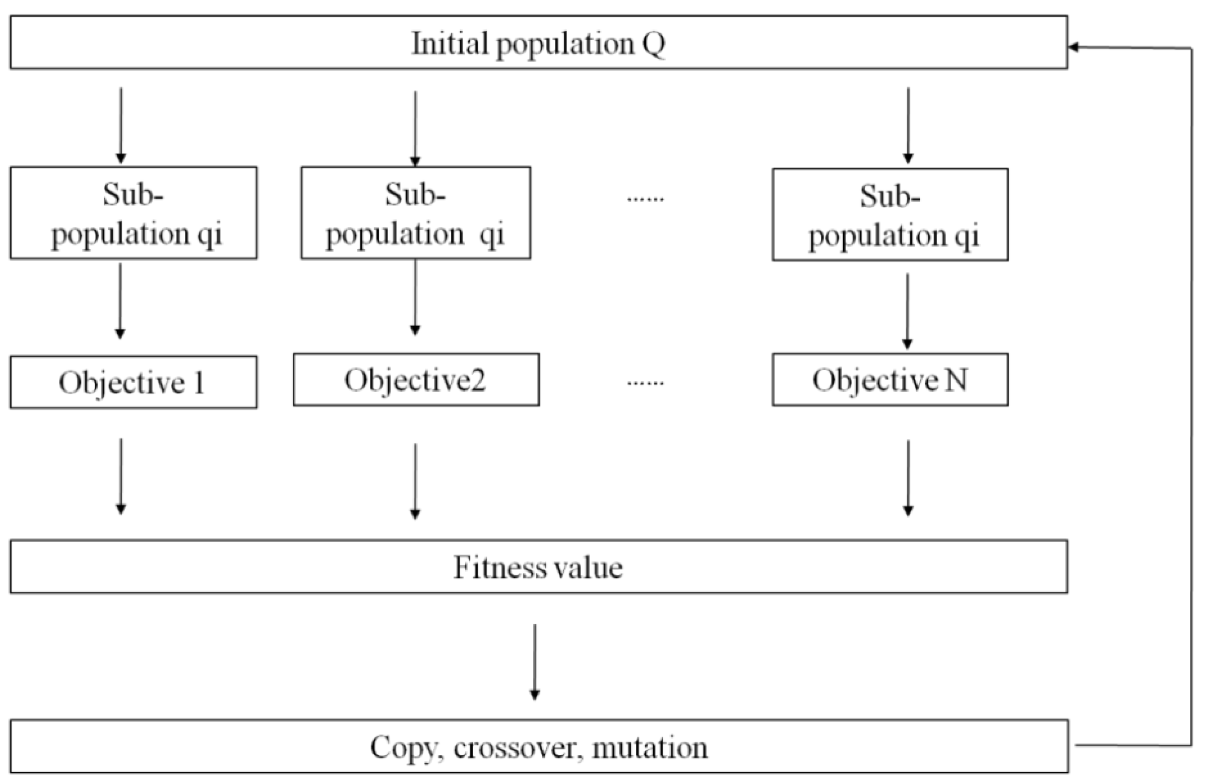
2.5. Vector Evaluated Genetic Algorithm
This multi-objective model is solved by the vector evaluated genetic algorithm (VEGA). Different from the standard procedure of a genetic algorithm, VEGA focuses on the optimization of several objectives [
43]. Through the VEGA, the initial population is divided into a number of objectives, and the elite of each group is selected for the next generation while the others are put in crossover and mutation pools. A population with a higher fitness value has a greater probability of persevering to the next generation. The procedure of VEGA is presented in
Figure 3.
4. Discussion
To test the effectiveness and the robustness of the proposed model, PMHR
B and PMHR
C in
Table 4 were used to generate the economic and ecological water release by which the corresponding objectives were derived. Using the 100 years of synthetic inflows generated in
Section 3.4, the economic and ecological water release processes, as well as the corresponding objectives under different inflow scenarios by the two PMHR rules, were calculated. For comparative study, the economic and ecological water release and their objectives were calculated by the traditional and simplest operating rule SOP, which meant releasing water as close to the delivery targets as possible in order to meet the demand.
4.1. Economic Versus Ecological Objectives under Different Inflow Scenarios
To demonstrate the effectiveness of the HR rules comparing with the SOP rule, the values of economic and ecological objectives optimized by the PMHR
B, the PMHR
C, and the SOP are compared in
Table 5.
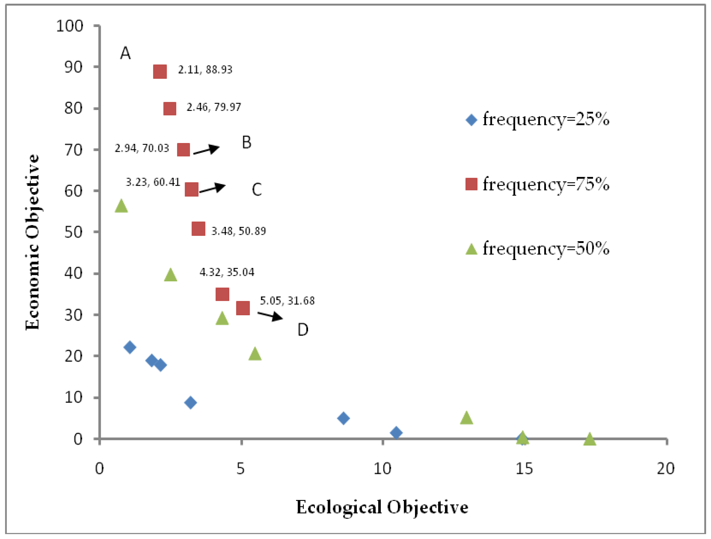
According to Equations (5) and (6), the range of ecological objectives is greater than or equal to 0, and a greater value means a less satisfied ecologic objective. According to Equation (7), the range of economic objectives is from 0 to 1, where a greater value means a higher water supply deficit. With the annual inflow data ranging from a frequency of 10% to 95%, two objective values are compared, as shown in
Table 3.
The SOP can satisfy almost all of the economic water demands under a majority of scenarios, but with a greater alteration to the natural flow regime. For the water supply objective (economic objective), the SOP guarantees meeting 100% of the water demands, except in extremely dry years (frequency = 95%). At the same time, the corresponding ecologic objective is greater than 100, which implies a highly altered flow regime. Meanwhile, PMHRB and PMHRC are able to effectively improve the ecological objective by decreasing the ecologic objectives to the range of 2.66–52.21, and satisfy the economic water demands in wet years (frequency < 50%). In dry years, PMHRB and PMHRC have to reduce the water supply for human demand in order to meet the demands of the ecosystem. For a typical dry year (when the inflow frequency is 75%), PMHRB and PMHRC each reduce nearly 10% of the water supply for human demands in order to balance the ecological objective. When it comes to the extreme dry year (frequency > 95%), PMHRB and PMHRC each reduce about 50% of human water supply to meet the demands of ecosystem.
4.2. Ecological Release
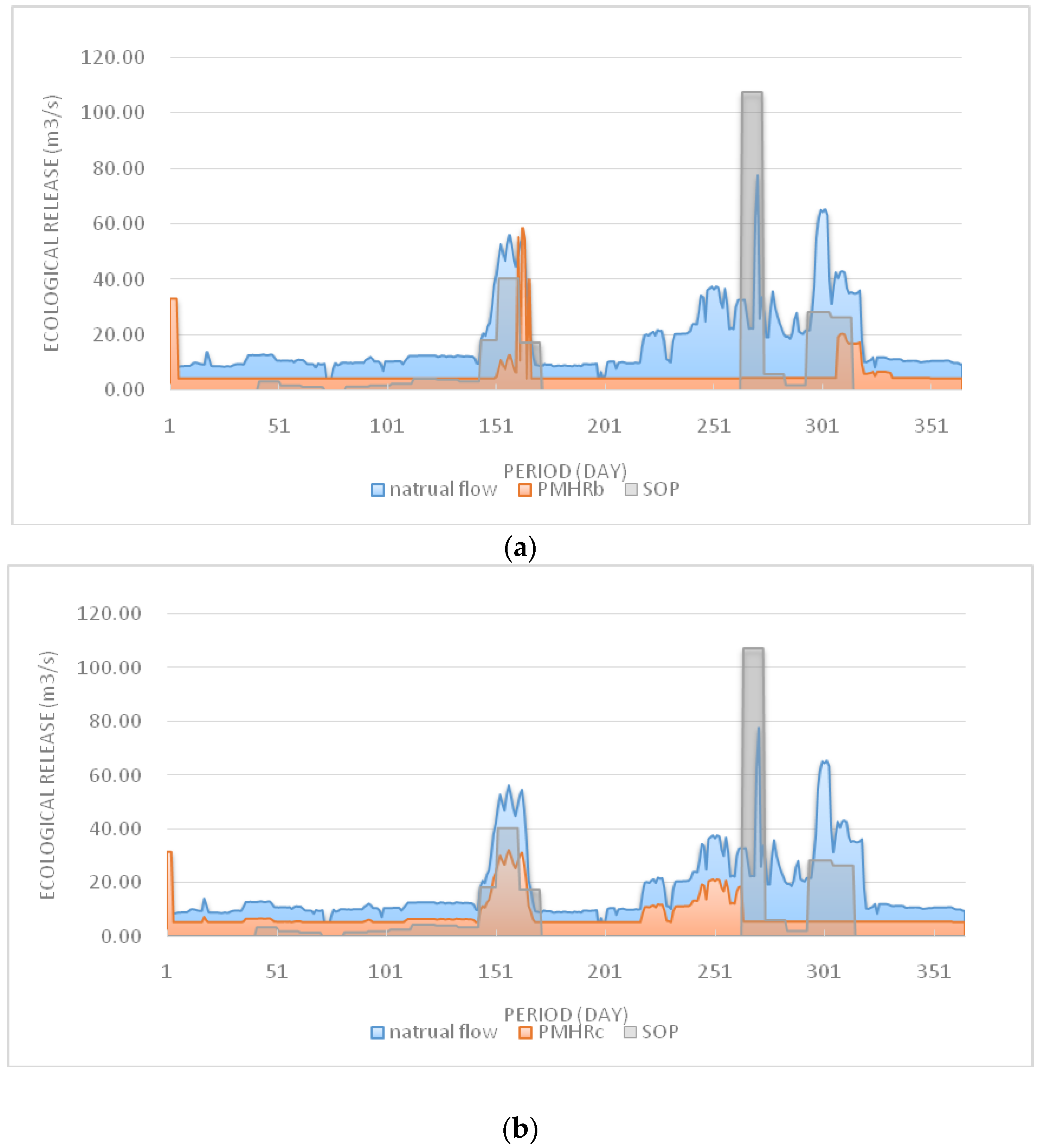
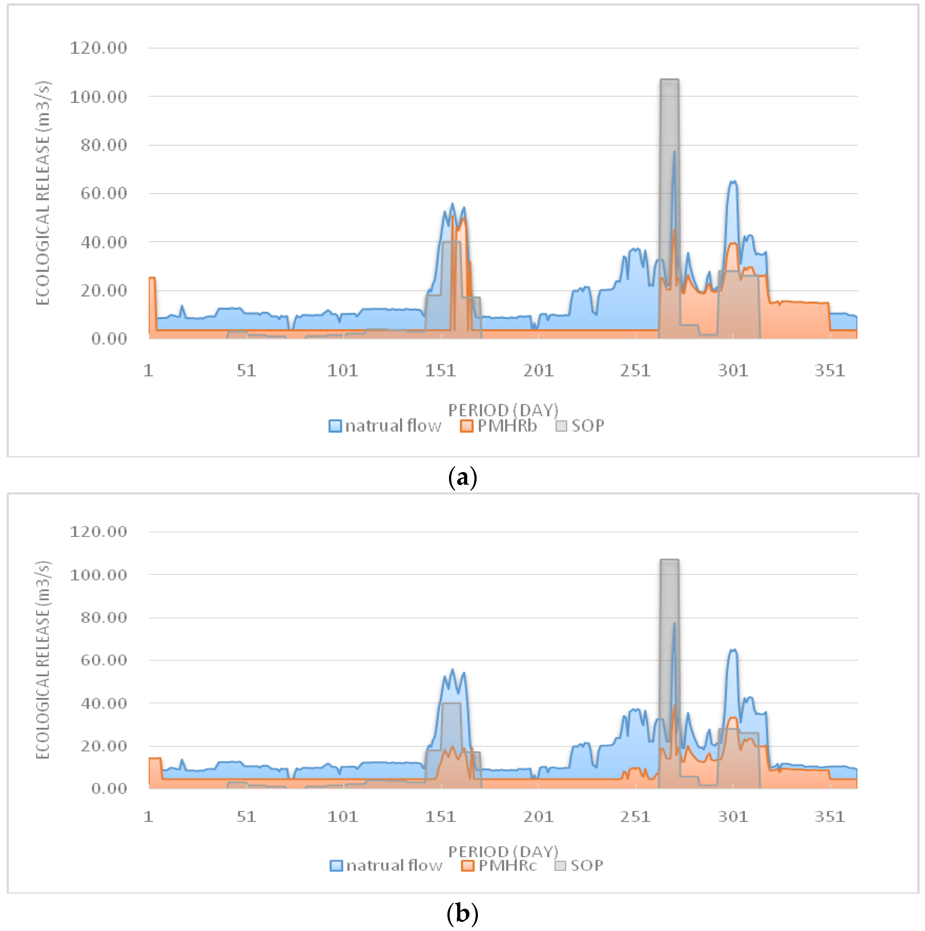
Under the synthetic inflow conditions, the processes of ecological release in a typical dry year (75% frequency), generated by three rules (SOP, PMHR
B and PMHR
C), were compared, as shown in
Figure 6 and
Figure 7. The processes generated by the expected values of PMHR
B and PMHR
C are shown in
Figure 6; processes generated by the median values of PMHR
B and PMHR
C are shown in
Figure 7. Compared to the SOP, the ecological release processes generated by PMHR
B and PMHR
C are closer to the natural inflow process. The similarity of the ecological water release process to the inflow process can be quantified by the correlation coefficient. The higher the correlation coefficient is, the closer the release is to the inflow of the reservoir. This means that the smaller hydrologic alteration is made through reservoir operations. Using
Figure 6 as an example, the correlation coefficient of the inflow and water release under the SOP is 0.54, while the correlation coefficient of inflow and water release under the PMHR
B and PMHR
C are 0.81 and 0.66, respectively.
4.3. Monte Carlo Simulation Key Indicators Analysis
Figure 6 and
Figure 7 demonstrate that reservoir water release alters the flow regime of the river course. This will threaten fish communities and the integrity of river ecosystems downstream. Compared to the operation results under the SOP, the ecological release under the PMHR
B and the PMHR
C can recover the altered flow regime significantly.
The most altered IHA indicators under the SOP are in
Table 6, as well as the indicators under PMHR
B and PMHR
C. The upper and lower limits (25% and 75% frequency of natural distribution, respectively) of each indicator are also listed for reference. If the value of indicators falls within the range of the upper and lower limits, it means a more acceptable ecological condition for sustainability (as the bold number in
Table 6).
4.4. Extended Analysis: Impact of Long-Term Forecast Information
In this section, the impacts of using long-term annual forecast inflows in an operation are discussed preliminarily. We suppose that the annual forecast information, which simply indicates the inflow of the next year and is either larger (wet year) or smaller (dry year) than the average level, is known in advance. Thus, the synthetic inflows used by the Monte Carlo simulation can be divided into two parts: the inflow in wet years and the inflow in dry years. By using the inflow of wet or dry years instead of all the synthetic inflows, the parameters of PMHR can be optimized in two groups: parameters adapted to wet years and parameters adapted to dry years. The expected value of these parameters can be used for wet and dry years, respectively.
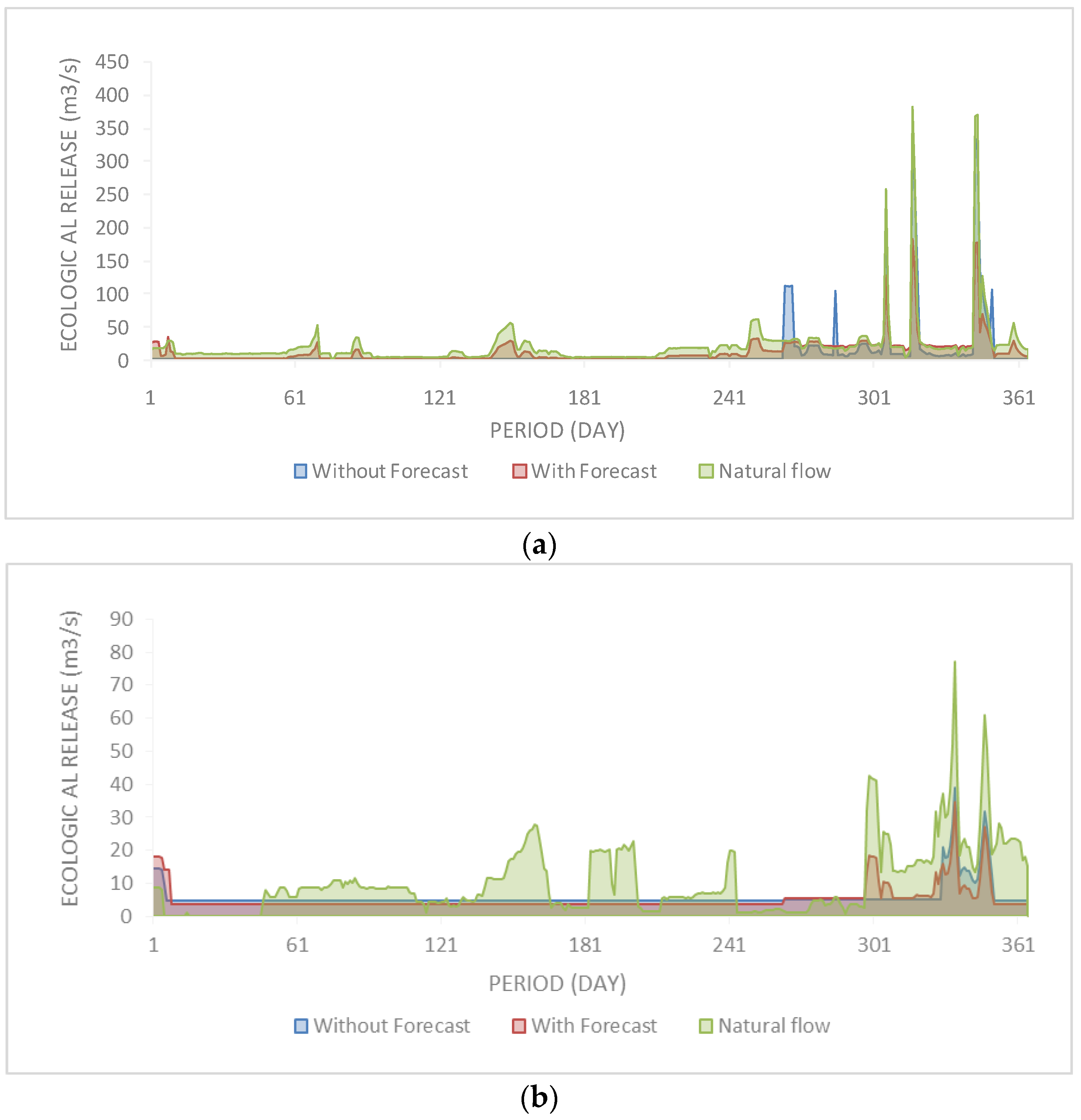
Figure 8 shows the environmental flow release using rules in both wet and dry years with long-term forecast information, as well as the release using rules of all possible hydrological years without long-term forecast information.
Figure 8a presents the results of a typical wet year (frequency = 25%), in which the correlation coefficient between the water release process and the inflow process is 0.95 with forecast information, but 0.90 without forecast.
Figure 8b presents the results of a typical dry year, in which the correlation coefficient is 0.66 with forecast information and 0.61 without forecast information. This indicates that the PMHR combined with forecast information is able to improve the restoration of an ecological flow regime compared to one without the forecast.


