1. Introduction
Water resource scarcity is the most limiting factor for agricultural production in many parts of the world. Mulch has been used throughout the world to increase crop yields and water use efficiency, especially in areas where water resources are scarce. Recently, many biodegradable materials have been used in mulching with great effects, leading many to conclude that mulching will have considerable applications in the future of agriculture [
1]. Plastic film mulching (PM) is currently the principal method that is used for mulch. Many studies have reported that PM significantly improves growth, yield, and water use efficiency (WUE) for many crops, such as wheat [
2], maize [
3], cotton [
4], and sweet pepper [
5] in both rain-fed and irrigated areas.
The objective of using a crop model is to study the impact of agronomic technology, climate, and soil on crop development and growth, yield, and water productivity. The water-driven crop model AquaCrop was developed by the Food and Agriculture Organization of the United Nations (FAO) [
6]. It has a user-friendly interface, provides mulches option, and requires less input data than other crop models [
5,
7]. As a model that is based on crop responses to water, AquaCrop provides better simulation results in crop WUE and soil water content (SWC) than other crop models in the study areas where water is a crucial factor determining yield [
8,
9]. Many studies have indicated that AquaCrop achieved precise modeling results for canopy cover (CC), biomass, yield, and SWC for maize [
10], wheat [
11] and soybeans [
12]. Bello and Walker [
13] tested the AquaCrop model for simulating the CC, biomass, yield, and cumulative evapotranspiration (ETc) of pearl millet under different irrigations and noted good agreement between the simulated and observed data. Few studies have applied the AquaCrop model under PM condition. Malik et al. [
14] tested the applicability of AquaCrop on predicting sugar beet CC, biomass, and root yield under different film mulching and irrigation regimes. Ran et al. [
15] studied the performance of two models (AquaCrop and SIMDualKc) for crop ETc partitioning of maize under PM conditions.
Extreme meteorological events will occur frequently in the future under climate change scenarios [
16]. Thus, the study and projection of agricultural production and water consumption under climate change in arid regions are vital [
17,
18]. Cosic et al. [
5] reported that PM played a significant role in mitigating adverse effects on sweet pepper yields, owing to the extreme weather. Bird et al. [
19] found similar results in the simulation of tomato using AquaCrop. Furthermore, several researchers have noted that crop model calibration is essentially site-specific and simulation performance should be assessed using different field management, climate, crop, and soil to constantly provide suggestions for improving the accuracy and applicability of models [
10,
20]. Therefore, calibrating crop models for more cultivars with and without PM are necessary, and model performance should be evaluated in simulating crop growth and water use under different weather conditions.
Millets, including foxtail millet (
Setaria italica), pearl millet (
pennisetum glaucum), and finger millet (
Eleusine coracana), are widely known as rain-fed crops. They are main food and fodder crop worldwide, particularly in Asia and Africa [
13]. China is the primary consumer and producer of foxtail millet, with a total sowing area of over 150,000 ha [
21]. Because the hybrid foxtail millet “zhangzagu” has many favorable characteristics, such as high yield, drought tolerance, and nutritional value, it has been cultivated over a large area of northern China where the majority of land is rain-fed [
22]. PM is the primary cultivation method for foxtail millet in China [
21]. However, few studies have simulated millets growth using crop models at present [
23].
The main objective of this study was to parametrize and to evaluate the AquaCrop model by using it to simulate growth, water use, and soil water content of foxtail millet grown with and without filming mulching under different weather conditions, to determine whether the model can be used in agricultural production and water management in the north of China.
2. Material and Methods
2.1. Research Area
The experiments were conducted at an innovative agriculture garden in Taigu (37°23′ N, 112°29′ E at 780 m elevation), Shanxi Province, northern China. The experimental region has a typical warm and semi-arid climate, where the mean annual precipitation was 420 mm and the mean frost-free days ranges from 160 to 190 days; the annual accumulated temperature (>0 °C) is 3500 °C.
2.2. Climate Data
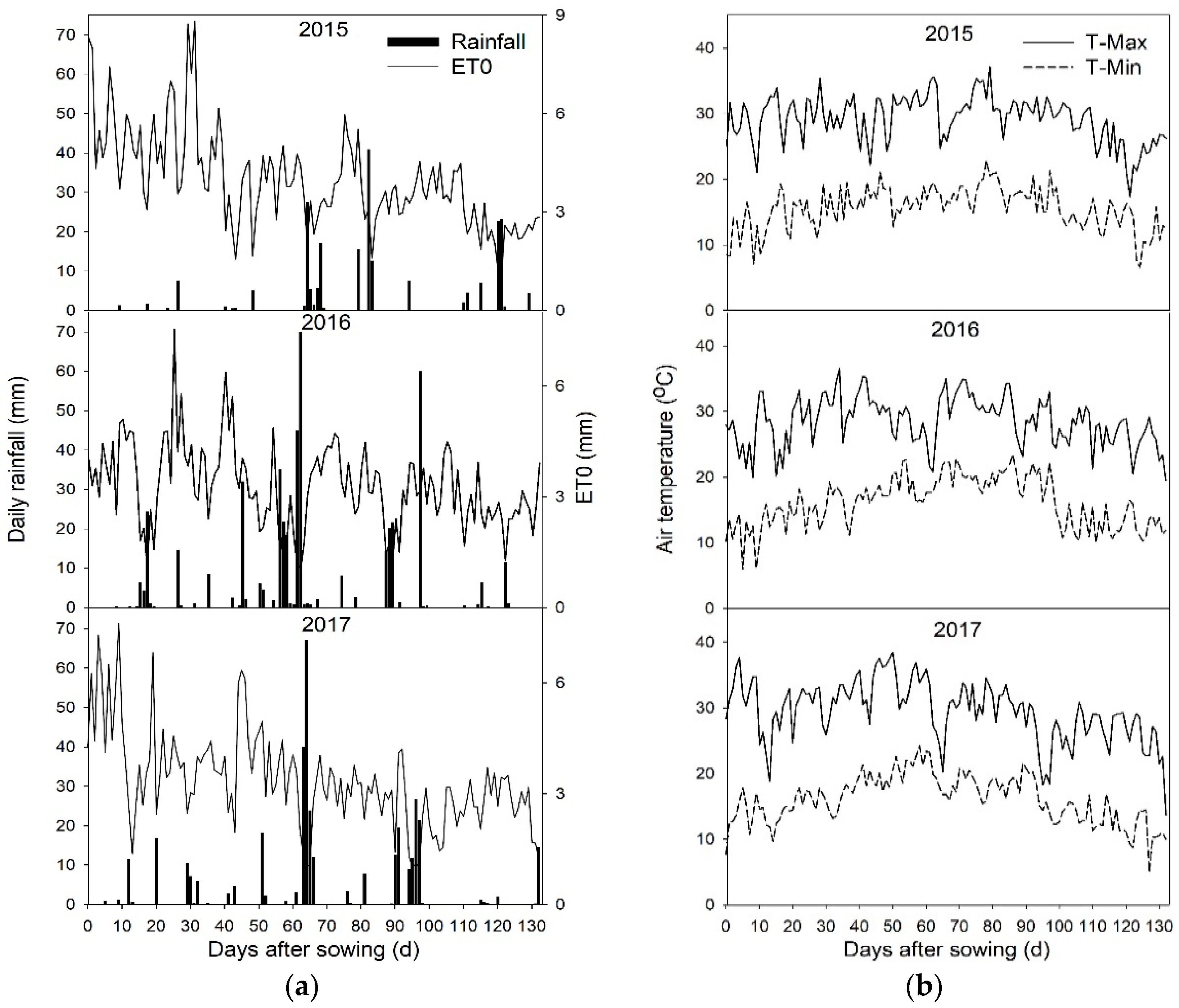
The climate data during the growing period of foxtail millet were obtained from the National Meteorological Information Center of the China Meteorological Administration (
http://cdc.cma.gov.cn/), which included daily precipitation, daily air maximum, and minimum temperatures (
Figure 1). Daily reference evapotranspiration (ETo) (
Figure 1) was calculated by the FAO ETo calculator (
http://www.fao.org/nr/water/eto.html).
The type of rainfall year was determined by using the criteria proposed by Tao et al. [
24], shown as following: Wet year:
dry year:
, where
is the rainfall for year (mm), P is the multi-year (1960–2014) average rainfall (mm), and
is the mean of the squared deviations of each year’s total rainfall from the multi-year average. Because the growing season of foxtail millet runs from May to September, yearly
values were calculated in terms of the precipitation falling during this period. According to the criteria, 2016 was a wet year (total precipitation: 477 mm), 2017 was a normal year (total precipitation: 365 mm), and 2015 was a dry year (total precipitation: 256 mm). Moreover, the daily average temperature during the study period in 2015 was higher than that in 2016 and 2017 by 0.5 and 0.3 °C, respectively (
Figure 1). Especially, the daily average temperature in June 2015 was 1.1 and 0.6 °C higher than the daily average temperature in June 2016 and June 2017, respectively.
2.3. Filed Management and Crop Data
This study employed two treatments: (1) Plastic film mulching (PM) and (2) no mulching (NM). Three years (2015, 2016, and 2017) of field experiments were conducted using a completely randomized block design with five replications. Each plot was 14 m long and 2 m wide with row spacing of 46 cm. Foxtail millet seeds were sown on 12 May 2015, 19 May 2016, and 25 May 2017. The plant density was 340,000 plants ha−1, mulched with flat soil dibbling, and covered by a 0.01 mm thick transparent polyethylene plastic film. Soil cover by mulches was about 50%. On 9 July 2015, all of the plots were irrigated with 45 mm of water due to the severe drought. Manual weeding was adopted in the experimental field. The weed management was excellent in 2015 and 2016 crop season; weeds cover was about 1%. The weed management was good in 2017 crop season; weeds cover was about 10%.
The cultivar of hybrid foxtail millet was “zhangzagu 10”. Each growth stage of foxtail millet was recorded over three years (
Table 1). The growth period of PM treatment and NM treatment in 2015 was three days and one day shorter than those in 2016, respectively. The difference between the length of the growth period of PM and NM in 2017 and those in 2016 is very small.
Canopy cover (CC) was calculated using the empirical relationship between this value and the leaf area index (LAI). LAI was measured every 20 days after sowing using a leaf area meter (CI-230, CID Inc., Camas, WA, USA) on three randomly selected millet plants in each plot. LAI was calculated by dividing the total leaf area by the average ground area per plant. Canopy cover was calculated using Equation (1), as reported in Araya et al. [
25]:
Aboveground biomass was measured every 20 days after sowing. To obtain this, three millet plants were randomly selected from each plot and dried in an oven for 48 h at 105 °C. Three areas of about 2 m
2 (four rows of wide, 1 m long) were randomly harvested from each plot once the millet reached maturity. The ear number, ear grain weight, and 1000-grain weight of millet were measured to calculate the grain yield. Crop WUE was calculated, as follows:
where Y is grain yield (kg·ha
−1) of millet. ETc (mm) was calculated, as follows:
where P is precipitation (mm), I is irrigation (mm), D is deep percolation (mm), R is runoff (mm), and
SW is change of SWC in the 1.6 m soil profile between the planting and harvesting periods. Deep percolation and runoff were assumed as zero based on the experimental condition.
2.4. Soil Data
The organic matter, available nitrogen, available phosphorus, and available potassium in the plow layer of the soil (0–30 cm) were measured with a soil nutrient meter (TPY-6 TOP Inc., Hangzhou, Zhejiang, China), and their contents were 23.79 g·kg
−1, 77.83 mg·kg
−1, 6.81 mg·kg
−1, and 200.35 mg·kg
−1, respectively. The average pH of the soil was 8.16. The soil textural class was determined through the hydrometer method using USDA soil texture classification [
26].
Table 2 lists the soil characteristics of the experimental field, parts of which were obtained from Liu and Zhang [
27]. The Soil Water Characteristics Hydraulic Properties Calculator (
http://hydrolab.arsusda.gov/soilwater/Index.htm) was used to calculate the soil water content at saturation (SAT), field capacity (FC), permanent wilting point (PWP), and saturated hydraulic conductivity (Ksat). The soil water table depth of Taigu is chronically kept five meters below soil surface [
28]. Therefore, the groundwater table of the experimental field was set to 5 m below the soil surface. The capillary rise function was calibrated using the default settings for the selected soil texture and K
sat. Due to the fact that the height of field soil bunds was 0.2 m, the surface run-off curve number (CN) was not applicable [
29]. Readily evaporable water (REW) was set to the default value.
The soil water content was measured using the standard gravimetric method every 15 days after sowing. Samples were obtained by means of a drill with two replicates in each plot, from seven layers: 0–20, 20–40, 40–60, 60–80, 80–100, 100–130, and 130–160 cm.
2.5. Model Calibration and Validation
Farahani et al. [
30] showed that calibration is adjusting some model parameters to make the model match the measured data at the specific location. The AquaCrop required some necessary input data to define the environment in which the crop will develop, including weather, crop, field management, soil, and initial condition data. All of these data were entered into corresponding modules before running the simulation. The input data of the initial conditions in AquaCrop was measured at the start of each experiment. The measured crop data from the field was used as input data for crop development parameters, including plant density, initial canopy cover (CCo), maximum canopy cover (CCx), maximum and minimum effective rooting depth, day to emergence, day to CCx, day to maturity, and day to flowering. Whereas, the remaining crop parameters, such as canopy growth and decline coefficients, were estimated by the model after the input data were entered. Then, these parameters were continuously adjusted to match the measured data for canopy cover, biomass, and yield.
The model was calibrated with measured data from 2016 as the highest yield and biomass were measured in 2016. From the observed data, it can be found that some measured crop data of PM obviously differed from those of NM, such as the growth stage of foxtail millet (
Table 1), initial and maximum canopy cover, and the harvest index. Therefore, it was difficult to adjust the measured crop data that were distinctly different between PM and NM treatments to the input data of one set of crop parameters. So, based on the method from the studies which used AquaCrop to simulate crop growth under PM and NM conditions [
14,
31], we established two sets of crop parameters and corresponding mulching parameters: PM and NM. In the module of field management, AquaCrop provided the option of mulches, where the user could specify the degree of soil cover and the type of surface mulches. Depending on the type of mulches and the fraction of the soil surface covered, the reduction in soil evaporation might be more or less substantial [
32]. At the present study, plastic mulches completely reduced the evaporation of water from the soil surface (100%). The calibration process described by Steduto et al. [
6] was followed for the model calibration. The reference harvest index (HIo) was adjusted to simulate the measured yield in the experimental field. The field management was set at field conditions of non-limiting soil salinity stress and soil fertility stress. A trial-and-error method was adopted to obtain the minimum error values between the simulated and measured data in calibration.
The model was validated through comparing the simulated data with the measured data, as obtained from 2015 and 2017. The indexes evaluated for goodness-of-fit of the model were CC, aboveground biomass, SWC, yield, ETc, and WUE. The AquaCrop version was 6.0.
2.6. Model Performance Assessment
Goodness-of-fit for the calibration and validation of the model was carried out with four statistical indicators: The coefficient of determination (R
2), root mean square error (RMSE), normalized root mean square error (NRMSE), and model efficiency (EF), which were calculated, as follows:
where
and
—simulated and measured values, and
and
—average values of simulated and measured data. That R
2 value gets close to 1 indicated favorable agreement between the simulated and measured values. If the R
2 value > 0.5, it indicated that the simulation results were considered acceptable in watershed simulations [
33].
where n is the total number of observations. As the RMSE value approaches 0, the deviation decreases between the simulated and measured values.
The simulation was labeled (1) excellent, (2) good, (3) fair, or (4) poor for NRMSE values smaller than 10%, between 10% and 20%, between 20% and 30%, or >30%, respectively [
34].
The EF value ranged from 1 to negative infinity with a value of 1 corresponding to a perfect fit.
The data analysis of significant difference used statistics software Statistical Product and Service Solutions (SPSS) (LSD, p = 0.05).
4. Discussion
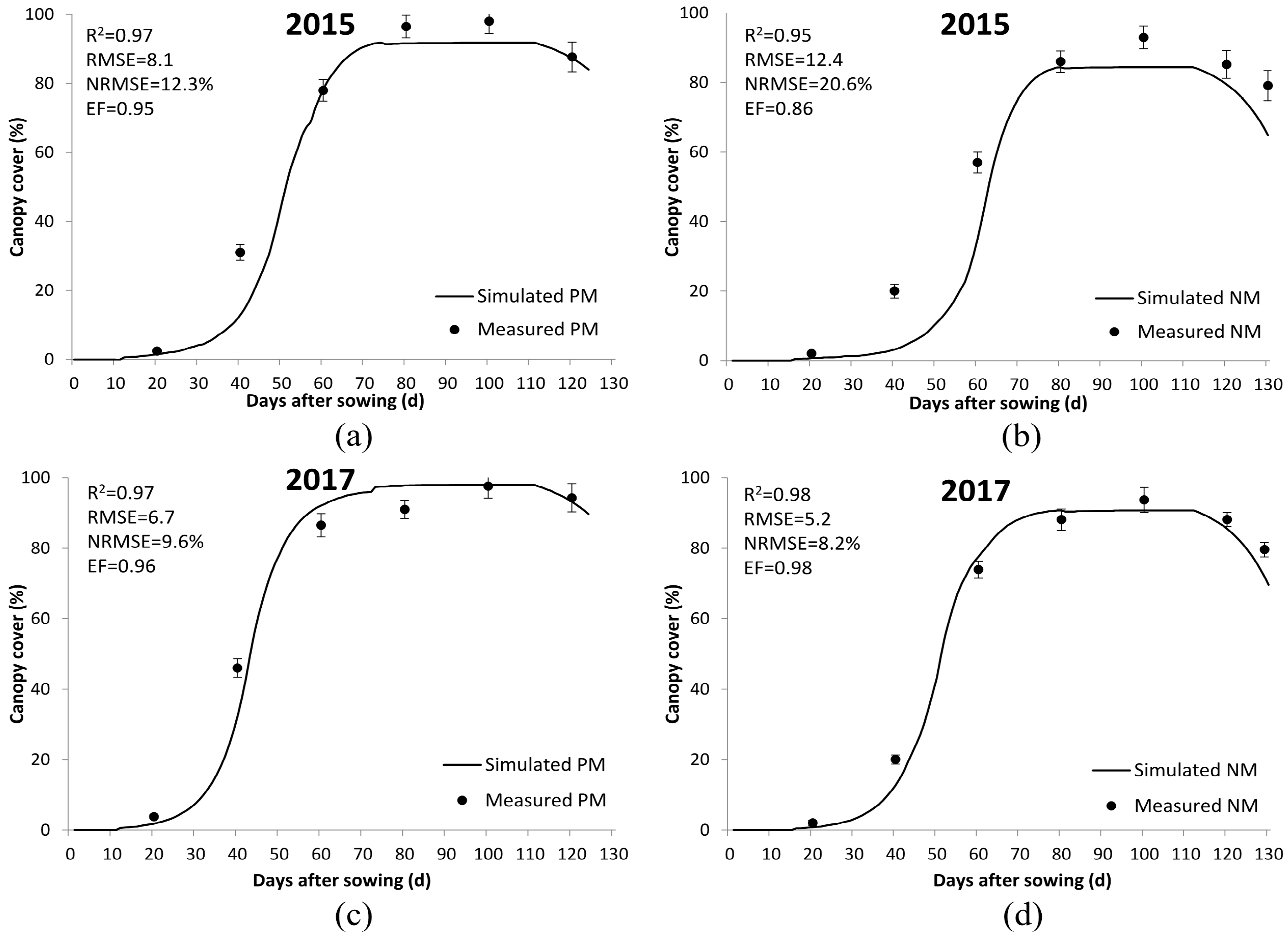
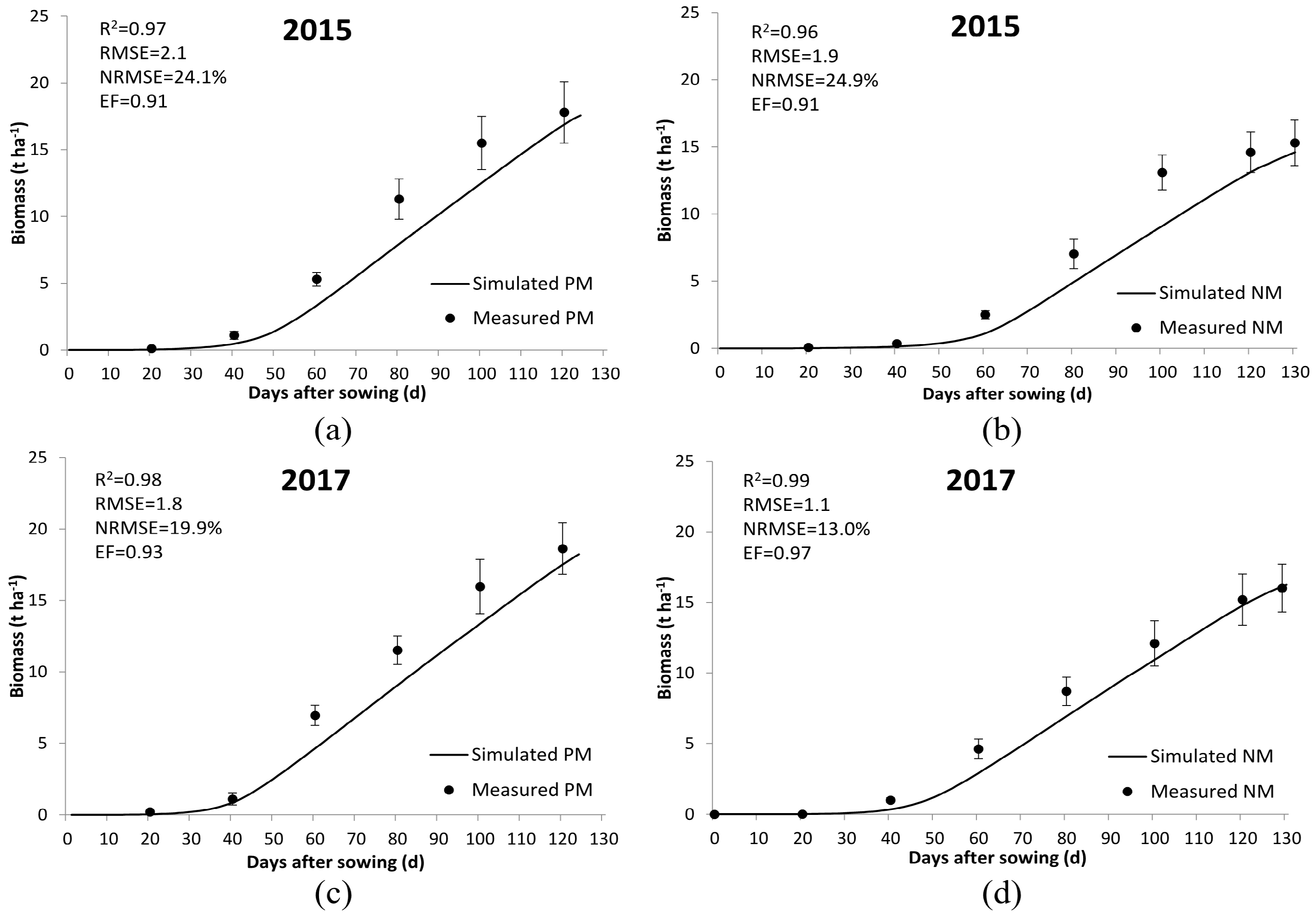
The AquaCrop model achieved accurate predictions for CC development and biomass accumulation of foxtail millet for all treatments, as evidenced by the validation results from 2015 and 2017. The model also effectively simulated the yield of foxtail millet for all treatments in both 2015 and 2017, with small deviations ranging from 2.2% to −5.9%. These results of yield can mainly be attributed to the good simulation for biomass accumulation. Bello et al. [
13] reported similar findings for CC development, biomass accumulation, and yield of pearl millet under different irrigations using AquaCrop. Liu et al. [
35] used AquaCrop to simulated winter wheat under PM and NM conditions and achieved analogous results with this study, which included the R
2 and NRMSE of CC simulation ranging from 0.86 to 0.99 and 2.9% to 11.9%, respectively, and the R
2 and NRMSE of biomass simulation ranging from 0.95 to 0.97 and 18.4% to 42.5%, respectively. Some researchers have pointed out that AquaCrop slightly underestimated the CC and biomass in middle-late crop growth seasons, although the simulation obtained good results, such as with pearl millet [
13] and maize [
10]. Similar results were observed in all the treatments at present study. This could be because of the fact that AquaCrop simplifies the process of crop senescence, especially the process of CC decrease [
36]. Furthermore, the biomass increases of the foxtail millet beyond 63 days after sowing might also have contributed to the underestimation [
37]. Bello et al. [
13] found similar underestimation of biomass in the simulation for pearl millet, and pointed out that this result was due to the biomass accumulation increased beyond 60 days after sowing.
Under different weather conditions, AquaCrop model simulated CC and biomass had varying performance degree. The agreement between the simulated and measured data in 2017 (normal year) was stronger than that for 2015 (dry year). As already mentioned, 2015 was drier and warmer than other years at the study location, which led to the severe water stress during the early growth season in 2015. This severe water stress was assumed to be one of the reasons for the relatively poor agreement that was demonstrated that year. Katerji et al. [
38] tested the prediction of AquaCrop for corn and tomato under various water stress conditions, and wrote that the model performance was demonstrated to vary according to the level of plant water stress. Cosic et al. [
5] simulated the growth of sweet pepper under different weather conditions and noted that “From the above, AquaCrop often fails to produce good results for yield if there is considerable water stress at any time during the growing season.” Studies of maize [
10,
20] and groundnut [
39] also have presented results that would seem to agree with this conclusion. The weather has different effects on the crop growth period, and this influence became more obvious on the crop planting with film mulching [
40]. Under abnormal weather condition in 2015, the observed growth period of foxtail millet was obviously shorter than that of the calibration year (2016). This reduced the accuracy of simulation for CC and biomass in each growth stage using calendar mode. When compared with 2015, the difference between foxtail millet growth period in 2017 and that in the calibration year (2016) was smaller, so, this could be another reason why simulation in 2017 performed preferably to 2015. Additionally, the simulation of CC and biomass for NM generally outperformed than that of PM in 2017, which could be because AquaCrop only considers the change of soil evaporation under PM condition [
32], leading to the effect of soil temperature change on crop growth and soil microorganisms being ignored in the simulation. However, this result was not observed in 2015. PM obtained markedly greater yields and biomass than NM under water stress conditions in 2015, in this case, it was clear that PM played a crucial role in mitigating the adverse impact of drought and high temperatures [
5].
In general, the simulation performance of SWC progression for foxtail millet was acceptable in 2017 for all of the treatments, but it was unsatisfactory in 2015 for both treatments. No consistent conclusion could be derived from the literature regarding the results of simulating SWC using AquaCrop. Andarzian et al. [
11] reported that the model obtained a good result in simulating SWC for different irrigation regimes in Iran. Wang et al. [
8] noted analogous findings for winter wheat in northern China. In the study by Horemans et al. [
41], the AquaCrop model showed good simulation performance for the daily soil water content for a short-rotation coppice application in Belgium. However, the study from Paredes et al. [
12] showed that AquaCrop gave a bias in the estimation of soil water content for simulating soybeans, with a tendency for over-estimation during the first half of the season and under-estimation during the other half. Iqbal et al. [
42] proposed that there was an analogous water-use trend, but there were also certain differences between simulated and measured SWC. Cosic et al. [
5] simulated pepper growth using AquaCrop and observed no strong correlation between the simulated and measured data of SWC under both PM and NM conditions. In the present study, the accuracy of SWC prediction for both PM and NM were improved, which may be due to the use of an effective sampling method (seven soil layers) for SWC and a more precise soil sampling depth for foxtail millet rooting (1.6 m). These methods both reduced the sampling errors, so this study showed an acceptable result for SWC when compared with those unsatisfactory results reported by Cosic et al. [
5]. The simulation performance of CC development and biomass accumulation will greatly influence the simulation of SWC progression [
32]. Better predictions for CC and biomass in 2017 could be one reason for the differences of SWC simulation between 2015 and 2017.
AquaCrop was able to predict ETc and WUE for all treatments in 2017, with acceptable deviations ranging from −4.5% to −10.0%. However, larger deviations were noted under severe water stress in 2015 for ETc (deviations > 14.8%), which could be attributed to the poor simulation of SWC in 2015. This could be because the calculation of ETc is closely related to the simulation of SWC in AquaCrop [
32]. Due to the large deviation of ETc, the simulation results for WUE in 2015 were unsatisfactory. In the study of Katerji et al. [
38] using AquaCrop to simulate maize, the differences among observed and simulated seasonal evapotranspiration became unacceptable in the severely stressed treatments, and the linear regression between the observed and simulated values of WUE was unsatisfactory. Bello et al. [
13] also reported similar results in predicting the SWC and cumulative ETc of pearl millet. The large deviations that were observed from this study revealed that the model requires further improvement in estimating WUE, which is mainly based on evapotranspiration simulation. Deviations between the simulated and actual data of yield, ETc, and WUE in 2017 were generally smaller than those values in 2015. As discussed above in CC and biomass simulation, the model performance declined, as there was severe water stress during crop season, as well as the difference of growth period between 2015 and 2017 all could be contributed to this case. Additionally, the simulation for NM had smaller deviations than that for PM in terms of yield, ETc, and WUE in the normal year (2017). Analogous simulation results were also found in the study of Liu et al. [
35]. This, as previously mentioned, could due to the insufficient design of mulches part in AquaCrop, as well as the growth period of PM in 2017 was different from that in calibration year (2016). However, the simulation differences between PM and NM in 2017 were not found under water stress conditions in 2015. This might be because PM mitigated the adverse effect of the drought stress in 2015; consequently, the defect of model in simulating crop growth under severe water stress condition was weakened. Therefore, the simulation deviations of PM were reduced. From the above, there is room for improving the simulation performance of AquaCrop under severe drought stress and film mulching conditions.
5. Conclusions
The AquaCrop model was calibrated and validated for the canopy cover development, biomass accumulation, SWC progression, yield, ETc, and WUE of foxtail millet grown with PM and NM under different weather conditions. The results of the present study indicated that the model can predict the canopy cover development, biomass accumulation, and yield with a high degree of accuracy for both PM and NM in normal and dry years. It also simulated the SWC progression, ETc, and WUE with an acceptable degree for all treatments in normal year. However, the model performed unsatisfactorily for SWC progression, ETc, and WUE under severe drought stress condition. In general, AquaCrop can be used to predict growth and water use of foxtail millet under film mulching and no mulching conditions in rain-fed area when there is no severe drought stress. Additionally, in the normal year with no water stress, the simulation performance of AquaCrop was better under the NM than under the PM treatment.


