3.2. Precipitation, Discharge, and ET
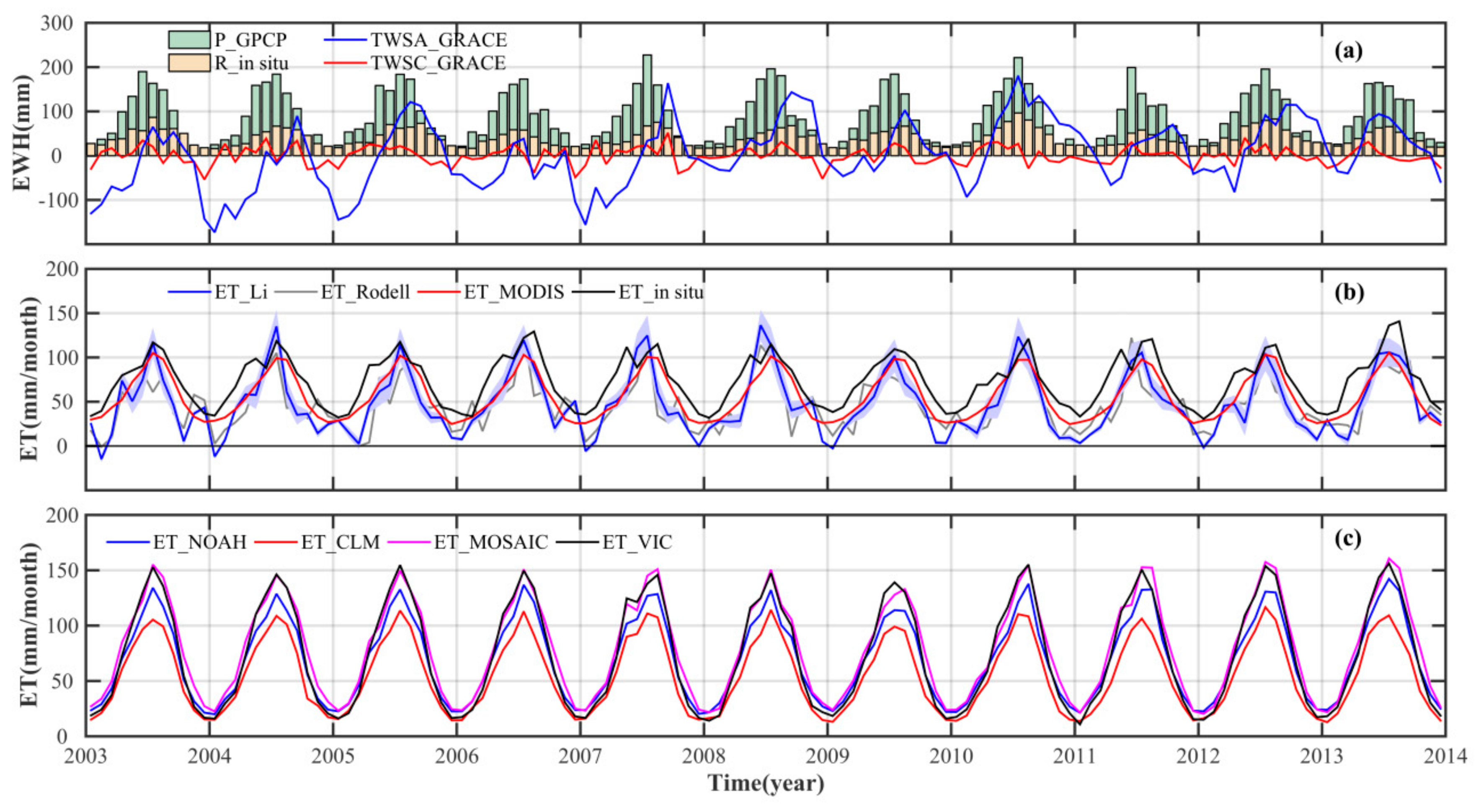
Here, the Global Precipitation Climatology Project (GPCP) One-Degree Daily (1DD) product (Version 1.2) was used to obtain the precipitation averaged over the YRB and the seven subcatchments. The GPCP product provides daily precipitation on a 1° grid over the entire globe for the period from October 1996 to the present. It is a merged analysis that incorporates precipitation estimates from both microwave-based data from the Special Sensor Microwave Imager and geosynchronous-orbit satellite infrared data, and quality-controlled surface rain gauge observations [
43]. The other daily precipitation data used were China Ground Climate daily observation Data (CGCD) (Version 3.0) (
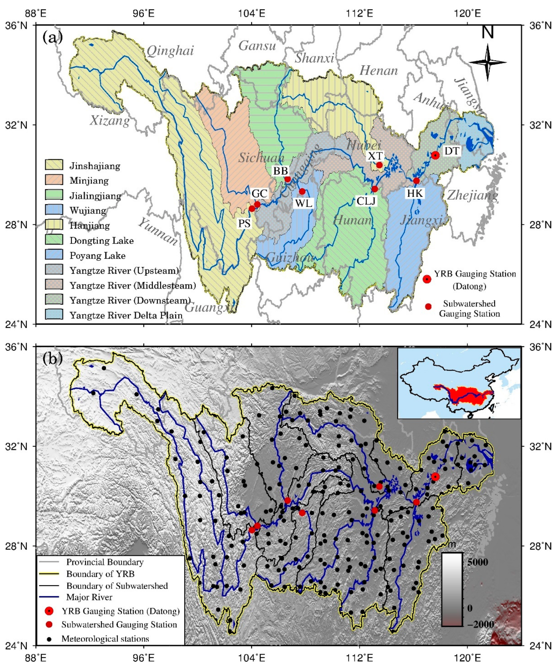
http://data.cma.cn). There are 224 meteorological stations distributed throughout the YRB that have been operational between 1951 and the present (
Figure 1b). Moreover, these meteorological stations were heterogeneously distributed over the YRB, and they were especially sparsely distributed in the northwest of YRB. Here, the daily average precipitation over the entire YRB and the seven subcatchments was estimated using a robust spatial averaging method. The monthly precipitation data of the two different products have high correlation (0.95 for the entire YRB); therefore, only the GPCP 1DD daily product was used to estimate ET in this study.
The discharge data used in this study were provided by the Changjiang Water Resources Commission of the Ministry of Water Resources. There are eight gauging stations on the upper and middle reaches of the Yangtze River (
Figure 1,
Table 1). The discharge data comprised daily observations from 2003 to 2013. We compared the mean annual values of
P from the GPCP and
R from in situ observations over the YRB with statistical observations from Changjiang and the Southwest River Water Resources Bulletin (CSWRB) (
http://www.cjw.gov.cn) for the period 2003–2013. The mean annual values of
P and
R obtained from the data used in this study were 1059.2 mm/year and 465.9 mm/year, respectively, while the mean annual values of
P and
R obtained from the CSWRB were 1044.79 mm/year and 478.75 mm/year, respectively, i.e., the values were reasonably consistent.
Three different ET products (i.e., monthly ET products from GLDAS and MODIS and daily ET products from the CGCD) were used to evaluate the GRACE-based ET in this study. The GLDAS integrates satellite data and LSM data to generate a global distribution of land surface states (e.g., ET). The ET outputs used were derived from four LSMs [
7]: Mosaic, Noah, CLM, and VIC. The MODIS-derived estimates of ET were based on the Penman–Monteith method by combining remote sensing data and meteorological observations [
5]. The monthly ET of the entire YRB and seven subcatchments were provided by the GLDAS and MODIS ET products without post-processing. The CGCD (Version 3.0) provided the daily average ET of the YRB region based on the data from the 224 meteorological stations, which observed daily ET by E-601B evaporator and small-sized evaporator. Daily ET estimates for the entire YRB and the seven subcatchments were obtained using the same spatial averaging method used for precipitation.
3.3. An Improved Approach for Estimation of Monthly ET
The hydrological water balance equation at the basin scale can be expressed as
where
P is total precipitation,
R is stream flow, ET is regional evapotranspiration over the watershed area, and
is the TWSC for a specific time period.
The daily basin-scale water balance can be written as
where
,
, and
are the daily measurements of the
ith day for
N1th month. Assuming that water storage for the beginning of the
N1th month is
, the water storage for the first day of the
N1th month could be written as
The water storage for the
ith day of the
N1th month could be written as
Rewriting Equation (6) for all days
D1 in the
N1th month and summing yields:
Then, the average water storage for the
N1th month can be written as
The second term on the right-hand side of Equation (8) is the running mean accumulation of water storage (or hydrological elements), which is not normally used in hydrology [
2]. However, the term
closely approximates the water storage observed by the GRACE satellite. Similarly, the average water storage for the
N2th month is
If
N2 =
N1 + 1, the relationship between
and
is
The difference between month
N1 and
N2 in terms of the mean monthly total TWS anomalies between months
N1 and
N2 is
Substituting Equation (10) into Equation (11), means Equation (11) becomes
Equation (12) in this study and Equation (4) in Rodell et al. [
2] are equivalent to some degree, and they could be converted into each other. Meanwhile, substituting Equation (4) into Equation (12) and taking the ET-related terms as described in Equations (14), Equation (12) can be simplified to:
The terms
and
can also be expanded as
in Equation (14). Assuming
is the total monthly ET for the
Nith month, and using
instead of the daily ET for each day in the
Nith month, Equation (14) can be rewritten as:
Many studies have estimated the total mean ET in two months (
) using Equation (13) [
2,
8,
14]. Considering Equations (13) and (15), the related terms of
P and
R can be calculated using daily precipitation and runoff observations, as mentioned in
Section 3.2, where
is the difference in TWS from GRACE in two consecutive months. Here, a set of equations related monthly ET for
N + 1 months was established, and the observation equation could be written as:
where
N + 1 is the number of monthly ET to be estimated, and the matrixes
,
,
could be expanded as
As for underdetermined system of equations, the constraint equation
was applied to obtain stable solutions, and the appropriate regularization factor
was determined using the generalized cross validation (GCV) method [
44].
The two previous methods and our method were verified by numerical simulation in our study. Firstly, the monthly GRACE-like TWS were calculated from daily
P,
R, and ET by using Equation (9). Then, taking the monthly TWS, daily
P and
R as observation data, and the ET as the unknown value, we estimated monthly ET using these three methods described above (i.e., Rodell et al. [
2], Ramillien et al. [
10] and our method). Finally, the monthly ET that converted from the daily ET, which used in the first step to calculating the monthly GRACE-like TWS, was taken as the ET true value (ET0) to verifying these three ET estimations. Including ET_Rodell, the total mean ET in two months based on the method of Rodell et al. [
2], ET_Ramillien, the results were obtained from the method of Ramillien et al. [
10] and ET_Li, and the method proposed in this study.
In order to analyze the effectiveness of the method and its feasibility in practical applications, the observation error in daily
P and
R had to be taken into account. In general, the uncertainties in daily
P and
R observations were estimated as 11% and 5%, respectively (Rodell et al. [
2,
14]).
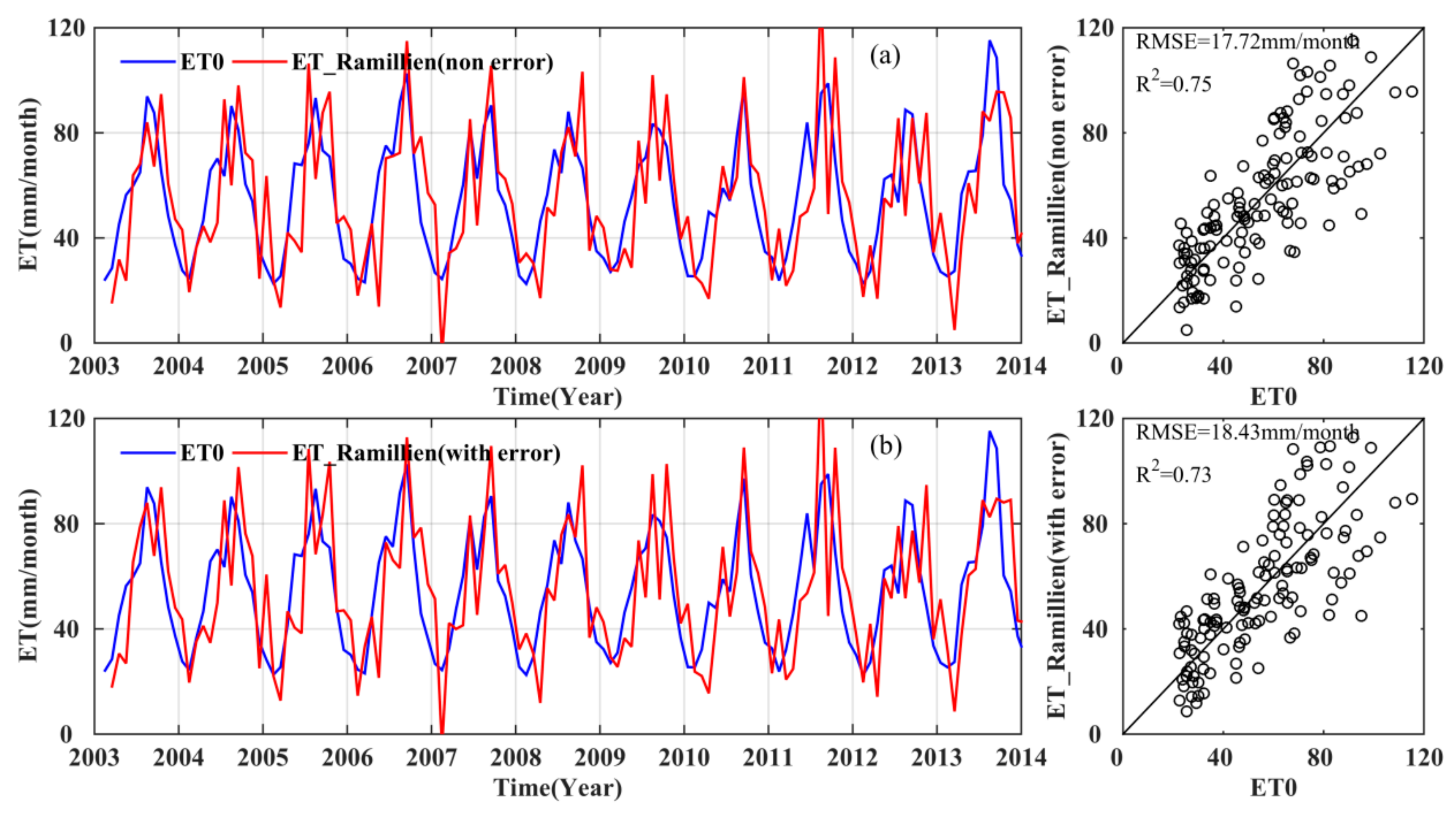
Figure 2 shows ET0 and the ET_Ramillien estimated from GRACE-like TWS and daily
P and
R without error and with observation error, using the method introduced by Ramillien et al. [
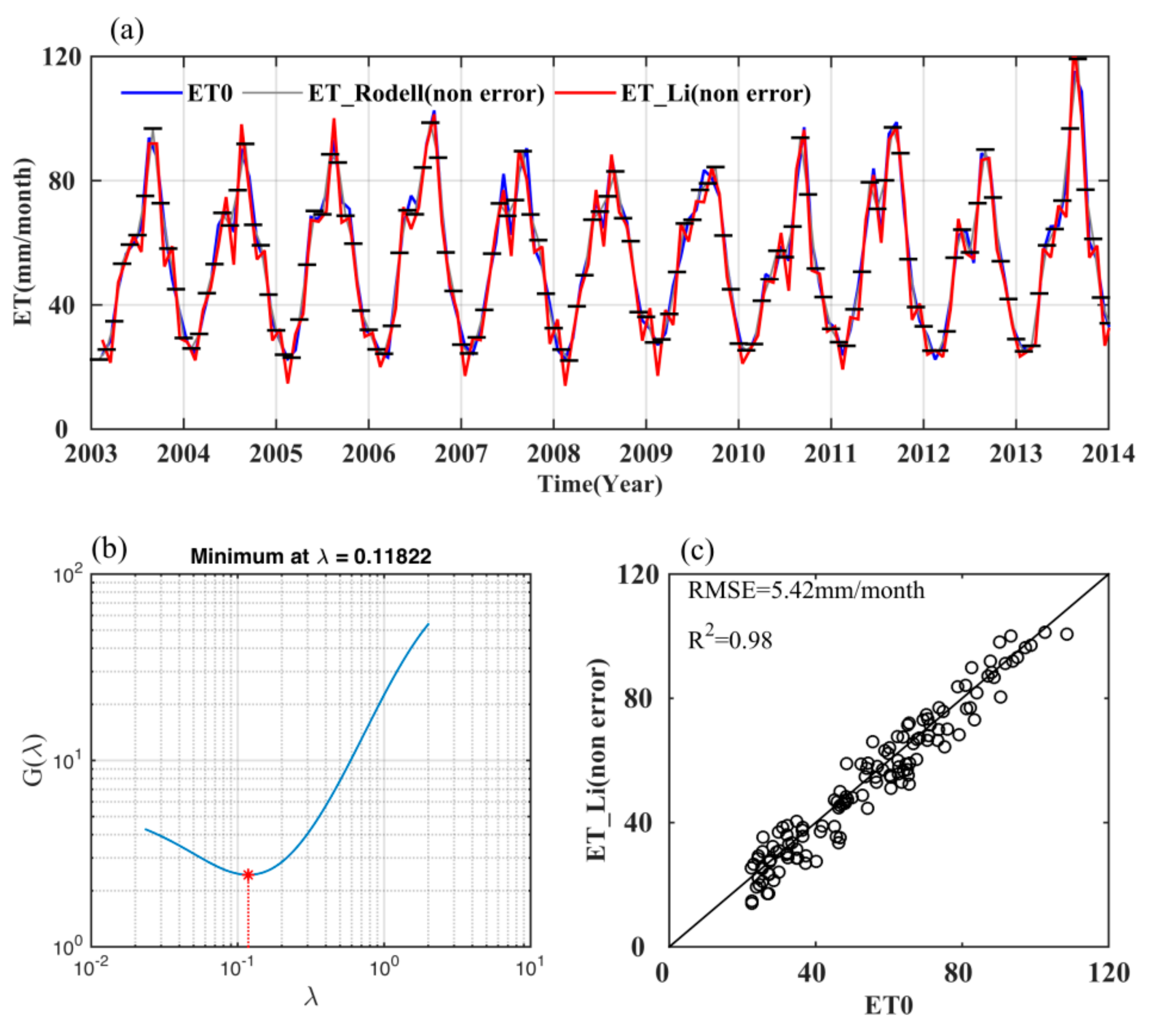
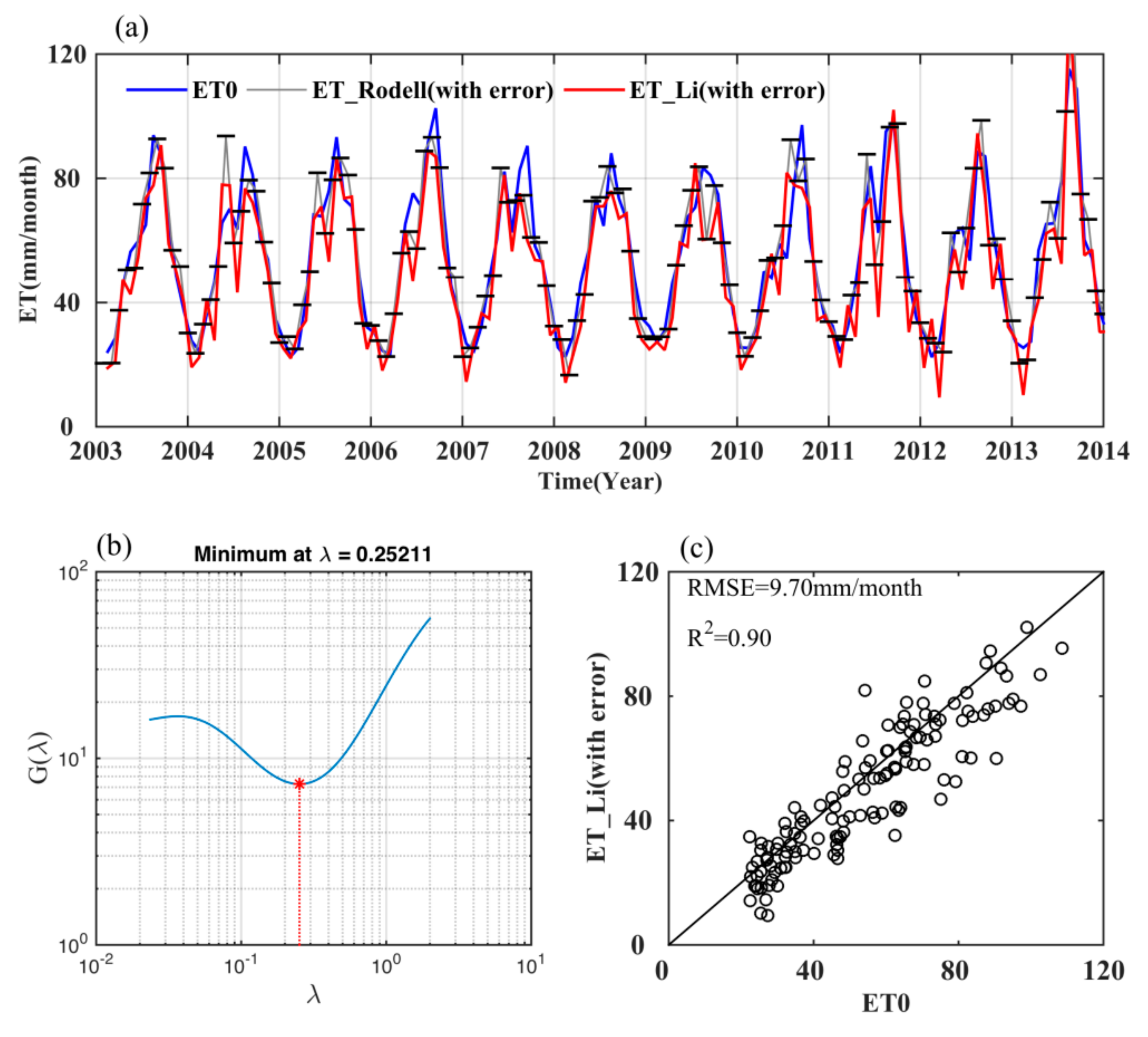
10]. Similarly,
Figure 3a and
Figure 4a show ET_Li and ET_Rodelll without and with error using the method proposed in this study and Rodell et al. [
2]. Furthermore, the regularization factors obtained from the GCV function are also shown in
Figure 3b and
Figure 4b. The estimation ET_Li and ET_Rodell in
Figure 3a are almost completely consistent with ET0, while ET_Ramillien in
Figure 2a reflects only the seasonal signal in the ET0 time series, which indicates that the ET estimation method proposed in our study and in Rodell et al. [
2] are more credible. The similar results shown in
Figure 2a,b reveal that the observation errors of daily
P and
R have little influence of the estimation of ET when using the method introduced by Ramillien et al. [
10], which both only revealing seasonal signals. The correlation coefficients (
R2) and root mean square error (RMSE) between ET0 and ET estimations were listed in
Table 2. The results showed that there is a major improvement for ET_Li relative to ET_Ramillien estimation, while comparing with ET_Rodell, ET_Li estimation has still improved to a certain degree, and the monthly ET value is isolated from ET_Rodell. In conclusion, our method can be used to estimate monthly ET efficiently. The ET results for the case study of the entire YRB discussed below were obtained using our improved approach.


