A Non-Equilibrium Sediment Transport Model for Dam Break Flow over Moveable Bed Based on Non-Uniform Rectangular Mesh

Abstract

The use of multiple-level non-uniform rectangular mesh in coupled flow and sediment transport modeling is preferred to achieve high accuracy in important region without increasing computational cost greatly. Here, a robust coupled hydrodynamic and non-equilibrium sediment transport model is developed on non-uniform rectangular mesh to simulate dam break flow over movable beds. The enhanced shallow water and sediment transport equations are adopted to consider the mass and momentum exchange between the flow phase and sediment phase. The flux at the interface is calculated by the positivity preserving central upwind scheme, which belongs to Godunov-type Riemann-problem-solver-free central schemes and is less expensive than other popular Riemann solvers while still capable of tracking wet/dry fronts accurately. The nonnegative water depth reconstruction method is used to achieve second-order accuracy in space. The model was first verified against two laboratory experiments of dam break flow over irregular fixed bed. Then the quantitative performance of the model was further investigated by comparing the computational results with measurement data of dam break flow over movable bed. The good agreements between the measurements and the numerical simulations are found for the flow depth, velocity and bed changes.

1. Introduction

Dam break flow is one of the research focuses in hydraulic engineering due to its tremendous destructive consequences. For predicting such flow the depth averaged shallow water models have been widely used in the real-life applications [1]. Early models assume the bed elevation is fixed and are only applicable to dam break flows over fixed beds [2,3,4,5,6]. However, significant sediment movements and morphological changes are commonly observed in some catastrophic flood events caused by dam failures. Therefore, it is necessary to account for the sediment transport and bed evolution when simulating dam break flow. In recent years, some numerical models have been proposed in the literature to simulate dam break flows on movable beds [7,8,9,10,11,12,13,14,15,16,17,18,19,20]. In order to improve the accuracy of simulating dam-break flow-induced sediment transport, the numerical models are evolving from equilibrium description to non-equilibrium description of sediment transport [21,22]. Equilibrium sediment transport models based on the assumption that the bed load or the total load are instantaneously adapted to equilibrium state have been widely used for morphodynamic problems [17,18,19,20]. However, the assumption of local equilibrium is not accurate for fast geomorphic transients and may lead to unrealistic results [23,24]. Compared to equilibrium models, non-equilibrium sediment transport models which take into account spatial and temporal lag effects between transport capacity and local hydrodynamic conditions are more appropriate for strong sediment transport caused by dam break flow. The main challenges in numerical aspects of developing a robust model are preserving the positivity of water depth and satisfying the well-balanced property or the C-property [25,26].

Based on the projection step, the Godunov-type schemes generally fall into two categories: upwind schemes (Riemann solver schemes) [9,12,14,17,18,19,20,27] and central schemes [6,28,29,30]. Central schemes do not require any Riemann problem solvers and characteristic decomposition, which is a powerful black-box solver for the hyperbolic partial differential equations (PDEs). Kurganov et al. [31] proposed a numerical scheme, which belongs to Godunov-type Riemann-problem-solver-free central schemes, to solve 1D and 2D shallow water equation system with discontinuous bottom topography. In order to reduce the numerical dissipation, the one-sided local speeds are adopted to estimate of the width of the Riemann fans. So the proposed central scheme has an upwind nature and is called central-upwind scheme. They proved that the central-upwind scheme is well-balanced, is able to preserve the positivity of water depth when the Courant number is less than 0.25, and has key features of the Godunov-type central schemes, i.e., robustness, efficiency and simplicity. Liu et al. [15] further shows that the central-upwind scheme is less expensive than other popular Riemann solvers while still capable of tracking wet/dry fronts accurately. The central-upwind schemes are widely used in numerical models to simulate dam break flow over fixed [6,30] and movable bed [15,21,29,32], and satisfactory simulation results are achieved. However, most of these existing models are based on uniform Cartesian grids or triangular mesh, and limited studies are dedicated to non-uniform rectangular or quadtree grids.

Uniform Cartesian grids are widely used in computational simulation of free surface flows due to it’s simplicity. However, since the same resolution has to be adopted in the whole domain, large number of computational nodes and high computational cost are needed when high-resolution grids are used. In fact, in large-scale simulations, the high-gradient regions where fine grids are required are much less than the whole computational domain [33]. In order to improve computational efficiency and at the same time maintain the required accuracy, non-uniform grids have been recently used to simulate dam break flow over movable bed, either in the form of non-uniform triangular mesh [12,15,34] or rectangular mesh [35,36]. Compared to the triangular mesh, non-uniform rectangular mesh is more convenient to achieve high order accuracy in space, while keeps most advantages of the rectangular mesh [37].

In this paper, a coupled hydrodynamic and non-equilibrium sediment transport model on non-uniform rectangular mesh is developed to simulate dam break flow over movable bed. Following Wu [1], the enhanced shallow water and sediment transport equations are adopted, including the terms that account for the mass and momentum exchange between flow phase and sediment phase. The interface flux is computed by the central-upwind scheme with second order accuracy in space. The quantitative performance of the model has been investigated by comparing the results with measurement data in four dam break laboratory experiments.

2. Governing Equations

2.1. Hydrodynamic Equations

The two-dimensional shallow water equations, which are derived by integrating the Navier-Stokes equations over depth with hydrostatic pressure assumption, are widely used to simulate dam break flow over fixed bed. However, strong sediment transport and rapid bed changes, which could generate significant effect on water flow, are occurring during dam break flow over movable beds. Thus, the enhanced shallow water equations including the mass and momentum exchange between flow phase and sediment phase to describe the hydrodynamic procedure of the dam break flow over movable bed are required, which are [1]:

$$\frac{\partial \rho h}{\partial t}+\frac{\partial \rho hu}{\partial x}+\frac{\partial \rho hv}{\partial y}=-{\rho }_b\frac{\partial z_b}{\partial t}$$

(1)

$$\frac{\partial \rho hu}{\partial t}+\frac{\partial }{\partial x}\rho (h{u}^2+\frac{1}{2}g{h}^2)+\frac{\partial \rho huv}{\partial y}=-\rho gh\frac{\partial z_b}{\partial x}-\frac{1}{2}g{h}^2\frac{\partial \rho }{\partial x}-\rho g\frac{n^{2}u\sqrt{u^2+v^2}}{h^{1/3}}$$

(2)

$$\frac{\partial \rho hv}{\partial t}+\frac{\partial \rho huv}{\partial x}+\frac{\partial }{\partial y}\rho (h{v}^2+\frac{1}{2}g{h}^2)=-\rho gh\frac{\partial z_b}{\partial y}-\frac{1}{2}g{h}^2\frac{\partial \rho }{\partial y}-\rho g\frac{n^{2}v\sqrt{u^2+v^2}}{h^{1/3}}$$

(3)

where t = time; x and y = the space coordinate; h = flow depth; u and v = flow velocity in x and y directions, respectively; $z_b$ = bed elevation; g = gravity acceleration; $\rho$ = density of water and sediment mixture; $C_t$ = the volumetric concentration of total-load sediment; ${\rho }_s$ and ${\rho }_w$ = density of sediment and water, respectively. ${\rho }_b$ = the density of the water and sediment mixture in the bed surface layer, ${\rho }_b={\rho }_{w}p+{\rho }_s(1-p)$; p = the porosity of the bed material; n = Manning’s coefficient for channel bed.

2.2. Morphodynamic Equations

Simulation of the sediment transport processes induced by dam break flow can be achieved by calculating the total-load directly [1]. Therefore, the sediment transport and bed evolution equations are given as:

$$\frac{\partial (h{C}_t)}{\partial t}+\frac{\partial (hu{C}_t)}{\partial x}+\frac{\partial (hv{C}_t)}{\partial y}=-\frac{1}{L}(\sqrt{u^2+v^2}h{C}_t-q_t)$$

(4)

$$(1-p)\frac{\partial z_b}{\partial t}=\frac{1}{L}(\sqrt{u^2+v^2}h{C}_t-q_t)$$

(5)

where $q_t$ = total-load sediment transport capacity, $q_t$ = $q_b$ + $q_s$; $q_b$ and $q_s$ = the equilibrium bed load and suspended sediment transport rate, respectively; L = the non-equilibrium adaption length.

2.3. Empirical Relations

2.3.1. Non-Equilibrium Adaptation Length

The non-equilibrium adaptation length L is a characteristic distance for sediment to adjust from a non-equilibrium state to the equilibrium state, which has been investigated by many researchers [38,39,40]. The non-equilibrium adaptation length L could be determined by [1,10]:

$$L=\max \left\{L_b,\frac{\sqrt{u^2+v^2}h}{\alpha w_s}\right\}$$

(6)

where $L_b$ = the adaptation length of bed-load, which is related to the dominant bed form or sediment transport scale; $\alpha$ = the adaptation coefficient of suspended load, whose values mostly range between 0.25 to 5.0. It should be mentioned that these two parameters are usually determined through calibration against experimental data. $w_s=w_{s0}{(1-C_t)}^m$ = settling velocity of sediment particles; m = exponent against experimental data indicating the hindered influence of high sediment concentrations on settling velocity. $w_{s0}$ = the settling velocity of a single sediment particle in quiescent water, which is given by [41]:

$$w_{s0}=\sqrt{{\left(13.95\frac{\nu }{d}\right)}^2+1.09\left(\frac{{\rho }_s}{{\rho }_w}-1\right)gd}-13.95\frac{\nu }{d}$$

(7)

where d = the diameter of the sediment particles; $\nu$ = the kinematic viscosity of water.

2.3.2. Sediment Transport Rate

The commonly-used formulas of Wu et al. [42], are adopted to calculate the equilibrium transport rate of bed load $q_b$ and suspended load $q_s$:

$$q_b=0.0053\sqrt{\left(\frac{{\rho }_s}{{\rho }_w}-1\right)g{d}^3}{\left[\frac{{\tau }_{be}}{{\tau }_{cr}}-1\right]}^{2.2}$$

(8)

$$q_s=0.0000262\sqrt{\left(\frac{{\rho }_s}{{\rho }_w}-1\right)g{d}^3}{\left[\left(\frac{{\tau }_b}{{\tau }_{cr}}-1\right)\frac{\sqrt{u^2+v^2}}{w_s}\right]}^{1.74}$$

(9)

where ${\tau }_{be}$ = effective bed shear stress, ${\tau }_{be}={(n^{\prime }/n)}^{3/2}{\tau }_b$; $n^{\prime }$ = Manning’s coefficient related to grain roughness, $n^{\prime }=d^{1/6/}20$; n = Manning’s coefficient for channel bed; ${\tau }_b$ = bed shear stress, ${\tau }_b=g{n}^2(u^2+v^2)({\rho }_s-{\rho }_w)gd/h^{1/3}$; ${\tau }_c$ = the critical bed shear stress for incipient sediment motion, which is calculated using the relationship of Wu et al. [42]:

$${\tau }_c=0.03({\rho }_s-{\rho }_w)gd$$

(10)

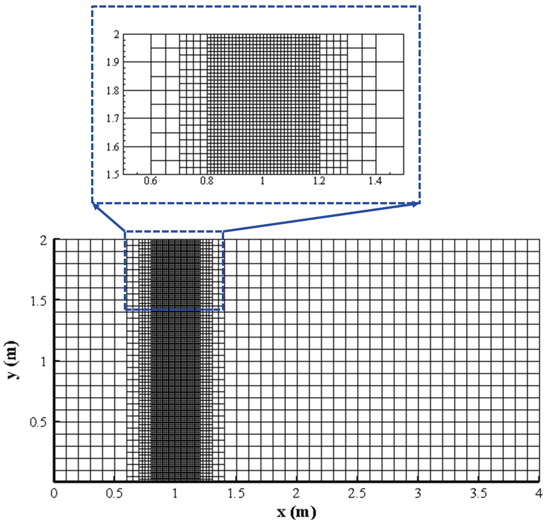
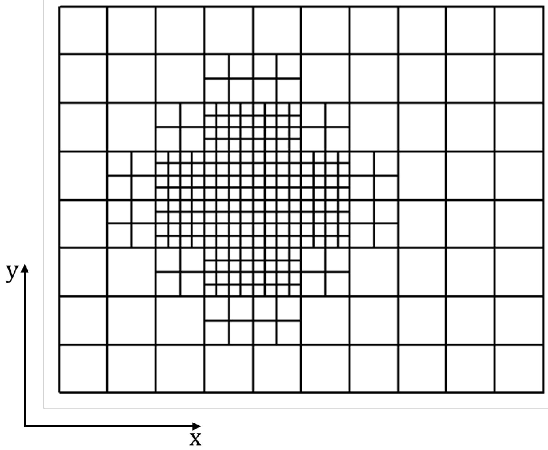
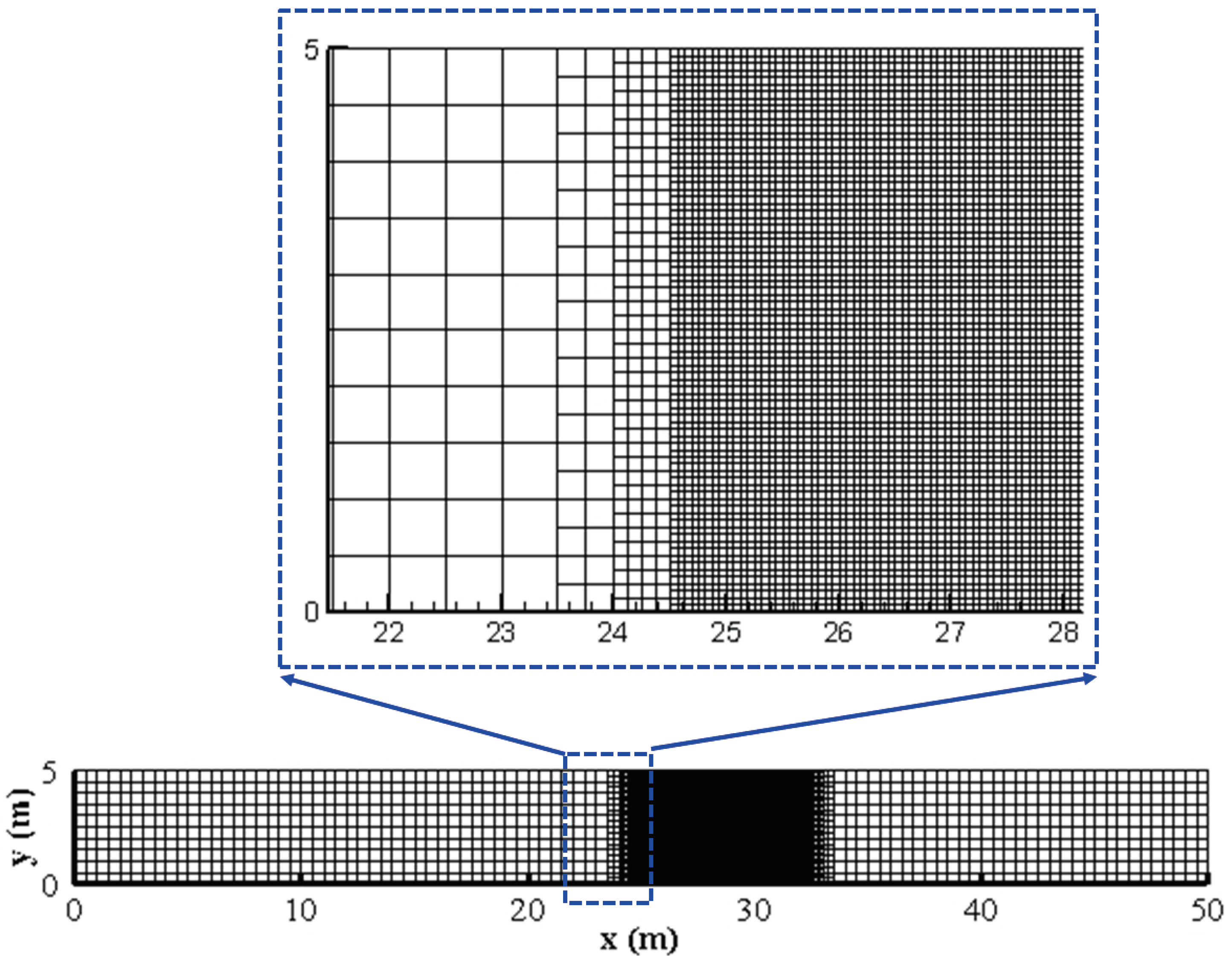
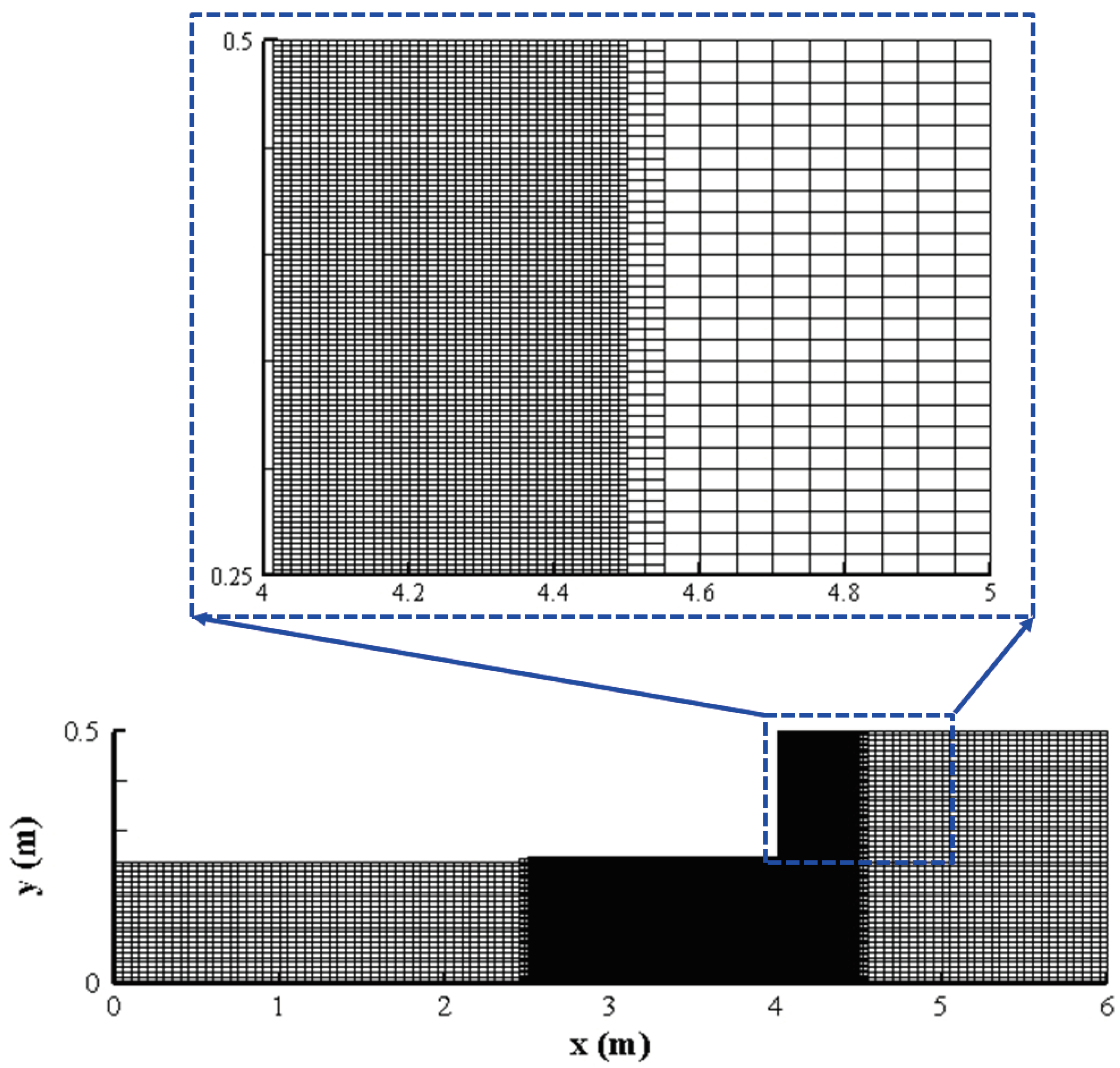
2.4. Non-Uniform Rectangular Mesh

The non-uniform rectangular mesh, as shown in Figure 1, is used in this study. To obtain this non-uniform rectangular mesh, a straightforward method proposed by Liang [33] is implemented: Firstly, the whole computational domain is discretized by a coarse uniform rectangular grid. Then, a specific subdivision level is allocated to the coarse background cell and the coarse cell will be divided into $2^{lev}\times 2^{lev}$ fine elements, where $lev$ = a subdivision level. Finally, regularize the grid to make sure that any cell is at most two times bigger or smaller than its neighbors (2:1 rule), as shown in Figure 1. After regularization of the grid, neighboring cells for an arbitrary cell could be determined by a simple algebraic relationship [33]. Moreover, in order to simplify the computer programing and reduce memory usage, the computational cells are numbered in a 1D sequence and a non-staggered approach is used, which defines all primary variables h, u, v, and $C_t$ at cell centers and represent the average values of each cell.

3. Numerical Method

In this study, a central upwind scheme based on finite volume method is used to solve the equations for the dam break flow problem, which involves mix flow regimes and sediment transport. Second-order accuracy in space is achieved by the nonnegative water depth reconstruction method proposed by Liang [4]. More details of the numerical method is given in the following paragraphs. In order to present this numerical method clearly and compactly, Equations (1)–(4) is reformulated into a shallow water equation system and written in vector form:

$$\frac{\partial \mathbf{Q}}{\partial t}+\frac{\partial \mathbf{F}}{\partial x}+\frac{\partial \mathbf{G}}{\partial y}=\mathbf{S}$$

(11)

$$\mathbf{Q}=\left[\begin{array}{c}\eta \\ hu\\ hv\\ h{C}_t\end{array}\right]\mathbf{F}=\left[\begin{array}{c}hu\\ h{u}^2+\frac{1}{2}g{h}^2\\ huv\\ hu{C}_t\end{array}\right]\mathbf{G}=\left[\begin{array}{c}hv\\ huv\\ h{v}^2+\frac{1}{2}g{h}^2\\ hv{C}_t\end{array}\right]$$

$$\mathbf{S}=\left[\begin{array}{c}0\\ -gh\frac{\partial z_b}{\partial x}-\frac{gu\sqrt{u^2+v^2}{n}^2}{h^{1/3}}-\frac{1}{2\rho }g{h}^2\frac{\partial \rho }{\partial x}+u\frac{{\rho }_s-{\rho }_w}{\rho }(1-\frac{C_t}{1-p})\frac{\sqrt{u^2+v^2}h{C}_t-q_t}{L}\\ -gh\frac{\partial z_b}{\partial y}-\frac{gv\sqrt{u^2+v^2}{n}^2}{h^{1/3}}-\frac{1}{2\rho }g{h}^2\frac{\partial \rho }{\partial y}+v\frac{{\rho }_s-{\rho }_w}{\rho }(1-\frac{C_t}{1-p})\frac{\sqrt{u^2+v^2}h{C}_t-q_t}{L}\\ \frac{1}{1-p}\frac{\sqrt{u^2+v^2}h{C}_t-q_t}{L}\end{array}\right]$$

where $\eta$ = water surface elevation, $\eta =h+z_b$. $\mathbf{Q}$ = a vector of the conserved variables. $\mathbf{F}$ and $\mathbf{G}$ = the flux vectors in x and y direction, respectively. $\mathbf{S}$ = the source term vectors which include bed slope terms and bed friction terms.

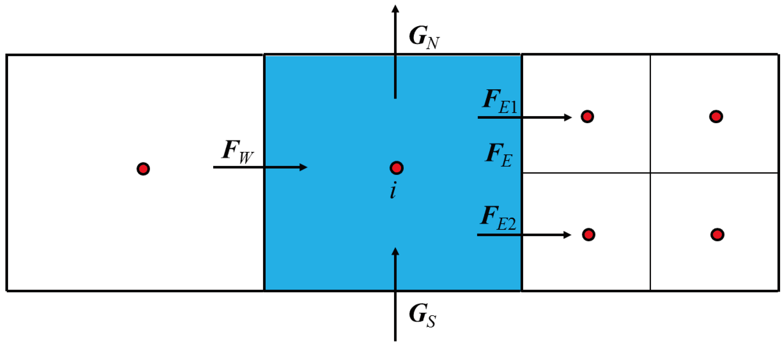
3.1. Finite Volume Discretization

Integrating of Equation (11) over non-uniform rectangular control element i shown in Figure 2, and applying the Green theorem and the Euler time-integration method, one can get the following discretized equation:

$${\mathbf{Q}}_i^{o+1}={\mathbf{Q}}_i^o-\frac{\Delta t}{\Delta x}({\mathbf{F}}_E-{\mathbf{F}}_W)-\frac{\Delta t}{\Delta y}({\mathbf{G}}_N-{\mathbf{G}}_S)+\Delta t{\mathbf{S}}_i$$

(12)

where the superscript o = the time level and subscript i = the index of the cell. $\Delta t$ = the time step. $\Delta x$ and $\Delta y$ = cell sizes in x and y directions, respectively. ${\mathbf{F}}_E$, ${\mathbf{F}}_W$, ${\mathbf{G}}_N$ and ${\mathbf{G}}_S$ = the fluxes through the east, west, north and south cell interfaces, respectively. ${\mathbf{S}}_i$ = the source term at the cell center.

It should be mentioned that when evaluating the flux through the interface of two cells with different sizes, special attention must be taken to maintain the mass and momentum conservation. As shown in Figure 2, two smaller rectangular cells locate at the right side of the cell i. The flux vector ${\mathbf{F}}_E$ through the eastern interface could not be directly calculated, but given by ${\mathbf{F}}_E=({\mathbf{F}}_{E1}+{\mathbf{F}}_{E2})/2$, where ${\mathbf{F}}_{E1}$ and ${\mathbf{F}}_{E2}$ are the fluxes through the western interface of two smaller neighboring cells. This step could preserve the conservative property of the finite volume scheme.

3.2. Nonnegative Water Depth Reconstruction

To ensure the C-property and deal with wetting and drying accurately in a uniform rectangular grid Liang [4] proposed a nonnegative water depth reconstruction method. In this section the same procedure has been extended in 2D non-uniform rectangular grids to achieve second order accuracy in space and C-property.

Firstly, the Riemann states, the conserved variables ($\eta$, $hu$, $hv$) and water depth h at interface, are reconstructed from the available flow information at the cell center. For a cell i the left Riemann states at the cell interface $i+1/2$ in x direction (eastern face) are given by:

$${\overline{\eta }}_{i+1/2,x}^L={\eta }_i+\frac{1}{2}{\phi }_i({\eta }_i-{\eta }_{i-1,x})$$

(13)

$${\overline{h}}_{i+1/2,x}^L=h_i+\frac{1}{2}{\phi }_i(h_i-h_{i-1,x})$$

(14)

$${\overline{uh}}_{i+1/2,x}^L=u{h}_i+\frac{1}{2}{\phi }_i(u{h}_i-u{h}_{i-1,x})$$

(15)

$${\overline{vh}}_{i+1/2,x}^L=v{h}_i+\frac{1}{2}{\phi }_i(v{h}_i-v{h}_{i-1,x})$$

(16)

where ${\phi }_i$ = a slope limiter evaluated separately for considered variables. In this study the minmod limiter is used. The velocity components of interface are calculated as:

$${\overline{u}}_{i+1/2,x}^L=\frac{{\overline{uh}}_{i+1/2,x}^L}{{\overline{h}}_{i+1/2}},{\overline{v}}_{i+1/2,x}^L=\frac{{\overline{vh}}_{i+1/2,x}^L}{{\overline{h}}_{i+1/2}}$$

(17)

When the cell is dry ($h<{10}^{-8}$ m), the velocities are set to be zero and not calculated by Equation (17). The left bed elevation at the cell interface $i+1/2$ in x direction is given by

$${(\overline{z_b})}_{i+1/2,x}^L={\overline{\eta }}_{i+1/2,x}^L-{\overline{h}}_{i+1/2,x}^L$$

(18)

The right Riemann states ${\overline{\eta }}_{i+1/2,x}^R$, ${\overline{h}}_{i+1/2,x}^R$, ${\overline{uh}}_{i+1/2,x}^R$, ${\overline{vh}}_{i+1/2,x}^R$, ${\overline{u}}_{i+1/2,x}^R$, ${\overline{v}}_{i+1/2,x}^R$ and ${(\overline{z_b})}_{i+1/2,x}^R$ at the cell interface $i+1/2$ in x direction can be obtained using the similar method. Then, a single value of bed elevation at the cell interface $i+1/2$ is defined following Audusse et al. [43]:

$${(z_b)}_{i+1/2,x}=\max \left\{{(\overline{z_b})}_{i+1/2,x}^L,{(\overline{z_b})}_{i+1/2,x}^R\right\}$$

(19)

In order to preserve the reconstructed water depth to be nonnegative, the face values of water depth are corrected as:

$$\begin{array}{c}{h}_{i+1/2,x}^L=\max \left\{0,{\overline{\eta }}_{i+1/2,x}^L-{(z_b)}_{i+1/2,x}\right\}\hfill \\ h_{i+1/2,x}^R=\max \left\{0,{\overline{\eta }}_{i+1/2,x}^R-{(z_b)}_{i+1/2,x}\right\}\hfill \end{array}$$

(20)

Finally, the rest Riemann states can be recalculated by:

$${\eta }_{i+1/2,x}^L=h_{i+1/2,x}^L+{(z_b)}_{i+1/2,x}$$

(21)

$${uh}_{i+1/2,x}^L={\overline{u}}_{i+1/2,x}^L{h}_{i+1/2,x}^L$$

(22)

$${vh}_{i+1/2,x}^L={\overline{v}}_{i+1/2,x}^L{h}_{i+1/2,x}^L$$

(23)

$${\eta }_{i+1/2,x}^R=h_{i+1/2,x}^R+{(z_b)}_{i+1/2,x}$$

(24)

$${uh}_{i+1/2,x}^R={\overline{u}}_{i+1/2,x}^R{h}_{i+1/2,x}^R$$

(25)

$${vh}_{i+1/2,x}^R={\overline{v}}_{i+1/2,x}^R{h}_{i+1/2,x}^R$$

(26)

In general the above reconstruction procedure will not affect the C-property of the numerical scheme. However, further modifications need to be implemented if the bed elevation of the dry cell is higher than the water surface elevation of the neighbor wet cell [4]:

$$\Delta z=\max \left\{0,{(z_b)}_{i+1/2,x}-{\eta }_{i+1/2,x}^L,{(z_b)}_{i+1/2,x}-{\eta }_{i+1/2,x}^R\right\}$$

(27)

$$\begin{array}{cc}\hfill {(z_b)}_{i+1/2,x}& \leftarrow {(z_b)}_{i+1/2,x}-\Delta z\hfill \\ \hfill {\eta }_{i+1/2,x}^L& \leftarrow {\eta }_{i+1/2,x}^L-\Delta z\hfill \\ \hfill {\eta }_{i+1/2,x}^R& \leftarrow {\eta }_{i+1/2,x}^R-\Delta z\hfill \end{array}$$

(28)

This treatment makes the reconstructed bed elevation equal to water level at the interface of the wet cell and the dry cell, which ensures the numerical scheme to be well balanced for the dry-bed application.

3.3. Numerical Fluxes Calculation

The central-upwind scheme proposed by Kurganov et al. [31] is applied to calculate mass and momentum flux (the first three components of $\mathbf{F}$ and $\mathbf{G}$) at interface. Taking the calculation of flux through the cell interface $i+1/2$ in x direction as an example, the mass and momentum flux can be calculated as:

$$\begin{array}{cc}\hfill {\mathbf{F}}_{i+1/2,x}(1:3)=& \frac{a_{i+1/2,x}^{+}\mathbf{F}({\mathbf{Q}}_{i+1/2,x}^L)-a_{i+1/2,x}^{-}\mathbf{F}({\mathbf{Q}}_{i+1/2,x}^R)}{a_{i+1/2,x}^{+}-a_{i+1/2,x}^{-}}\hfill \\ & +\frac{a_{i+1/2,x}^{+}{a}_{i+1/2,x}^{-}}{a_{i+1/2,x}^{+}-a_{i+1/2,x}^{-}}({\mathbf{Q}}_{i+1/2,x}^R-{\mathbf{Q}}_{i+1/2,x}^L)\hfill \end{array}$$

(29)

where ${\mathbf{Q}}_{i+1/2,x}^L$ and ${\mathbf{Q}}_{i+1/2,x}^R$ = the reconstructed Riemann states on the left and right side of the cell interface $i+1/2$ in x direction, respectively. $a_{i+1/2,x}^{+}$ and $a_{i+1/2,x}^{+}$ = one-sided local wave speeds on the left and right side of the cell interface $i+1/2$ in x direction, respectively and are calculated by:

$$a_{i+1/2,x}^{+}=\max \left\{u_{i+1/2,x}^L+\sqrt{g{h}_{i+1/2,x}^L},u_{i+1/2,x}^R+\sqrt{g{h}_{i+1/2,x}^R},0\right\}$$

(30)

$$a_{i+1/2,x}^{-}=\max \left\{u_{i+1/2,x}^L-\sqrt{g{h}_{i+1/2,x}^L},u_{i+1/2,x}^R-\sqrt{g{h}_{i+1/2,x}^R},0\right\}$$

(31)

The sediment transport flux (the fourth component of $\mathbf{F}$ and $\mathbf{G}$) at interface is determined by upwind scheme. Thus, the sediment flux can be calculated as:

$$\begin{array}{cc}\hfill {\mathbf{F}}_{i+1/2,x}(4)=& \max \left\{{\mathbf{F}}_{i+1/2,x}(1),0.0\right\}{(C_t)}_{i+1/2,x}^L\hfill \\ & +\min \left\{{\mathbf{F}}_{i+1/2,x}(1),0.0\right\}{(C_t)}_{i+1/2,x}^R\hfill \end{array}$$

(32)

where ${(C_t)}_{i+1/2,x}^L$ and ${(C_t)}_{i+1/2,x}^R$ = the volumetric sediment concentration in cells located on the left and right hand sides of interface $i+1/2$ in x direction, respectively. ${\mathbf{F}}_{i+1/2,x}(1)$ = mass flux calculated by Equation (29).

3.4. Treatment of Bed Slope and Friction Source Terms

The bed slope source terms are simply evaluated by central difference method and no special treatments are needed to ensure the well balance property. Taking the bed-slope source term in x direction as an example:

$$-gh\frac{\partial z_b}{\partial x}=-g\frac{h_{i+1/2,x}^L+h_{i-1/2,x}^R}{2}\frac{{(z_b)}_{i+1/2,x}-{(z_b)}_{i-1/2,x}}{\Delta x}$$

(33)

Similarly, the bed slope term for y direction can be discretized using the same method.

Since the water depth is present in the denominator of the friction source term, the fully explicit scheme for friction term may lead to instability of the numerical scheme when the water depth becomes very small. Therefore, the semi-implicit scheme, which is more stable than explicit scheme, is used to discretize the friction term:

$$\frac{g\sqrt{u^2+v^2}{n}^2}{h^{1/3}}(u,v)={\left(\frac{g\sqrt{u^2+v^2}{n}^2}{h^{4/3}}\right)}_i^o({hu}_i^{o+1},{hv}_i^{o+1})$$

(34)

3.5. Bed Deformation Calculation

The bed deformation is updated at each time step using the following explicit equation:

$${(z_b)}_i^{o+1}={(z_b)}_i^o+\frac{\Delta t}{1-p}\frac{{(\sqrt{u^2+v^2}h{C}_t-q_t)}_i^o}{L}$$

(35)

3.6. Model Stability

The above numerical model is explicit and its stability is controlled by the Courant-Friedrichs-Lewy (CFL) condition. Therefore, the time step can be expressed as:

$$\Delta t=Cr\min \left\{\frac{\Delta x}{\left|u\right|+\sqrt{(gh)}},\frac{\Delta y}{\left|v\right|+\sqrt{(gh)}}\right\}$$

(36)

where $Cr$ = the Courant number specified in the range $0<Cr<0.25$ and $Cr=0.2$ is adopted in all simulations in this study.

4. Model Validation

In this section, four laboratory experiments are used to test the performance of the proposed model. The first two cases are adopted to test the capability of the developed model to simulate dam break flow over fixed irregular bed with wetting and drying. Then, the model is validated against two benchmark tests of dam break flow over a dry and erodible bed to demonstrate it can simulate sediment transport and bed erosion with reasonable accuracy. For all tests, g = 9.8 m/s² and ${\rho }_w$ = 1000 kg/m³.

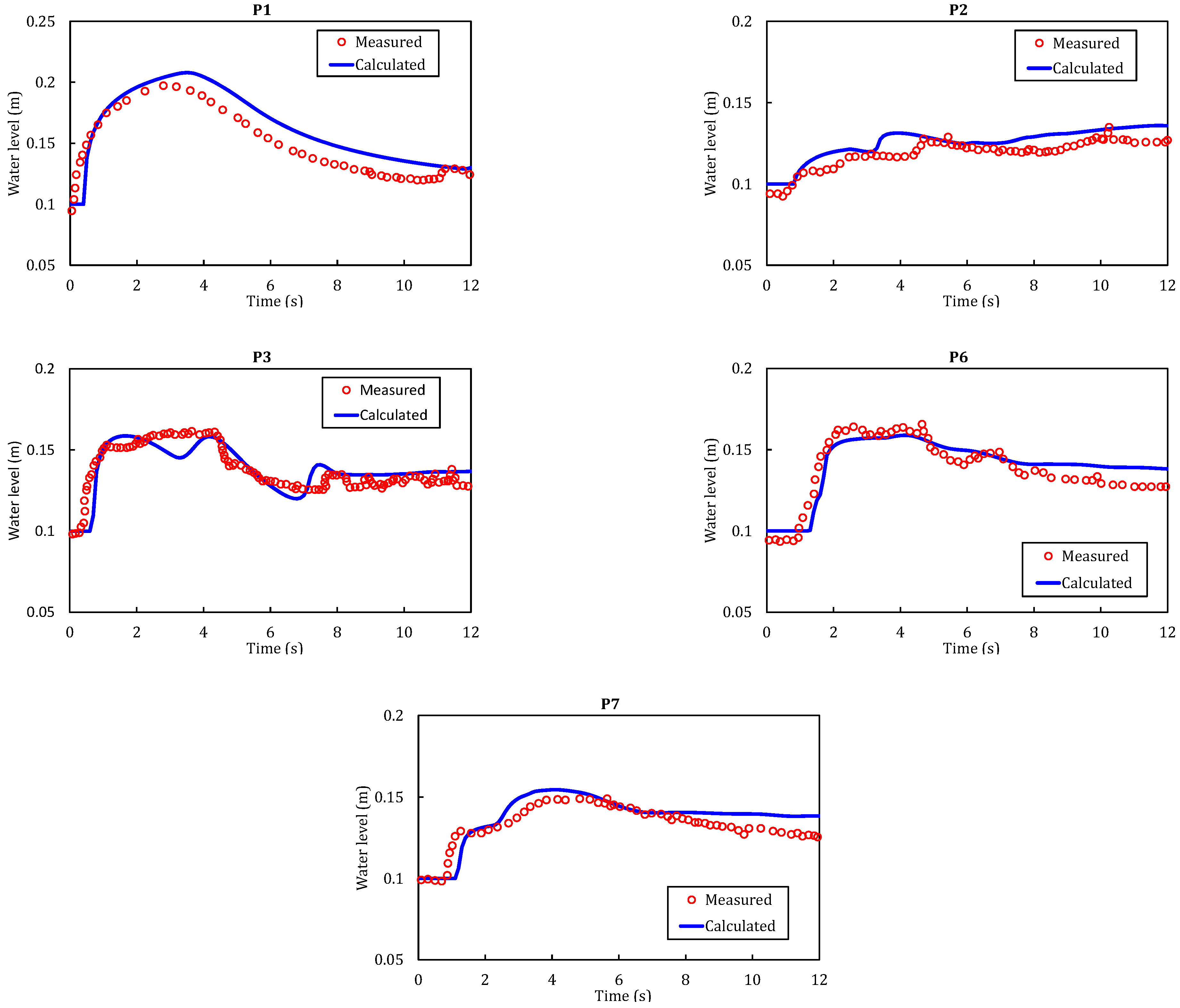
4.1. Partial Dam Break Experiment

The partial dam break experiment conducted by Fraccarollo and Toro [2] is used to evaluate the accuracy of the numerical model to simulate dam break flow over a fixed flat bed with wetting and drying. The detailed setup of the experiment is shown in Figure 3, in which the whole domain is 4 m long and 2 m wide. The dam with a breach of 0.4 m is located 1 m away from the upstream end. The initial water surface elevation in the reservoir surrounded by solid walls is 0.6 m, while the downstream flood plain is initially dry and has open boundaries in three sides. The breach in the middle of the dam is removed instantaneously at t = 0 s and the water in the reservoir rushes onto the downstream flood plain. Five gauges are placed at different locations to record the time history of water depth. The coordinates of five gauges are given in

Table 1. Coordinates of gauge stations.

Stations	5A	C	4	0	8A
x/m	0.18	0.48	1.00	1.00	1.72
y/m	1.00	0.40	1.16	1.00	1.00

.

In this simulation, the computational domain is firstly discretized by 40 × 20 rectangular cells with a uniform cell size of 0.1 m. The area near the breach with high water surface gradient is subdivided and the subdivision level is set to be 3. Figure 4 presents the non-uniform rectangular grids for the whole domain. The total simulation time is 10 s and the time step is adaptively determined by the CFL condition. Figure 5 presents the comparisons between the calculated and measured time history of water depth at five gauge stations. It can be found that the numerical water depth agree quite well with the measured data, which demonstrate that the model is able to simulate dam break flow over fixed flat bed with wetting and drying accurately.

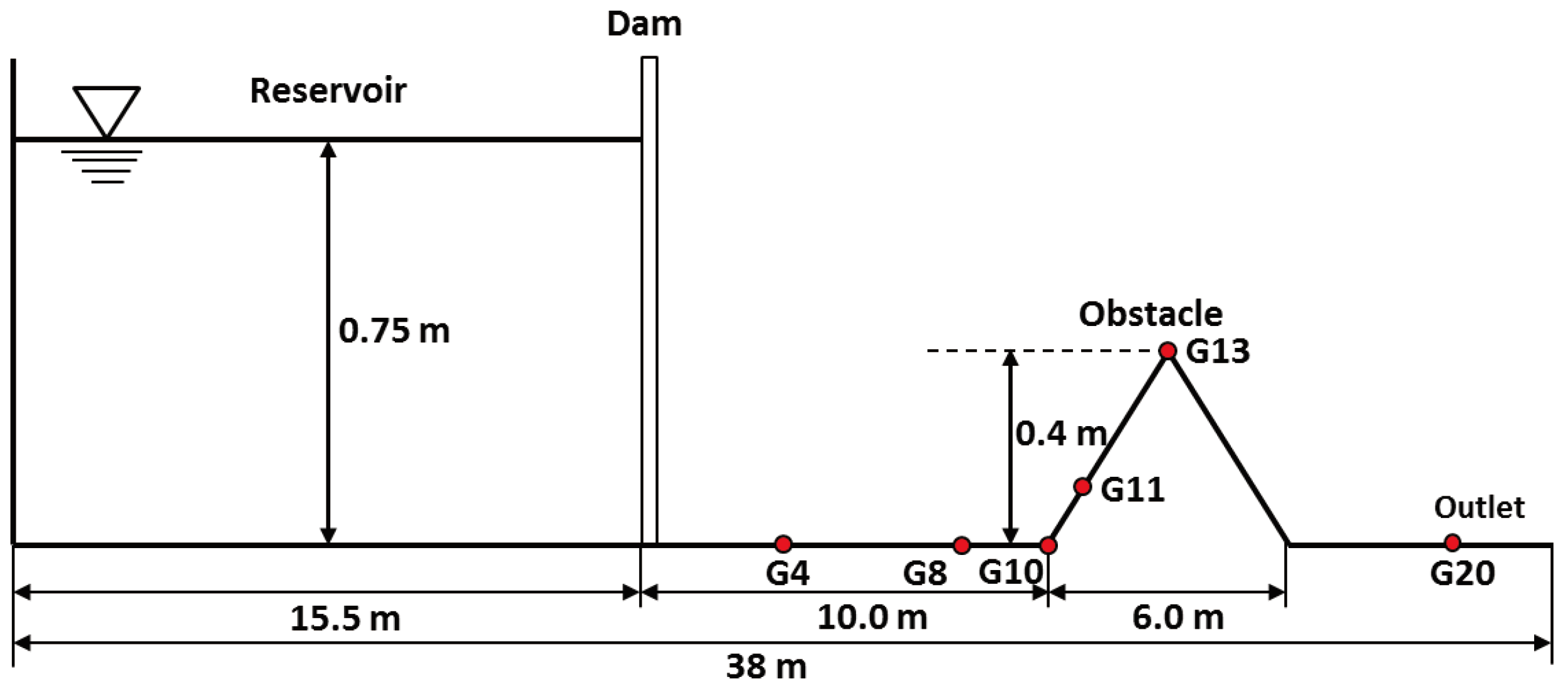
4.2. Simulation of Dam Break Flow over Triangular Obstacle

The laboratory experiment of dam break flow over triangular obstacle, which was performed in the Concerted Action on Dam-Break Modeling (CADAM) project [44] and had been widely used as an benchmark test by many researchers [14,21,36,45] , is considered to validate the current model’s ability to simulate dam break flow with wet/dry front over fixed irregular bed. Figure 6 presents the configuration of the experiment, in which the flume is 38 m long and the dam is located 15.5 m away from the upstream end. A symmetric triangular obstacle of 0.4 m high and 6 m long is installed at 13 m downstream of the dam. The initial water level in the reservoir is 0.75 m and the downstream area is a dry bed. The dam suddenly fails at t = 0 s and the water in the reservoir flows to the downstream area. As shown in Figure 6, six gauges are located at 4 m(G4), 8 m(G8), 10 m(G10), 11 m(G11), 13 m(G13) and 20 m(G20) away from dam to record the time history of water depth. The boundary conditions for the upstream and downstream ends are solid wall and free outlet, respectively.

Figure 7 presents the computational grid for decomposing the whole domain, in which the cell size of the background grid is 0.5 m and subdivision level 3 is applied to the triangular obstacle. As suggested by Liang and Marche [45], the Manning’s coefficient is set to be 0.0125. The simulation is run for 90 s. Figure 8 shows the calculated time history of water depth at six gauges. It can be seen the water depths and arrival time of the wave are well predicted except for gauge G20. Compared to the measurement data, the water depth is overestimated by the present model and the similar discrepancy was also presented in other models [45,46,47], which used different numerical schemes. One possible explanation for this deviation is the depth integrated governing equations is not suitable for the complex water flow phenomenon between triangular obstacle and outlet. In order to further evaluate the differences between the calculated and measured water depths quantitatively, the average discrepancy ($L_1$ norm) is defined as $L_1={\displaystyle \sum _{n=1}^N}|{\Lambda }_n^{mea}-{\Lambda }_n^{sim}|/N$, where ${\Lambda }_n^{mea}$ = the nth measurement data, ${\Lambda }_n^{sim}$ = the simulated result for the corresponding variables, N = the total number of the measurement data. The average discrepancies $L_1$ of water depth for six gauges are 0.018 m(G4), 0.019 m(G8), 0.032 m(G10), 0.03 m(G11), 0.008 m(G13) and 0.024 m(G20), respectively. Overall, the calculated result agree with measurements quite well and the wet/dry fronts are well captured, which confirms the effectiveness and robustness of our model to deal with dam break flow over fixed irregular bed with wet/dry fronts.

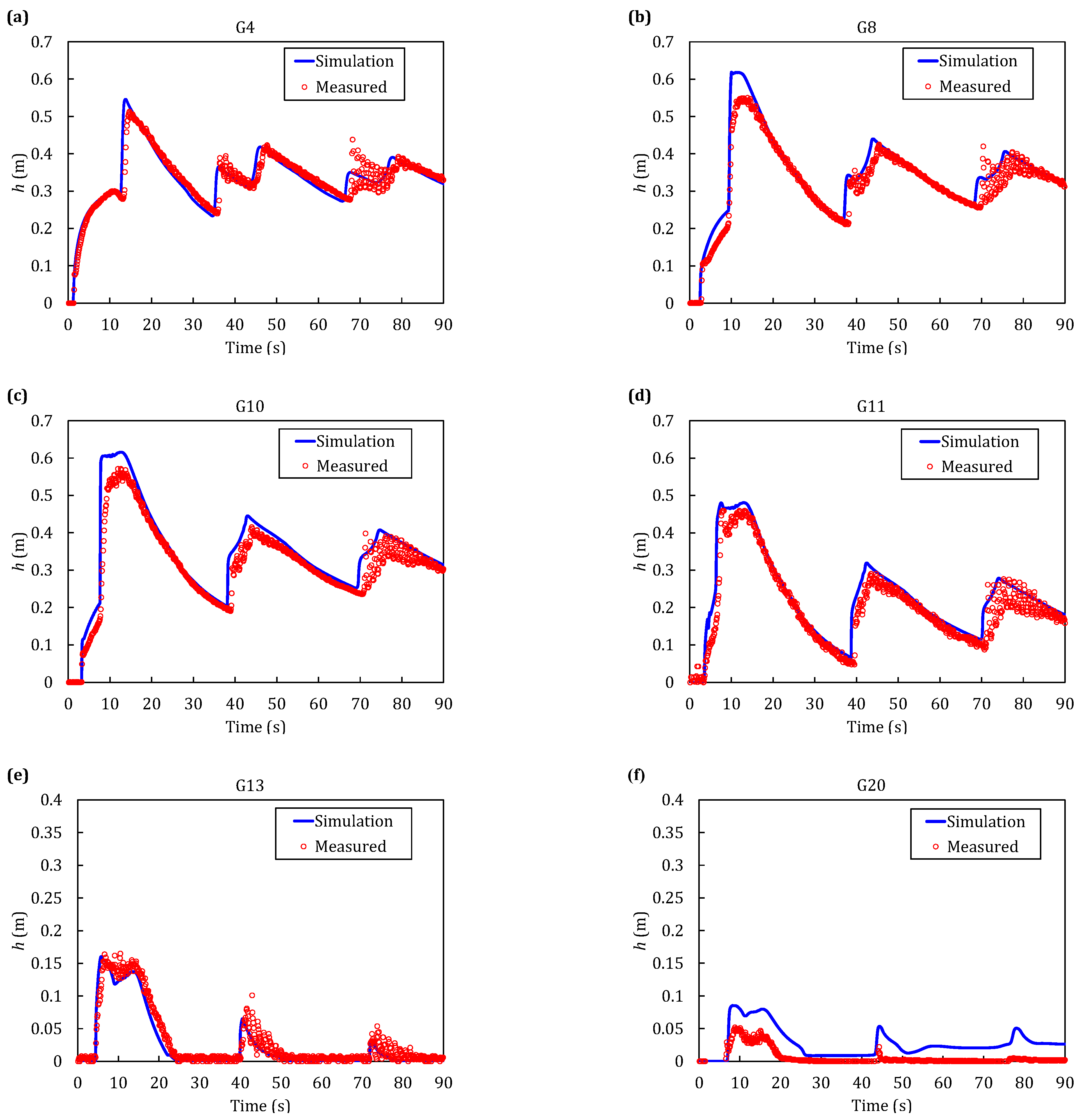
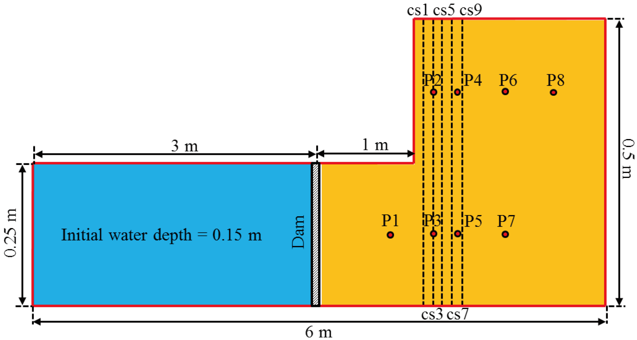
4.3. Dam-Break Flow in an Erodible Channel with a Sudden Enlargement

In order to validate the ability of the present model to deal with dam-break flow over movable bed, an experiment of dam-break flow in an erodible channel with a sudden enlargement conducted in the laboratory of Université catholique de Louvain (UCL) in Belgium [48,49] , which had been used by many researchers [14,17,18,19,22,27] to test their models, is simulated here. As shown in Figure 9, the experimental flume is 6 m long with a sudden enlargement of width from 0.25 m to 0.5 m at 4 m downstream of the inlet. The whole flume is covered by a layer of 0.1 m thick, fully saturated sand with a median diameter of 1.82 mm. The density of the sand is 2680 kg/m³, and the deposit porosity is 0.47. The dam is installed at 1 m upstream of the sudden expansion and the initial water depth in the upstream and downstream of the dam are 0.25 m and 0 m, respectively. Eight ultrasonic gauges P1–P8 are placed at downstream of channel to record the water level in a period of 12 s, and the coordinates of gauges are given in

Table 2. Coordinates of ultrasonic gauges for experiment of dam-break flow in an erodible channel with a sudden enlargement.

Gauges	P1	P2	P3	P4	P5	P6	P7	P8
x/m	0.75	1.20	1.20	1.45	1.45	1.95	1.95	2.45
y/m	0.00	0.25	0.00	0.25	0.00	0.25	0.00	0.25

. At the end of the experiment, the bed elevations at nine cross sections cs1–cs9 located every 5 cm from 10 to 50 cm after the sudden expansion are measured using a laser sheet imaging technique.

For the simulation, the computational domain is firstly discretized by coarse rectangular grids with dimension of 0.05 m × 0.01 m. Then, the area located between 2.5 m and 4.5 m away from upstream end is refined and the subdivision level is set to be 2. Figure 10 presents the computational grids for the whole domain. As suggested by Wu et al. [27], the calibrated suspended-load adaptation coefficient $\alpha$ is equal to 4.0, the adaptation length of bed-load $L_b$ is set to be 0.025 m, and the Manning’s coefficient is given as 0.025.

Figure 11 shows the calculated and measured water level at gauges P1, P2, P3, P6 and P7 in a period of 12 s. It can be found that the calculated water level agree with the measurement data quite well. The average discrepancies $L_1$ of water level at five gauges (i.e., P1, P2, P3, P6 and P7) are 0.0130 m, 0.0064 m, 0.0068 m, 0.0066 m and 0.0064 m, respectively. Figure 12 presents the comparison of the calculated and measured bed elevation at five cross sections: cs1, cs3, cs5, cs7 and cs9. At cross sections cs1 and cs3, the deposition height along the left side of the channel is underestimated, but the general erosion and deposition patterns are reproduced. At cross sections cs5, cs7 and cs9, the calculated bed elevation profiles are in good agreements with measured values. The average discrepancies $L_1$ of bed elevation at five cross sections (i.e., cs1, cs3, cs5, cs7 and cs9) are 0.0075 m, 0.0067 m, 0.0052 m, 0.0039 m and 0.0028 m, respectively. Figure 12 also shows the calculated bed profile by Juez et al. [18] and Wu et al. [27]. It can be found that the calculated result by Wu et al. [27] and present model, both of which are non-equilibrium sediment transport model, is better than equilibrium model proposed by Juez et al. [18]. So the spatial and temporal lag effects between transport capacity and local hydrodynamic conditions should be taken into account in strong sediment transport simulation induced by dam break flow. In general, the experiment of dam-break flow in an erodible channel with a sudden enlargement can be simulated with an reasonable accuracy, which demonstrate the ability of the present model to deal with dam-break flow over movable bed.

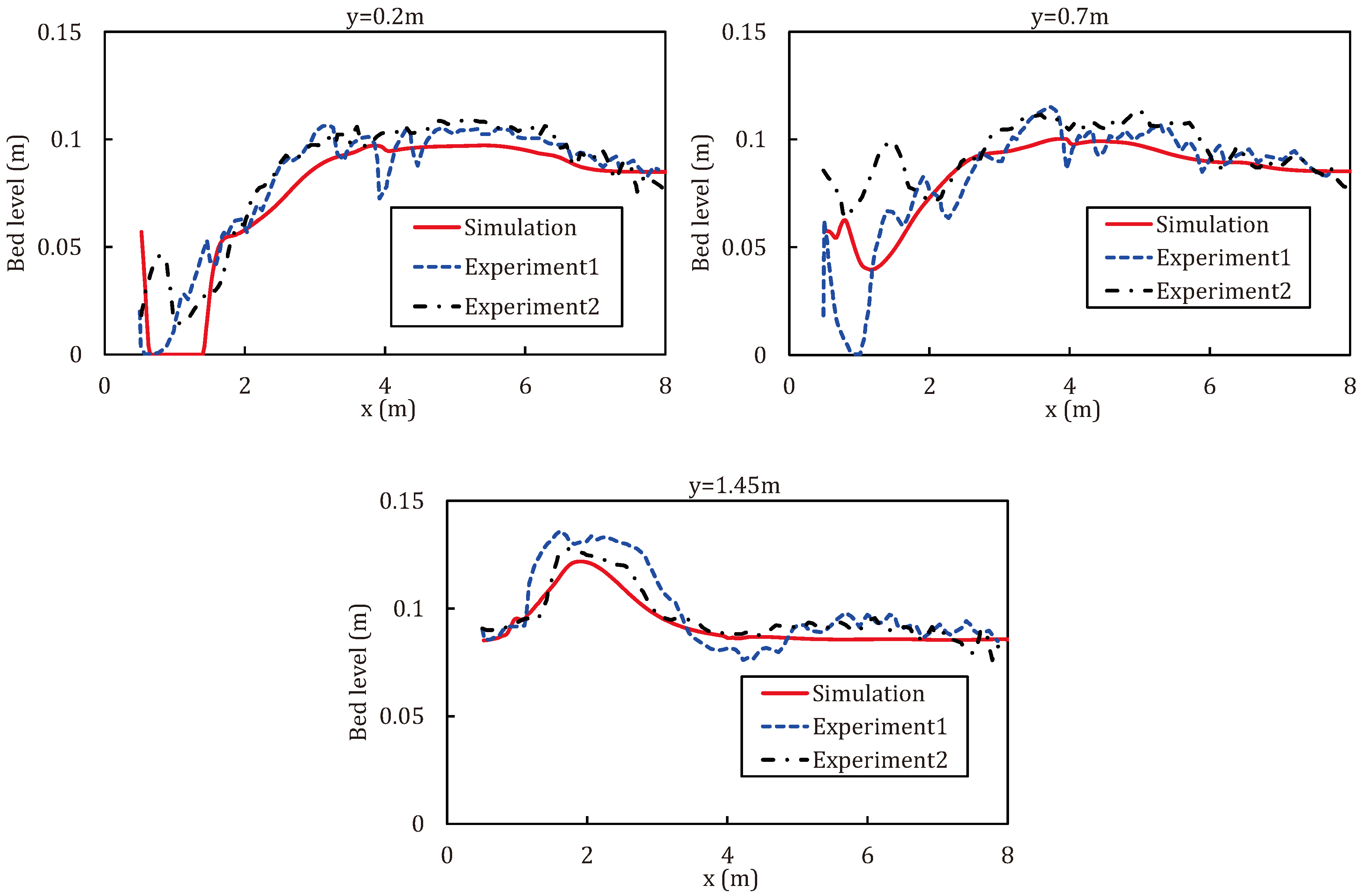
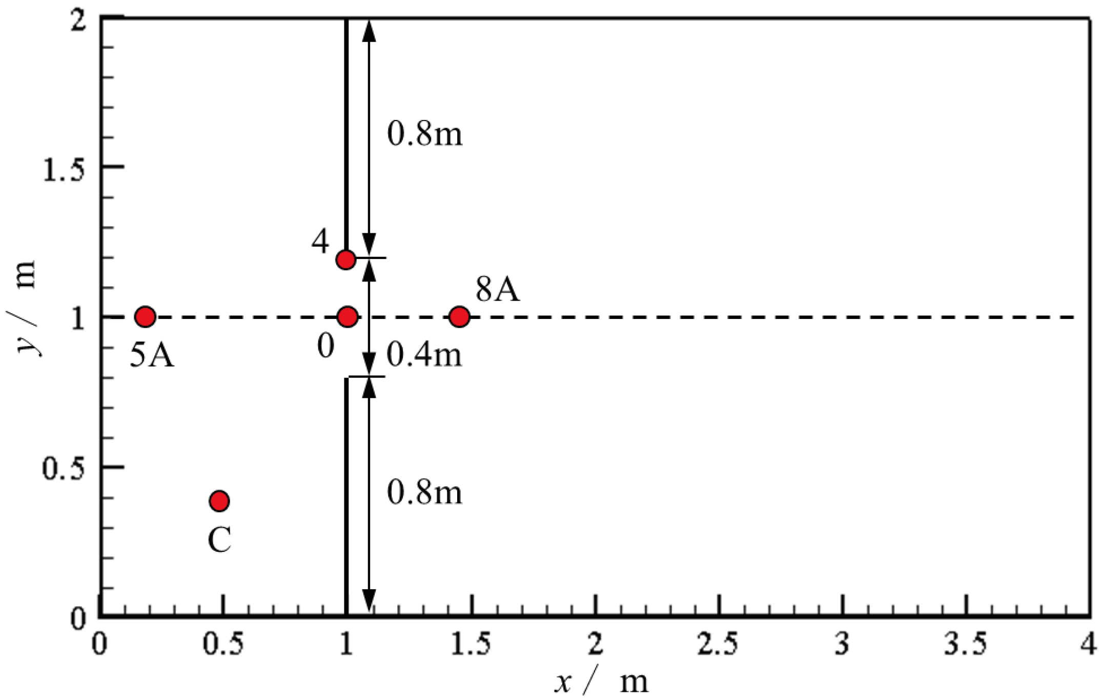
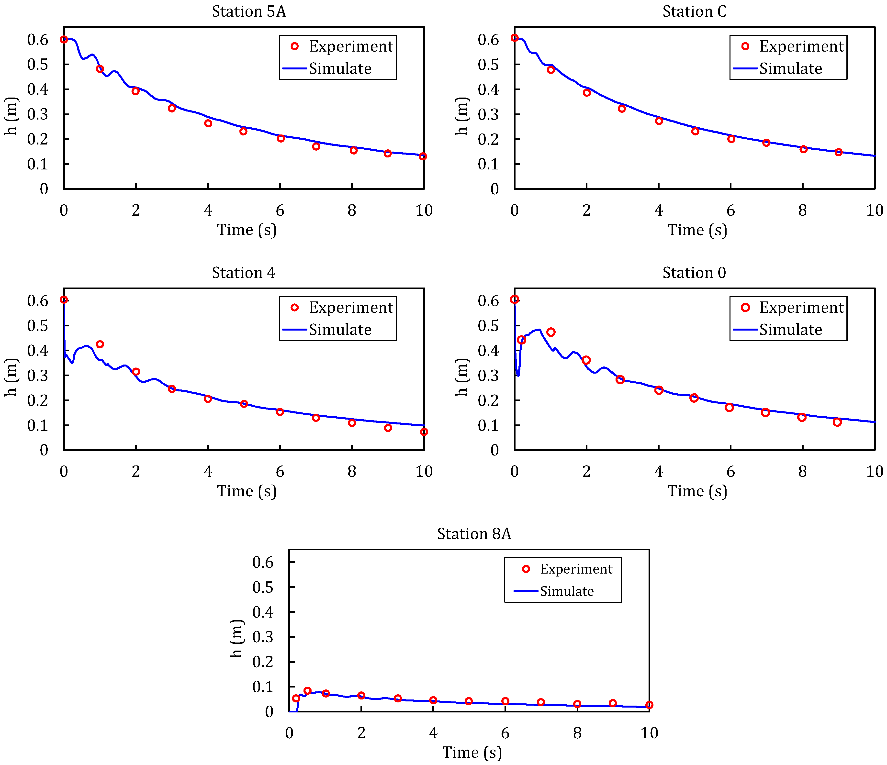
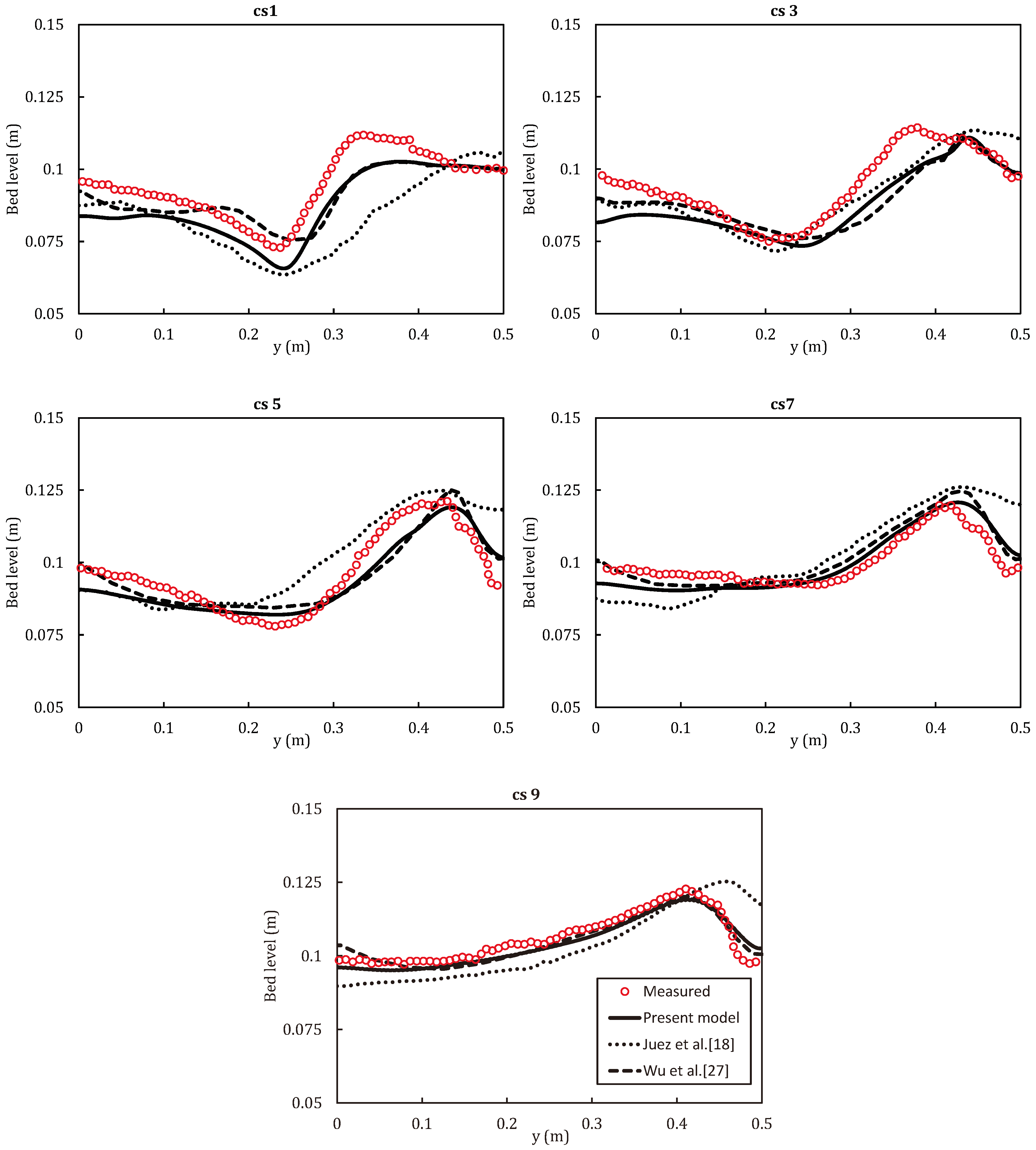
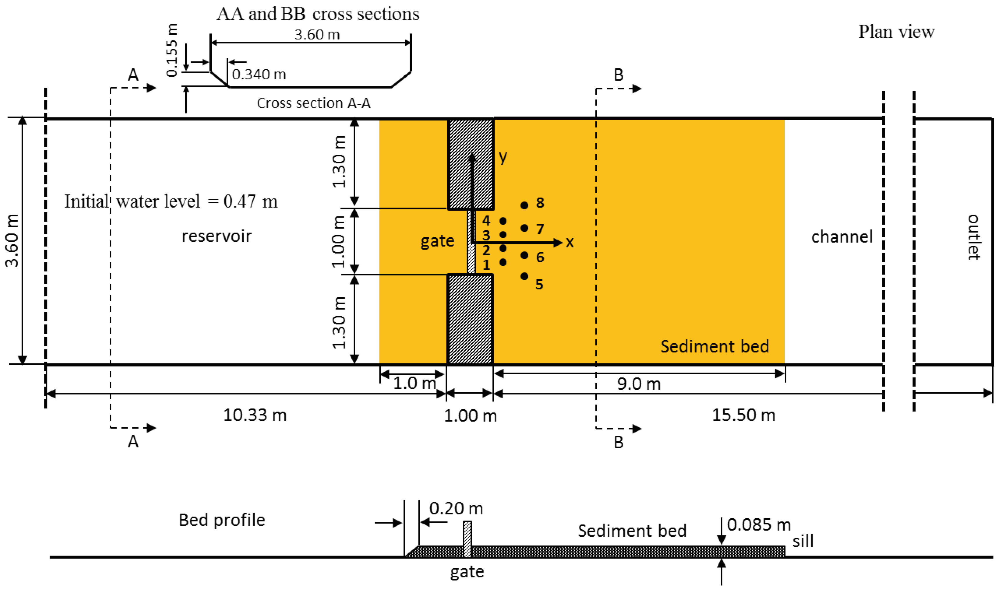
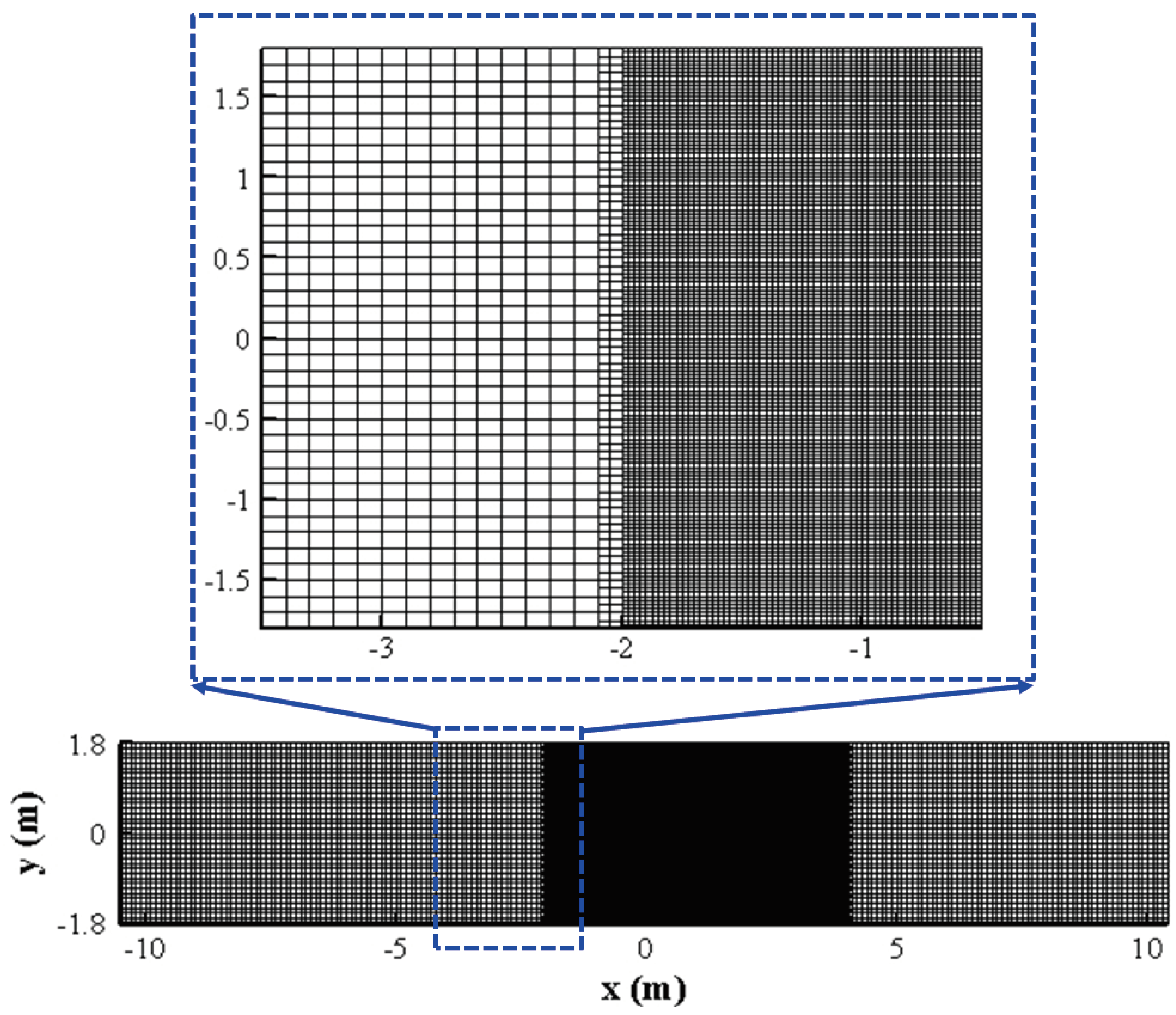
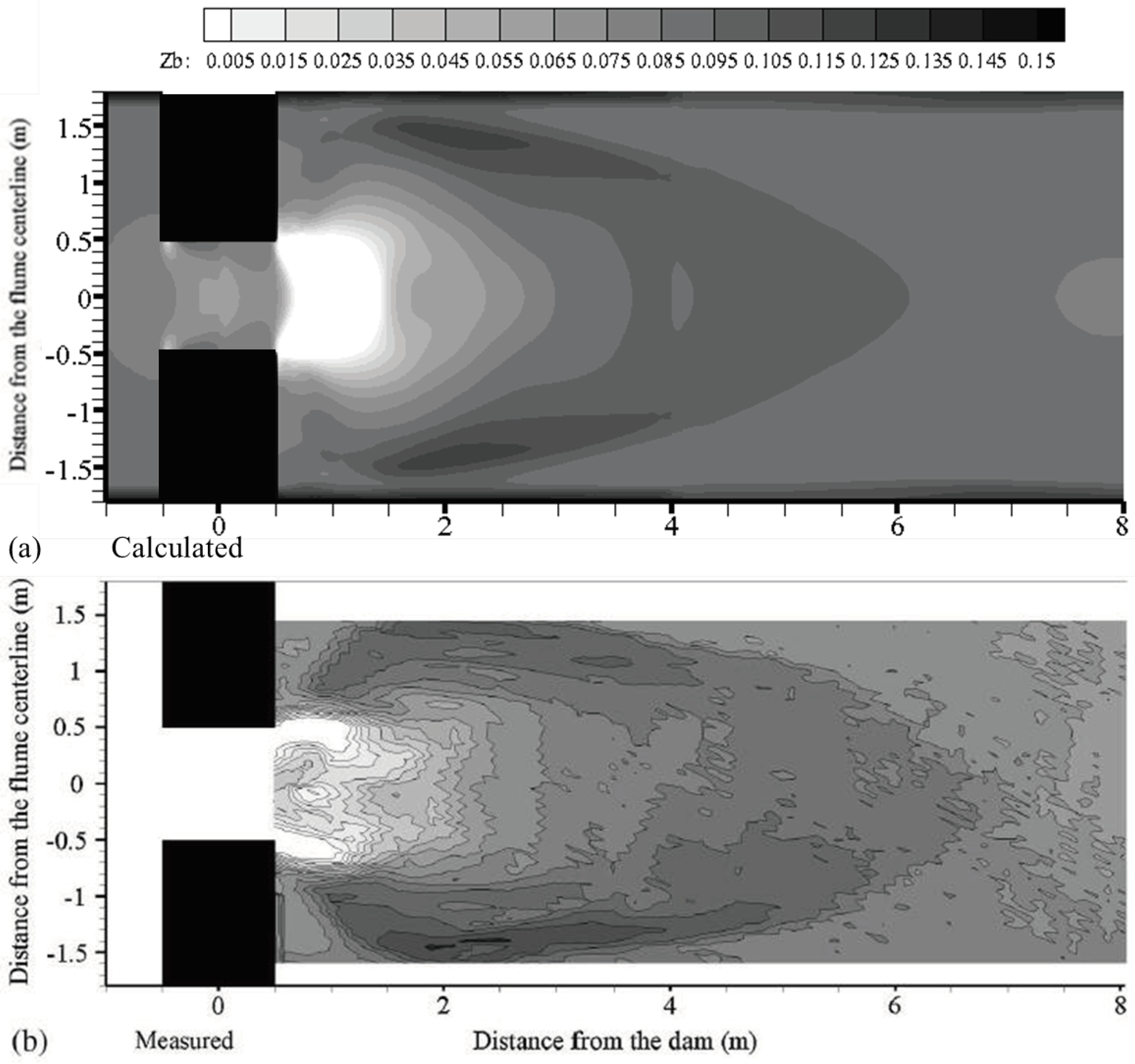
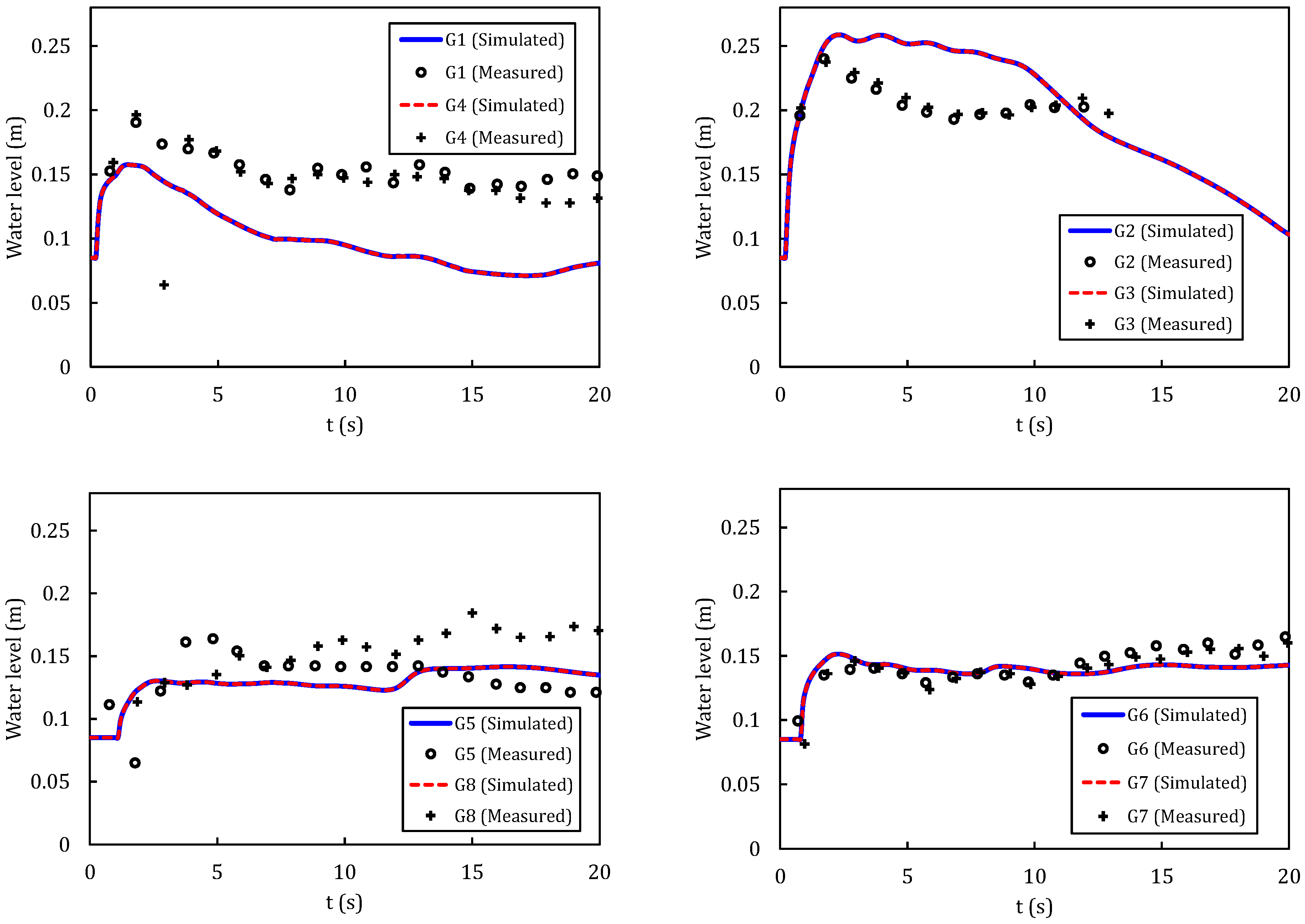
4.4. Partial Dam-Break Flow over Mobile Bed

In this section, the benchmark experiment of partial dam-break flow over mobile bed, which was also performed at UCL-Belgium [16] and has been used to test morphological models by many researchers [17,21,27,35,50], is adopted here to further verify the ability of the model to simulate bed evolution of a mobile bed caused by partial dam-break flow. As shown in Figure 13, the flume is 3.6 m wide and about 36 m long. The 1 m wide gate located between two impervious blocks is lifted immediately to represent partial dam-break. The gate center is set to be the origin of the Cartesian coordinate system. The fixed bed of the flume is paved with an 85 mm thick sand layer extending from 1 m upstream of the gate to 9 m downstream of the gate. The medium diameter, specific gravity and the initial porosity of the fully saturated sand lay are 1.61 mm, 2.63 and 0.42, respectively. The whole duration of the experiment is 20 s, which ensures the dam-break wave cannot reach the outlet and avoids the reflection effect from the downstream end of the flume. The initial water level in the upstream reservoir is 0.47 m and the downstream area is dry bed. Four pairs of ultrasonic gauges G1–G8 are symmetrically placed at downstream of the gate to measure the water level, and the coordinates of gauges are given in

Table 3. Coordinates of gauges for experiment of partial dam-break flow over mobile bed.

Gauges	G1	G2	G3	G4	G5	G6	G7	G8
x/m	0.64	0.64	0.64	0.64	1.94	1.94	1.94	1.94
y/m	−0.50	−0.165	0.165	0.50	−0.99	−0.33	0.33	0.99

. Bed profiles along three longitudinal sections (y = 0.2 m, 0.7 m, and 1.45 m) are measured at the end of the experiment.

As shown in Figure 14, a coarse mesh consisting of 360 × 36 rectangular grids ($\Delta x=\Delta y$ = 0.1 m) in longitudinal and lateral directions is firstly used to cover the whole domain. Then, the domain between 1.0 m upstream of the dam and 4.0 m downstream of the gate is refined and the subdivision level is 2. The Manning’s coefficient for the fixed bed and movable bed are equal to 0.01 and 0.0165, respectively [16]. Following the suggestion of Wu et al. [27], the calibrated value of the suspended-load adaptation coefficient $\alpha$ and the adaptation length of bed-load $L_b$ are set to be 4.0 and 0.025, respectively.

Figure 15 presents the calculated and measured bed elevation at the end of the experiment. Both of the measured and calculated results show that significant erosion occurs around the downstream of the gate which lead to a large scour hole, and some of the eroded sediment deposited along the sidewalls downstream of the hole. Although the erosion depth near the downstream of the dam is overestimated by the present model due to strong 3D features of the flow in this area, the computed and measured main erosion and deposition patterns are rather similar. Further quantitative comparisons between calculated and measured bed profile along three longitudinal sections (y = 0.2 m, 0.7 m and 1.45 m) are presented in Figure 16. Two sets of experimental bed elevation data (Experiment1 and Experiment2) measured using the same experimental setup are included in the figure. Strong variations between two experiments are observed, especially in the area between x = 0 m and x = 2 m. The possible reason for the difference between two repeated experiments is the random process of the turbulent flow. The average discrepancies $L_1$ of bed elevation along three longitudinal sections compared to the Experiment1 are 0.010 m, 0.012 m and 0.016 m, respectively. Compared to the Experiment2, the average discrepancies $L_1$ of bed elevation are 0.015 m, 0.011 m and 0.006 m, respectively. It should be noted that the deviations between calculated and measured bed elevation were in a similar magnitude with the discrepancy of the measured bed elevation among different experiment runs. In this respect, the computed bed elevations were generally in reasonable agreement with the measurements.

Figure 17 shows the calculated and measured water level at four pairs of gauges in a period of 20 s. It can be found that the calculated water levels at G1 and G4 are about 40 mm lower than the measurement, which are also reported by other researchers [27,35]. One possible reason is that strong 3D characteristics of the flow at the corners of the sudden expansion of the flume width cannot be resolved by 2D depth average hydrodynamic model. For the rest gauges, the calculated variations of water level agree with the measurement quite well. The average discrepancies $L_1$ of water level at four pairs of gauges (i.e., G1, G4, G2, G3, G5, G8, G6 and G7) are 0.054 m, 0.052 m, 0.031 m, 0.029 m, 0.018 m, 0.024 m, 0.010 m and 0.009 m, respectively.

5. Conclusions

In this paper, a depth-averaged 2D finite volume model based on non-uniform rectangular mesh has been developed to simulate dam break flow over movable beds. The model uses the enhanced shallow water equations which consider the effects of the mass and momentum exchange between flow phase and sediment phase. The non-equilibrium transport of total load is adopted in the sediment transport model. In the model, the non-uniform rectangular mesh is used to refine the grid in computational domains with complex flow structures, such as dam break locations. The fluxes at interface are calculated by the central-upwind scheme, which belongs to the class of Godunov-type Riemann-problem-solver-free central schemes and is able to capture the moving wet/dry fronts accurately. The nonnegative water depth reconstruction method is used to achieve second-order accuracy in space and C-property.

The developed model is firstly tested using two experimental cases of dam break flow over fixed irregular bed. The water depth and advance front celerity are well predicted by the present model. Then the model is further validated against two laboratory experiments of dam-break flow over movable bed. The comparison with the measurement data shows that the proposed model is able to calculate the water surface and final bed level generally well. In this study, the model is applied in the flume-scale dam-break flood with flow-sediment interaction. Since in reach-scale applications, the flow conditions and bed configurations are more complex, a further study of present model in real-life applications will be addressed.

References

1. Wu, W. Computational River Dynamics; Taylor & Francis: London, UK, 2008; Volume 78. [Google Scholar]
2. Fraccarollo, L.; Toro, E.F. Experimental and numerical assessment of the shallow water model for two-dimensional dam-break type problems. J. Hydraul. Res. 1995, 33, 843–864. [Google Scholar] [CrossRef]
3. Zhou, J.G.; Causon, D.M.; Mingham, C.G.; Ingram, D.M. The surface gradient method for the treatment of source terms in the shallow-water equations. J. Comput. Phys. 2001, 168, 1–25. [Google Scholar] [CrossRef]
4. Liang, Q. Flood simulation using a well-balanced shallow flow model. J. Hydraul. Eng. 2010, 136, 669–675. [Google Scholar] [CrossRef]
5. Song, L.; Zhou, J.; Li, Q.; Yang, X.; Zhang, Y. An unstructured finite volume model for dam-break floods with wet/dry fronts over complex topography. Int. J. Numer. Methods Fluids 2011, 67, 960–980. [Google Scholar] [CrossRef]
6. Wu, G.; He, Z.; Liu, G. Development of a cell-centered Godunov-type finite volume model for shallow water flow based on unstructured mesh. Math. Probl. Eng. 2014, 2014, 257915. [Google Scholar] [CrossRef]
7. Fraccarollo, L.; Capart, H. Riemann wave description of erosional dam-break flows. J. Fluid Mech. 2002, 461, 183–228. [Google Scholar] [CrossRef]
8. Spinewine, B.; Zech, Y. Small-scale laboratory dam-break waves on movable beds. J. Hydraul. Res. 2007, 45, 73–86. [Google Scholar] [CrossRef]
9. Cao, Z.; Pender, G.; Wallis, S.; Carling, P. Computational dam-break hydraulics over erodible sediment bed. J. Hydraul. Eng. 2004, 130, 689–703. [Google Scholar] [CrossRef]
10. Wu, W.; Wang, S.S. One-dimensional modeling of dam-break flow over movable beds. J. Hydraul. Eng. 2007, 133, 48–58. [Google Scholar] [CrossRef]
11. Abderrezzak, K.E.K.; Paquier, A.; Gay, B. One-dimensional numerical modelling of dam-break waves over movable beds: Application to experimental and field cases. Environ. Fluid Mech. 2008, 8, 169–198. [Google Scholar] [CrossRef]
12. Xia, J.; Lin, B.; Falconer, R.A.; Wang, G. Modelling dam-break flows over mobile beds using a 2D coupled approach. Adv. Water Resour. 2010, 33, 171–183. [Google Scholar] [CrossRef]
13. Benkhaldoun, F.; Sari, S.; Seaid, M. A flux-limiter method for dam-break flows over erodible sediment beds. Appl. Math. Model. 2012, 36, 4847–4861. [Google Scholar] [CrossRef]
14. Li, S.; Duffy, C.J. Fully coupled approach to modeling shallow water flow, sediment transport, and bed evolution in rivers. Water Resour. Res. 2011, 47. [Google Scholar] [CrossRef]
15. Liu, X.; Sedano, J.A.I.; Mohammadian, A. A robust coupled 2-D model for rapidly varying flows over erodible bed using central-upwind method with wetting and drying. Can. J. Civ. Eng. 2015, 42, 530–543. [Google Scholar] [CrossRef]
16. Soares-Frazão, S.; Canelas, R.; Cao, Z.; Cea, L.; Chaudhry, H.M.; Die Moran, A.; El Kadi, K.; Ferreira, R.; Cadórniga, I.F.; Gonzalez-Ramirez, N.; et al. Dam-break flows over mobile beds: Experiments and benchmark tests for numerical models. J. Hydraul. Res. 2012, 50, 364–375. [Google Scholar] [CrossRef]
17. Juez, C.; Murillo, J.; García-Navarro, P. Numerical assessment of bed-load discharge formulations for transient flow in 1D and 2D situations. J. Hydroinform. 2013, 15, 1234–1257. [Google Scholar] [CrossRef]
18. Juez, C.; Murillo, J.; García-Navarro, P. A 2D weakly-coupled and efficient numerical model for transient shallow flow and movable bed. Adv. Water Resour. 2014, 71, 93–109. [Google Scholar] [CrossRef]
19. Juez, C.; Ferrer-Boix, C.; Murillo, J.; Hassan, M.; García-Navarro, P. A model based on Hirano-Exner equations for two-dimensional transient flows over heterogeneous erodible beds. Adv. Water Resour. 2016, 87, 1–18. [Google Scholar] [CrossRef]
20. Juez, C.; Soares-Frazao, S.; Murillo, J.; García-Navarro, P. Experimental and numerical simulation of bed load transport over steep slopes. J. Hydraul. Res. 2017, 55, 455–469. [Google Scholar] [CrossRef]
21. He, Z.; Wu, T.; Weng, H.; Hu, P.; Wu, G. Numerical simulation of dam-break flow and bed change considering the vegetation effects. Int. J. Sediment Res. 2017, 32, 105–120. [Google Scholar] [CrossRef]
22. Di Cristo, C.; Evangelista, S.; Greco, M.; Iervolino, M.; Leopardi, A.; Vacca, A. Dam-break waves over an erodible embankment: Experiments and simulations. J. Hydraul. Res. 2018, 56, 196–210. [Google Scholar] [CrossRef]
23. Sánchez, A.; Wu, W. A non-equilibrium sediment transport model for coastal inlets and navigation channels. J. Coast. Res. 2011, 59, 39–48. [Google Scholar] [CrossRef]
24. Cao, Z.; Day, R.; Egashira, S. Coupled and decoupled numerical modeling of flow and morphological evolution in alluvial rivers. J. Hydraul. Eng. 2002, 128, 306–321. [Google Scholar] [CrossRef]
25. Greenberg, J.M.; LeRoux, A.Y. A well-balanced scheme for the numerical processing of source terms in hyperbolic equations. SIAM J. Numer. Anal. 1996, 33, 1–16. [Google Scholar] [CrossRef]
26. Bermudez, A.; Vázquez, M.E. Upwind methods for hyperbolic conservation laws with source terms. Comput. Fluids 1994, 23, 1049–1071. [Google Scholar] [CrossRef]
27. Wu, W.; Marsooli, R.; He, Z. Depth-averaged two-dimensional model of unsteady flow and sediment transport due to noncohesive embankment break/breaching. J. Hydraul. Eng. 2011, 138, 503–516. [Google Scholar] [CrossRef]
28. Kurganov, A.; Noelle, S.; Petrova, G. Semidiscrete central-upwind schemes for hyperbolic conservation laws and Hamilton–Jacobi equations. SIAM J. Sci. Comput. 2001, 23, 707–740. [Google Scholar] [CrossRef]
29. He, Z.; Hu, P.; Zhao, L.; Wu, G.; Pähtz, T. Modeling of breaching due to overtopping flow and waves based on coupled flow and sediment transport. Water 2015, 7, 4283–4304. [Google Scholar] [CrossRef]
30. Singh, J.; Altinakar, M.S.; Ding, Y. Two-dimensional numerical modeling of dam-break flows over natural terrain using a central explicit scheme. Adv. Water Resour. 2011, 34, 1366–1375. [Google Scholar] [CrossRef]
31. Kurganov, A.; Petrova, G. A second-order well-balanced positivity preserving central-upwind scheme for the Saint-Venant system. Commun. Math. Sci. 2007, 5, 133–160. [Google Scholar] [CrossRef]
32. Evangelista, S.; Altinakar, M.S.; Di Cristo, C.; Leopardi, A. Simulation of dam-break waves on movable beds using a multi-stage centered scheme. Int. J. Sediment Res. 2013, 28, 269–284. [Google Scholar] [CrossRef]
33. Liang, Q. A structured but non-uniform Cartesian grid-based model for the shallow water equations. Int. J. Numer. Methods Fluids 2011, 66, 537–554. [Google Scholar] [CrossRef]
34. Benkhaldoun, F.; Sahmim, S.; Seaid, M. A two-dimensional finite volume morphodynamic model on unstructured triangular grids. Int. J. Numer. Methods Fluids 2010, 63, 1296–1327. [Google Scholar] [CrossRef]
35. Huang, W.; Cao, Z.; Pender, G.; Liu, Q.; Carling, P. Coupled flood and sediment transport modelling with adaptive mesh refinement. Sci. China Technol. Sci. 2015, 58, 1425–1438. [Google Scholar] [CrossRef]
36. Zhang, M.; Wu, W. A two dimensional hydrodynamic and sediment transport model for dam break based on finite volume method with quadtree grid. Appl. Ocean Res. 2011, 33, 297–308. [Google Scholar] [CrossRef]
37. Wu, W.; Sánchez, A.; Zhang, M. An implicit 2-D shallow water flow model on unstructured quadtree rectangular mesh. J. Coas. Res. 2011, 15–26. [Google Scholar] [CrossRef]
38. Armanini, A.; Di Silvio, G. A one-dimensional model for the transport of a sediment mixture in non-equilibrium conditions. J. Hydraul. Res. 1988, 26, 275–292. [Google Scholar] [CrossRef]
39. Greimann, B.; Lai, Y.; Huang, J. Two-dimensional total sediment load model equations. J. Hydraul. Eng. 2008, 134, 1142–1146. [Google Scholar] [CrossRef]
40. Wu, W. Depth-averaged two-dimensional numerical modeling of unsteady flow and nonuniform sediment transport in open channels. J. Hydraul. Eng. 2004, 130, 1013–1024. [Google Scholar] [CrossRef]
41. Zhang, R.; Xie, J. Sedimentation Research in China: Systematic Selections; China Water and Power Press: Beijing, China, 1993. [Google Scholar]
42. Wu, W.; Wang, S.S.; Jia, Y. Nonuniform sediment transport in alluvial rivers. J. Hydraul. Res. 2000, 38, 427–434. [Google Scholar] [CrossRef]
43. Audusse, E.; Bouchut, F.; Bristeau, M.O.; Klein, R.; Perthame, B.T. A fast and stable well-balanced scheme with hydrostatic reconstruction for shallow water flows. SIAM J. Sci. Comput. 2004, 25, 2050–2065. [Google Scholar] [CrossRef]
44. Morris, M. CADAM: Concerted Action on Dam-Break Modeling—Final Report; Report SR 571; HR Wallingford: Wallingford, UK, 2000. [Google Scholar]
45. Liang, Q.; Marche, F. Numerical resolution of well-balanced shallow water equations with complex source terms. Adv. Water Resour. 2009, 32, 873–884. [Google Scholar] [CrossRef]
46. Brufau, P.; Garcia-Navarro, P. Two-dimensional dam break flow simulation. Int. J. Numer. Methods Fluids 2000, 33, 35–57. [Google Scholar] [CrossRef]
47. Liang, D.; Falconer, R.A.; Lin, B. Comparison between TVD-MacCormack and ADI-type solvers of the shallow water equations. Adv. Water Resour. 2006, 29, 1833–1845. [Google Scholar] [CrossRef]
48. Goutiere, L.; Soares-Frazão, S.; Zech, Y. Dam-break flow on mobile bed in abruptly widening channel: Experimental data. J. Hydraul. Res. 2011, 49, 367–371. [Google Scholar] [CrossRef]
49. Palumbo, A.; Soares-Frazao, S.; Goutiere, L.; Pianese, D.; Zech, Y. Dam-break flow on mobile bed in a channel with a sudden enlargement. River Flow 2008, 1, 645–654. [Google Scholar]
50. Canelas, R.; Murillo, J.; Ferreira, R.M. Two-dimensional depth-averaged modelling of dam-break flows over mobile beds. J. Hydraul. Res. 2013, 51, 392–407. [Google Scholar] [CrossRef]
Figure 1. Example of non-uniform rectangular mesh.
Water 10 00616 g001
Figure 2. Non-uniform rectangular control element i.
Water 10 00616 g002
Figure 3. The detailed setup of partial dam break experiment and positions of the gauges [2].
Water 10 00616 g003
Figure 4. The computational grids for partial dam break experiment.
Water 10 00616 g004
Figure 5. Comparisons between calculated and measured water depth at five gauge stations.
Water 10 00616 g005
Figure 6. The experimental setup of dam break flow over triangular obstacle [44].
Water 10 00616 g006
Figure 7. The computational grid for the dam break flow over triangular obstacle.
Water 10 00616 g007
Figure 8. Calculated and measured water depth at six gauges.
Water 10 00616 g008
Figure 9. The experimental configuration of dam break flow over movable bed in a sudden-expanded channel (dash lines: measurement cross sections; circles: ultrasonic gauges) [48,49].
Water 10 00616 g009
Figure 10. The computational grid for the dam break flow over an erodible channel with a sudden enlargement.
Water 10 00616 g010
Figure 11. The measured and calculated water level at gauge P1, P2, P3, P6 and P7 in a period of 12 s.
Water 10 00616 g011
Figure 12. The measured and calculated bed elevation at cross section cs1, cs3, cs5, cs7 and cs9.
Water 10 00616 g012
Figure 13. The experimental configuration of partial dam break flow over movable bed [16].
Water 10 00616 g013
Figure 14. The computational grid for the partial dam-break flow over mobile bed.
Water 10 00616 g014
Figure 15. Calculated (a) and measured (b) topography at t = 20 s.
Water 10 00616 g015
Figure 16. The measured and calculated bed profiles along three longitudinal sections.
Water 10 00616 g016
Figure 17. The measured and calculated water level at four pairs of ultrasonic gauges G1–G8.
Water 10 00616 g017