1. Introduction
Hydrological changes are mainly being associated with climate change and changes in land use and cover [
1,
2,
3]. Climate change has impacts on precipitation and evapotranspiration, which interfere with the amount of water available in the soil [
2]. However, changes in soil use can interfere with the contribution of rainfall to runoff, affecting the main hydrological components: groundwater recharge, surface runoff, evaporation, and infiltration [
4]. This is similar to what has been observed in the Tana Basin in Ethiopia, where declining native vegetation and agricultural expansion has altered groundwater flow and runoff, significantly affecting streamflow [
5].
The Grande River Basin has been the subject of hydrological modelling [
6,
7,
8,
9] due to its importance in the production of electric energy in Brazil. It is located in a region with a high demand for water resources, not only for hydroelectric plants, but also for industrial use and agriculture [
10]. Due to climate change and changes in land use and cover the water resources in the region are becoming growingly vulnerable. This has concerned the managers of the energy generation sector, and has been the focus of plans focused on water sustainability [
11].
According to studies conducted in the Rio Grande Basin region, the replacement of the remaining forests with grasslands could increase the streamflow rate by up to 157 mm year
−1, resulting in an increased flood risk [
6]. An increase in the average air temperature may also impact the average annual discharge of the rivers, and the change may vary between +8 and +51% in relation to the years 1961–1990 [
9]. However, Viola et al. [
7] showed a possible reduction in the flow between the years 2011 and 2040. From 2040 onwards, the average annual flow may increase. Similar results were found by Ribeiro Junior et al. [
8]. Hydrological changes are related to intra-annual changes in precipitation. In late winter and early spring, the period of recession of flow caused by reduced precipitation can affect the dynamics of groundwater, directly impacting the flow of rivers. In summer, the increase in rain can impact the flood regime [
7].
Hydrological modelling using the Soil and Water Assessment Tool (SWAT) has been widely used in other countries, and has presented valuable results for streamflow simulation. In Brazil, the application of SWAT in some regions is still limited, as in the Grande River Basin [
12]. Thus, the objectives of this study are: (1) to model the streamflow in the area of direct influence of the Furnas HPP reservoir; (2) to verify the performance of the SWAT model in the flow simulation of the region; (3) to contribute to the behaviour understanding of tropical zones; and (4) to model from an unpublished database that is of high complexity.
2. Materials and Methodology
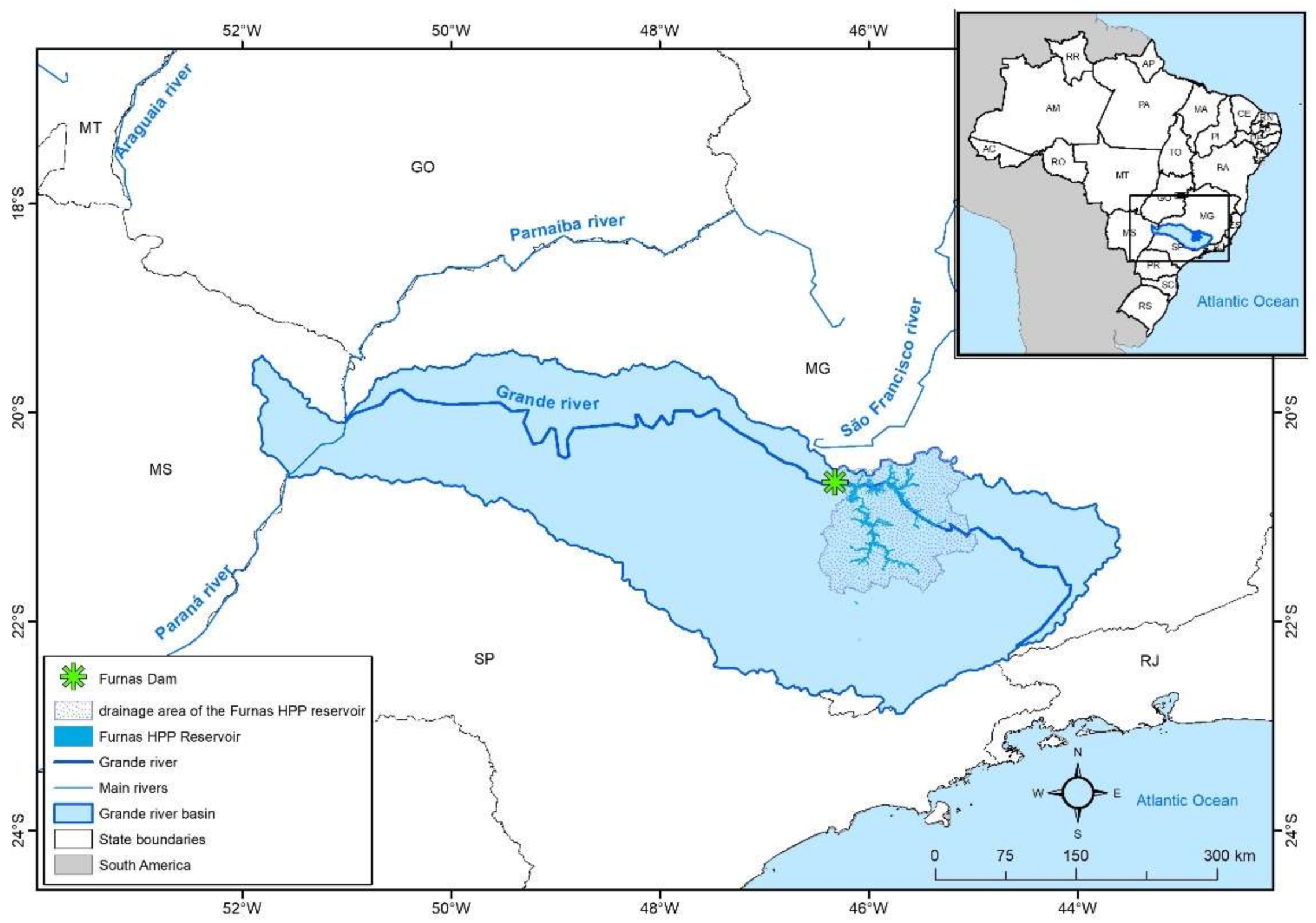
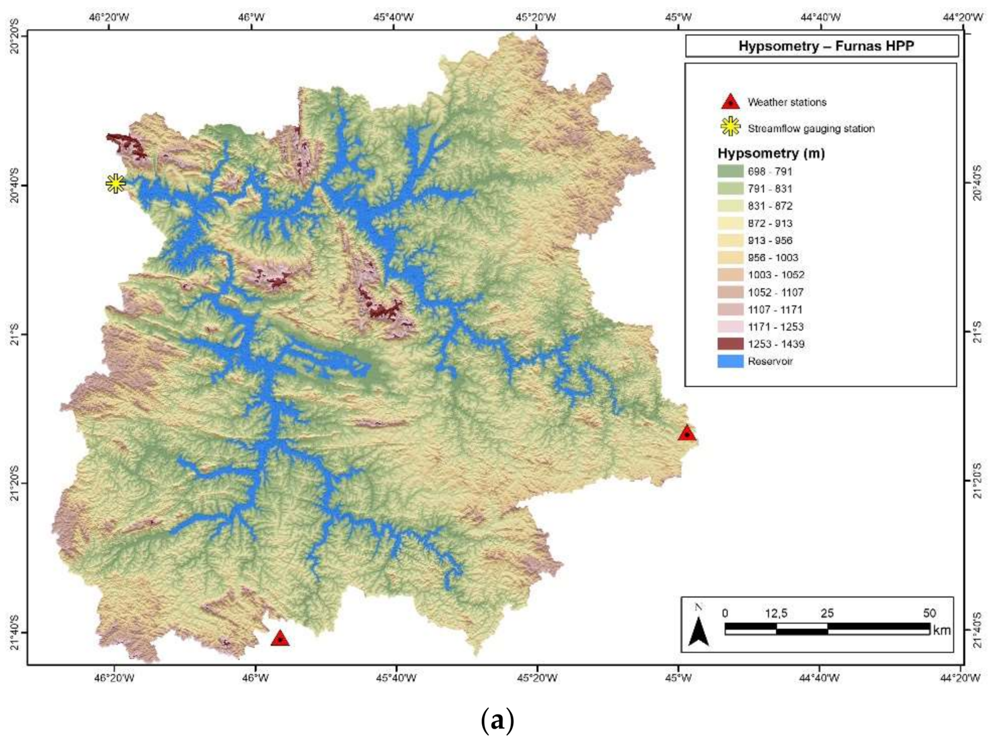
2.1. Area of Study
The study was carried out in the area of direct influence of the Furnas HPP reservoir (16,252 km
2). The reservoir is located in the Grande River Basin, in the southeastern region of Brazil (Latitude −20°67′ and Longitude −46°32′). The Furnas reservoir is one of the largest Brazilian reservoirs, with a maximum extension of 220 km and a usable volume of 17.217 billion m
3 of water, which has faced a significant reduction from 2012 [
13].
The predominant climate in the region is tropical of altitude (a variation of the tropical climate). It has the typical climate of mountainous regions, with rains in summer and drought in winter, as well as mild temperatures with narrow variations (annual averages between 21 and 23 °C) [
14] and an annual average precipitation between 16 and 296 mm. The location of the study area is shown in
Figure 1.
2.2. Hydrological Modelling
SWAT, version 2012, was used in the simulation of the Furnas reservoir’s streamflow. In the case of large basins, the SWAT model divides the basin into smaller areas (sub-basins). The limits of the basin, sub-basin, and flow network were defined based on the information provided by the Digital Elevation Model (DEM). An exclusion approach was adopted to control the number of HRUs (Hydrological Response Units); excluding areas of land use, soil types, and negligible slope degrees (minimum limits 20%, 10%, and 20%, respectively). Thus, 290 HRUs were generated combining the information on soil type, declivity, land use and land cover. In this study, the Curve Number (CN) method was adopted to estimate the surface runoff, while the Penman–Monteith method was used to estimate evapotranspiration.
2.3. Input Data for the Simulation
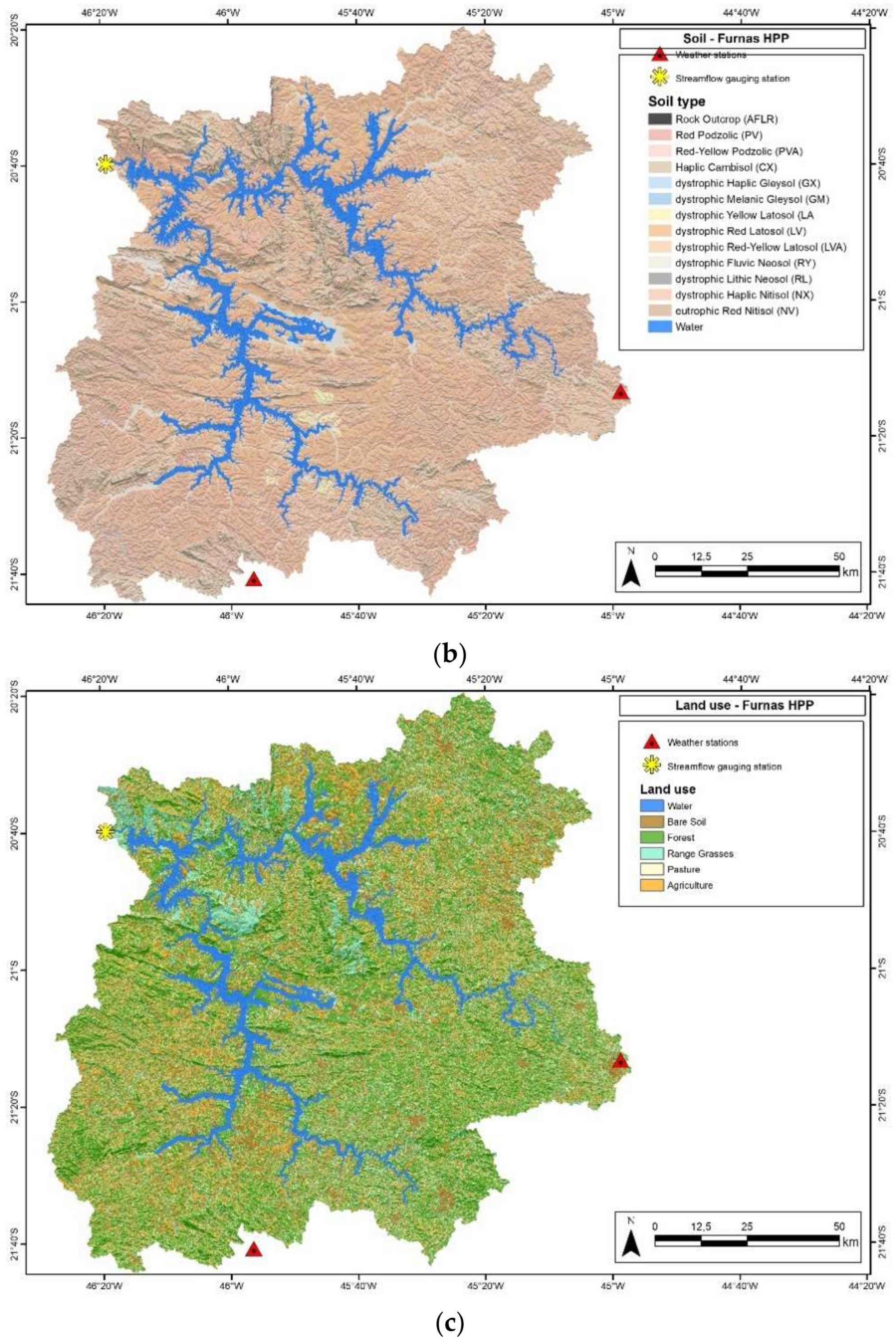
The data needed to develop the model were gathered by the following: The Digital Terrain Elevation Model (
Figure 2a); soil type (
Figure 2b); land use and land coverage data (
Figure 2c); and weather information. Georeferenced files were obtained through the State System of Geoinformations (SIEG). The files were treated using the ArcGIS software, associated with SWAT, and later thematic maps were generated.
Twelve categories of soil type were considered; where the most observed soils in the studied area were dystrophic Red Latosol (32.5%), dystrophic Red Argisol (19.8%), and dystrophic Haplic Cambisol (18.9%). The category of dystrophic Red Latosol presents the following main characteristics: high infiltration rate; high degree of resistance and tolerance to erosion; and low surface runoff potential. Physical–hydrological characteristics of the soil were obtained from the literature [
15,
16], due to the absence of field data for the study area. Based on the studies of Sartori et al. [
17], hydrologic soil groups were included. Each type of land use and cover was associated with the existing information in the SWAT database (
Table 1).
The climate data (precipitation, temperature, relative humidity, wind speed, and total insolation) of two weather stations (
Table 2) were extracted from the database of the Brazilian Institute of Meteorology [
18]. Total insolation data were used to calculate solar radiation [
19]. The historical series of climate data used incorporated a 16 year period (January 1998–December 2013). Existing faults were filled by the statistical climate generator function of SWAT (WXGEN). The necessary streamflow data for calibration and validation processes were obtained by the National Water Agency [
20] and the fluviometric station, located at the outlet of the Grande River Basin, in the drainage area of the Furnas reservoir. Mann–Kendall and Pettitt tests were applied to verify the behaviour of the data. The Mann–Kendall test verified the significance and direction of the data trend [
21], and the Pettitt test identified the change-point [
22]. The data decomposition was used to visualize the seasonal behaviour and changes in the trend over time.
2.4. Calibration and Validation of the Model
The processes of calibration and validation of the monthly streamflow were based on the general guidelines for the calibration protocol of the distributed models, as proposed by Abbaspour et al. [
23], and discussed by Rouholahnejad et al. [
24], Arnold et al. [
25], Abbaspour [
26], and Abbaspour et al. [
27]. The warm-up period of the model was two years (1998–1999), whereas, at least a year was required for the variables under study to be free of the initial conditions, as the uncertainties related to moisture [
25]. The calibration period was from 2000 to 2010 and the validation period 2011–2013.
Based on the relevant literature, the main parameters relating to hydrological processes to be included in the analysis of sensitivity, as well as the initial limits of these parameters [
25,
28], were identified. Some parameters, such as those relating to snow and temperature variation (SFTMP—Snowfall temperature, SMFMN—Minimum melt rate for snow during the year, SMFMX—Maximum melt rate for snow during, SMTMP—Snow melt base temperature, TIMP—Snow pack temperature lag factor, and TLAPS—Temperature laps rate), were not included, as they do not apply to the basin under study.
In the analysis of sensitivity and uncertainty, the SWAT-CUP software and the SUFI-2 algorithm were used. Through iterative processes, the algorithm performs the mapping of all uncertainties such as conceptual model, inputs the data and hydrologic parameters [
23]. The goodness-of-fit of the model was obtained by analysis of two indices: P-factor and R-factor. The P-factor is the percentage of the measured data bracketed by the 95% prediction of uncertainty (95PPU). The P-factor varies from 0 to 1. The R-factor indicates the thickness of the 95PPU and assesses the quality of calibration. The R-factor is the ratio of the average width of the 95PPU band and the standard deviation of the measured variable. In hydrological modelling, more specifically for streamflow, a P-factor greater than 0.7 and an R-factor less than 1.5 are desirable. The range of hydrological parameters was taken as calibrated when satisfactory values of the two factors were found, or when the objective function did not show improvement [
23,
24,
27].
In this study, the Nash-Sutcliffe coefficient was adopted as the objective function [
29,
30], as it’s one of the most widely used tests for calibration and validation of hydrological models [
12,
31,
32]. The application of the guidelines for evaluating the model performance varies according to the model calibration procedure, the quantity and quality of the measured data, and the evaluation time (monthly or daily) [
33]. Thus the Nash-Sutcliffe coefficient (Equation (1)) was adopted as the objective function as it fits the model for monthly streamflow, minimising the magnitude of the residual variance.
where
is streamflow observed;
is streamflow simulated;
is mean streamflow observed; and
n is the total number of observations.
NS values can vary between −∞ and 1.0, in which NS = 1 is considered a great value. Moriasi et al. [
33] presented the following classification for monthly assessments: NS > 0.75, model considered very good; 0.65 < NS ≤ 0.75, model considered good; 0.50 < NS ≤ 0.65, satisfactory model; NS ≤ 0.50, unsatisfactory model.
3. Results and Discussion
3.1. Statistical Analysis of Affluent Flow
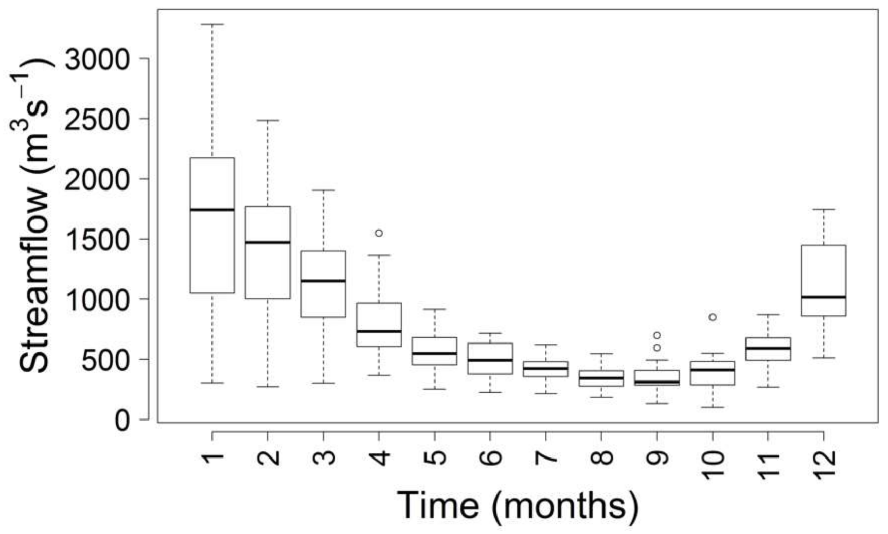
In the period from 2000 to 2015, the minimum recorded streamflow was 101 m3 s−1 (in 2014), and the maximum recorded streamflow was 3282 m3 s−1 (in 2007). The average recorded streamflow during this period was 772.20 m3·s−1, with a standard deviation of 561.27m3 s−1 and a variation coefficient of 72.69%; indicating a high variability in streamflow.
Streamflow variability was higher in January, February, March, and December (
Figure 3). The least amount of variability occurred between April and November; corresponding to the months of the year with smaller streamflow. In these months, the flow of the river is maintained by water reserves of groundwater, especially from aquifers, as is the case in Guarani, where the study area is located. A few outliers were observed in April, September, and October.
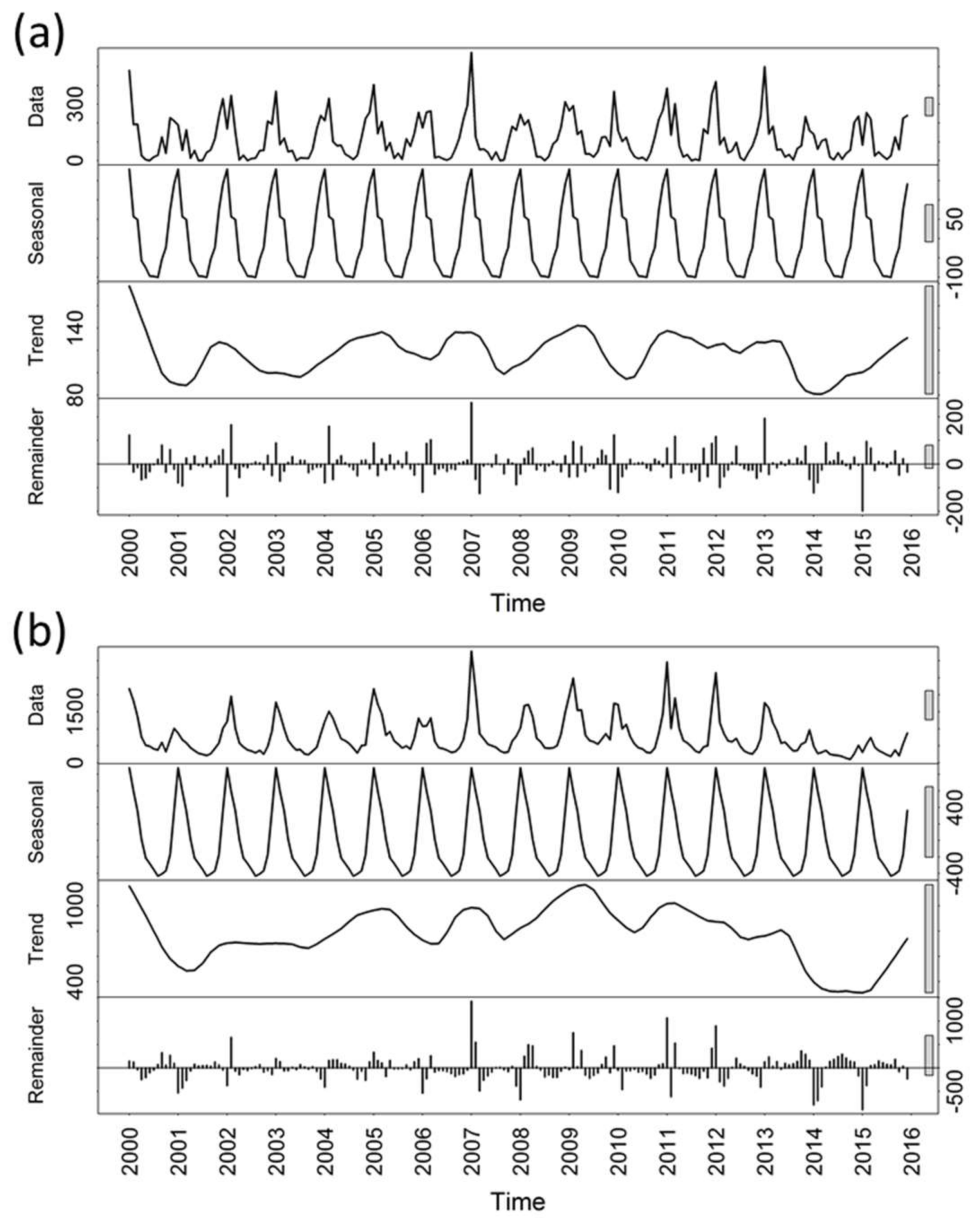
With a 95% certainty, the Mann–Kendall test shows that the streamflow tends to reduce (
p-value = 0.042). The decomposition in the series is presented to illustrate the seasonality of the region and its trend (
Figure 4). There is no tendency in precipitation (
p-value = 0.799). As this same trend is not presented with respect to precipitation, other factors may be affecting the reduction in streamflow in recent years, such as changes in land use and land cover, as well as the demand for irrigation upstream of the area under study [
5]. Thus, in the SWAT modelling, the years 2014 and 2015 were not used, because for model validation and calibration, the streamflow should have the same behavior [
34].
3.2. Calibration and Uncertainty Analysis
We considered the parameters of greater sensitivity in SWAT for the determination of streamflow [
25,
28], nine parameters presented greater sensitivity to the basin under study (
Table 3).
Arnold et al. [
25] pointed out that the parameters more frequently used in the calibration of surface runoff and base flow were CN2, SOL_AWC, ESCO, EPCO, SURLAG, OV_N, GW_ALPHA, GW_REVAP, GW_DELAY, GW_QMN, REVAPMIN, and RCHARG_DP.
The results of the sensitivity analysis (
Table 3) and the calibration (
Table 4) showed the importance of parameters, such as CN2 and ALPHA_BF (groundwater parameter) in the studied flow of the analysed region. The parameter CN2 is related to the quantity of runoff, and is based on the soil use, soil type, and the antecedents of humidity.
The analysis of the results (
Table 5), show that the positive values of PBIAS indicate a tendency of the model to underestimate the streamflow by 1.10%. Moreover, a NS value of 0.86, and a R2 value of 0.87, suggest that the model is suitable for the simulation of streamflow, based on the classification proposed by Moriasi et al. [
33].
The calibration of the model depends on factors such as the model inputs, the analyst’s assumptions, the model structure, and the calibration algorithm. Therefore, uncertainty analysis is required to assess the quality of fit that the model calibrated. In SWAT-CUP, the quality of the measurements is associated with the percentage of the observation points bracketed by the prediction uncertainty band (95PPU). Thus, high-quality measurements are considered to be those in which more than 80% of the measured data can be bracketed by the 95PPU. For instance, if only 50% of the data are bracketed for having uncertainty of prediction, it would indicate the existence of many outliers, and consequently the measurements would be considered of low quality [
23,
27].
For the streamflow calibration, 94% of the measured data were included in the bracketed of uncertainty of prediction (95PPU), with a 6% model error. The model satisfactorily estimated the streamflow in the Grande River Basin, but had some difficulties obtaining streamflow peaks and detecting small changes in the minimum streamflow.
It is worth mentioning that the parameters relating to land use were included from the available values of the SWAT database, which may have interfered with the adjustment of the model, specifically in relation to the minimum streamflow. In addition, the parameters of the soil types were adopted based on the relevant literature [
16].
In general, the model presents a good correlation between the precipitation and streamflow data, as shown in the hydrographs (
Figure 5). The greatest precipitation events were reflected in the peak streamflow, and the base streamflow was also well represented when the rainfall volume decreased.
The calibration assisted the improvement of the adjustment of minimum streamflow in relation to the initial simulation. The minimum observed streamflow (2000–2010) corresponded to 213 m
3 s
−1, which occurred in 2001, a period of energy crisis in Brazil. For this same period, the minimum simulated streamflow corresponded to 15 m
3 s
−1. Peak adjustment efficiency was not significant, the peaks were underestimated or overestimated over the years, corresponding to 3282 m
3 s
−1 for observed streamflow and 3267 m
3·s
−1 for simulated streamflow. The difficulties relating to the adjustment of the streamflow peaks are likely due to the high spatial and temporal variability of precipitation in the study area [
35].
3.3. Model Validation
In the model validation step the same hydrological parameters set during calibration were used, the climatic parameters were changed to function with the new period of data used: January 2011–December 2013. The hydrographs (
Figure 5) represent the simulated streamflow behaviour, in relation to the observed streamflow and the uncertainties of the model (95PPU).
Overall, the observed streamflow matched well with the simulated streamflow; although there were difficulties representing some of the streamflow peaks during the validation period; some variation was also observed during the calibration period. The model failed to satisfactorily represent in the validation stage; mainly in the streamflow peak observed in 2012.
The values of the statistical coefficients (NS and R2) for the validation period were considerably smaller than the values found for the calibration (
Table 5). However, the model was considered satisfactory according to the classification proposed by Moriasi et al. [
33].
The P-factor ranged from 0.94 (calibration) to 0.69 (validation), and the R-factor ranged from 1.59 (calibration) to 1.53 (validation). Abbaspour et al. [
23] recommended the adoption of a value of P-factor greater than 0.7, and a value of R-factor smaller than 1.5. Nevertheless, the authors highlighted that these values may vary depending on the suitability of the input data and model calibration.
Ghobadi et al. [
36] simulated the hydrological processes of the Karkheh river basin, Iran, using the SWAT-CUP for the calibration process and the analysis of uncertainties; the authors obtained values of the model assessment parameters that were slightly below the recommended values. They correlated the inaccuracies of the simulated results with the inadequate accounting of water use in the agricultural and industrial areas of the basin under analysis.
Pereira et al. [
35], used trial-and-error processes during the calibration and validation of hydrological modelling when applied to daily streamflow of the Pomba River Basin, Brazil, and obtained acceptable results according to the literature: a NS value of 0.76 and a PBIAS value of 4.6% during calibration; and a NS value of 0.76 and a PBIAS value of 5.1% during validation. These results indicate that the values of peak streamflow would be better represented if there were improvements in the representativeness of the precipitation.
According to Abbaspour et al. [
27], a watershed model cannot be fully validated, as there may be conditions in the watershed that are not taken in consideration during modelling (e.g., changes to the use of water for irrigation). Concurring with the authors, these uncertainties can lead to unsatisfactory results and make validation a major challenge to the model analyst.
Faramarzi et al. [
37], commented that the uncertainties in hydrological modelling may be related to factors such as irrigation; wastewater discharges (urban and industrial); interaction between surface water and groundwater. Abbaspour et al. [
24] added to these uncertainties: the quality of input data. Setegn et al. [
38] highlighted the critical aspects of the uncertainties in relation to climatic parameters; especially precipitation and temperature.
4. Discussions
In this study, the hydrological SWAT model was used to simulate the streamflow of the Furnas HPP reservoir. The performance of the SWAT model for the simulation of the affluent flow was statistically satisfactory; indicating that the model is able to represent the hydrological processes of the basin under study, and can be used in scenario analysis. Thus, its application can help to determine the policies for use and occupation of the soil surrounding the basin, and for the management of water resources in the region. This has the potential to directly impact the availability of water for power generation. Based on that information, managers can conduct hydrological assessments allowing adaptation strategies.
The model produced more satisfactory results for calibration than for validation, which may be related to the representativeness of the precipitation data and other conditions that are not modelled, such as the use of water for irrigation. For a better estimate of the extreme streamflow values, the model needs to be improved, specifically, the representativeness of the precipitation; the model needs to take into account data from rainfall stations over larger ranges, in order to be more thoroughly distributed throughout the basin.
The historical series analysis showed a trend of affluent flow reduction, which was reflected in the useful volume of the Furnas HPP reservoir for the same years. This trend of reduction was not clearly identified in the breakdown of the historical series of precipitation. Although rainfall is one of the main variables that influences streamflow (especially in extreme values), there are other factors that may interfere in the reduction of the streamflow rate of the studied basin, such as the increase in water volume used for agricultural irrigation, and the changes in land use and land coverage; justifying the tendency for the reduction in the affluent flow.
The determination of more sensitive hydrological parameters contributed to a better understanding of the hydrological regime in the watershed. Thus, the parameters that most interfered with the streamflow prediction results were identified (e.g., CN2, CH_N1, and ALPHA_BF). These parameters are related to the contribution of groundwater to runoff, and consequently to streamflow.
5. Conclusions
One of the limitations to the application of SWAT modelling in the Grande River Basin was the data availability, primarily of historical series of precipitation and streamflow. This limitation is related to the limited number of measurement stations, their distribution along the basin, and the size of the time series. More satisfactory data availability, would allow for better spatial representativeness of rainfall and better calibration of the different sub-basins, improving predictions and decreasing uncertainties.
The database used in the simulations is robust and unprecedented for Brazil, and the study has had a considerable contribution to the country. This is because hydroelectric plants are the main sources of electricity, and one of the main sources of renewable energy. However, few hydroelectric plants have this kind of data base to subsidize their maintenance and generation potential. In addition, this is an important collaboration for areas located in a tropical climate region, such as Brazil.
Acknowledgments
The work was supported by the National Council of Scientific and Technological Development (CNPq), through the program Science without Borders, and the National Agency of Electric Power (ANEEL)—Project and Development code 0394-1014-2010, through the Eletrobras Furnas Company, both from Brazil’s government. The authors gratefully acknowledge IESA-UFG (Institute of Socio-environmental Studies of the Federal University of Goiás) for soil data, classifications and map making.
Author Contributions
Viviane de Souza Dias, Marta Pereira da Luz, and Gabriela Maluf Medero performed the experiments and wrote the paper. Diego Tarley Ferreira Nascimento developed the GIS maps. Wellington Nunes de Oliveira and Leonardo Rodrigues de Oliveira Merelles assisted in the paper preparation.
Conflicts of Interest
The authors declare no conflict of interest.
References
- Li, F.; Zhang, G.; Xu, Y. Assessing climate change impacts on water resources in the Songhua river basin. Water 2016, 8, 420. [Google Scholar] [CrossRef]
- Worqlul, A.; Taddele, Y.; Ayana, E.; Jeong, J.; Adem, A.; Gerik, T. Impact of climate change on streamflow hydrology in headwater catchments of the Upper Blue Nile basin, Ethiopia. Water 2018, 10, 120. [Google Scholar] [CrossRef]
- Zhang, L.; Nan, Z.; Yu, W.; Ge, Y. Modeling land-use and land-cover change and hydrological responses under consistent climate change scenarios in the Heihe River Basin, China. Water Resour. Manag. 2015, 29, 4701–4717. [Google Scholar] [CrossRef]
- Sajikumar, N.; Remya, R.S. Impact of land cover and land use change on runoff characteristics. J. Environ. Manag. 2015, 161, 460–468. [Google Scholar] [CrossRef] [PubMed]
- Woldesenbet, T.A.; Elagib, N.A.; Ribbe, L.; Heinrich, J. Hydrological responses to land use/cover changes in the source region of the Upper Blue Nile Basin, Ethiopia. Sci. Total Environ. 2017, 575, 724–741. [Google Scholar] [CrossRef] [PubMed]
- Viola, M.R.; Mello, C.R.; Beskow, S.; Norton, L.D. Impacts of land-use changes on the hydrology of the Grande River basin headwaters, Southeastern Brazil. Water Resour. Manag. 2014, 28, 4537–4550. [Google Scholar] [CrossRef]
- Viola, M.R.; de Mello, C.R.; Chou, S.C.; Yanagi, S.N.; Gomes, J.L. Assessing climate change impacts on Upper Grande River Basin hydrology, Southeast Brazil. Int. J. Climatol. 2015, 35, 1054–1068. [Google Scholar] [CrossRef]
- Ribeiro Junior, L.U.; Zuffo, A.C.; Silva, B.C. Development of a tool for hydroeletric reservoir operation with multiple uses considering effects of climate changes. Case study of Furnas HPP. Rev. Bras. Recur. Hídr. 2016, 21, 300–313. [Google Scholar] [CrossRef]
- Nóbrega, M.T.; Collischonn, W.; Tucci, C.E.M.; Paz, A.R. Uncertainty in climate change impacts on water resources in the Rio Grande basin, Brazil. Hydrol. Earth Syst. Sci. 2011, 15, 585–595. [Google Scholar] [CrossRef]
- ANA (Agência Nacional de Águas). Região Hidrográfica do Paraná. Available online: http://www2.ana.gov.br/Paginas/portais/bacias/parana.aspx (accessed on 17 July 2016). (In Portuguese)
- ANA (Agência Nacional de Águas). Comitê Aprova Plano de Recursos Hídricos da Bacia do Rio Grande. Available online: http://www3.ana.gov.br/portal/ANA/noticias/comite-aprova-plano-integrado-de-recursos-hidricos-da-bacia-do-rio-grande (accessed on 20 March 2018). (In Portuguese)
- Bressiani, D.A.; Gassman, P.W.; Fernandes, J.G.; Garbossa, L.H.P.; Srinivasan, R.; Bonumá, N.B.; Mendiondo, E.M. A review of soil and water assessment tool (SWAT) applications in Brazil: Challenges and prospects. Int. J. Agric. Biol. Eng. 2015, 8, 9–35. [Google Scholar] [CrossRef]
- FURNAS Parque Gerador: Usina Hidrelétrica de Furnas. Available online: http://www.furnas.com.br/hotsites/sistemafurnas/usina_hidr_furnas.asp (accessed on 17 July 2016). (In Portuguese).
- CBH. Comitê Da Bacia Hidrográfica do Rio Grande Comitê Da Bacia Hidrográfica do Entorno do Lago de Furnas. Available online: http://www.grande.cbh.gov.br/GD3.aspx (accessed on 17 July 2016). (In Portuguese)
- Baldissera, G.C. Aplicabilidade do Modelo de Simulação Hidrológica SWAT (Soil and Water Assessment Tool), Para a Bacia Hidrográfica do Rio Cuiabá/MT. Master’s Thesis, Universidade Federal do Mato Grosso, Cuiabá, Brazil, 2005. (In Portuguese). [Google Scholar]
- Rosa, D.R.Q. Modelagem Hidrossedimentológica Na Bacia Hidrográfica do Rio Pomba Utilizando o SWAT. Ph.D. Thesis, Universidade Federal de Viçosa, Viçosa, Brazil, 2016. (In Portuguese). [Google Scholar]
- Sartori, A.; Neto, F.L.; Genovez, A.M. Classificação hidrológica de solos brasileiros para a estimativa da chuva excedente com o método do serviço de conservação do solo dos Estados Unidos Parte 1: Classificação. Rev. Bras. Recur. Hídr. 2005, 10, 5–18. (In Portuguese) [Google Scholar]
- INMET. Instituto Nacional de Meteorologia Banco de Dados Meteorológicos Para Ensino E Pesquisa (BDMEP). Available online: http://www.inmet.gov.br/portal/index.php?r=%0Abdmep/bdmep%0A (accessed on 17 July 2016). (In Portuguese)
- Allen, R.G.; Pereira, L.S.; Raes, D.; Smith, M.; Ab, W. Crop Evapotranspiration—Guidelines for Computing Crop Water Requirements—FAO Irrigation and Drainage Paper 56; FAO: Rome, Italy, 1998; pp. 1–15. [Google Scholar]
- ANA. Agência Nacional de Águas. Sistema de Acompanhamento de Reservatórios (SAR). Available online: http://sar.ana.gov.br/MedicaoSIN (accessed on 2 January 2017). (In Portuguese)
- Libiseller, C.; Grimvall, A. Performance of partial Mann-Kendall tests for trend detection in the presence of covariates. Environmetrics 2002, 13, 71–84. [Google Scholar] [CrossRef]
- Verstraeten, G.; Poesen, J.; Demarée, G.; Salles, C. Long-term (105 years) variability in rain erosivity as derived from 10-min rainfall depth data for Ukkel (Brussels, Belgium): Implications for assessing soil erosion rates. J. Geophys. Res. 2006, 111, 1–11. [Google Scholar] [CrossRef]
- Abbaspour, K.C.; Rouholahnejad, E.; Vaghefi, S.; Srinivasan, R.; Yang, H.; Kløve, B. A continental-scale hydrology and water quality model for Europe: Calibration and uncertainty of a high-resolution large-scale SWAT model. J. Hydrol. 2015, 524, 733–752. [Google Scholar] [CrossRef]
- Rouholahnejad, E.; Abbaspour, K.C.; Vejdani, M.; Srinivasan, R.; Schulin, R.; Lehmann, A. A parallelization framework for calibration of hydrological models. Environ. Model. Softw. 2012, 31, 28–36. [Google Scholar] [CrossRef]
- Arnold, J.G.; Moriasi, D.N.; Gassman, P.W.; Abbaspour, K.C.; White, M.J.; Srinivasan, R.; Santhi, C.; Harmel, R.D.; Van Griensven, A.; Van Liew, M.W.; et al. SWAT: Model use, calibration and validation. Am. Soc. Agric. Biol. Eng. 2012, 55, 1491–1508. [Google Scholar]
- Abbaspour, K.C. SWAT CUP—SWAT Calibration and Uncertainty Programs. Available online: http://swat.tamu.edu/media/114860/usermanual_swatcup.pdf (accessed on 3 January 2017).
- Abbaspour, K.C.; Yang, J.; Maximov, I.; Siber, R.; Bogner, K.; Mieleitner, J.; Zobrist, J.; Srinivasan, R. Modelling hydrology and water quality in the pre-alpine/alpine Thur watershed using SWAT. J. Hydrol. 2007, 333, 413–430. [Google Scholar] [CrossRef]
- Van Griensven, A.; Meixner, T.; Grunwald, S.; Bishop, T.; Diluzio, M.; Srinivasan, R. A global sensitivity analysis tool for the parameters of multi-variable catchment models. J. Hydrol. 2006, 324, 10–23. [Google Scholar] [CrossRef]
- Gupta, H.V.; Sorooshian, S.; Yapo, P.O. Status of automatic calibration for hydrologic model: Comparison with multilevel expert calibration. J. Hydrol. Eng. 1999, 4, 135–143. [Google Scholar] [CrossRef]
- Nash, J.E.; Sutchiffe, J.V. River flow forecasting through conceptual models part I—A discussion of principles. J. Hydrol. 1970, 10, 282–290. [Google Scholar] [CrossRef]
- Du, J.; Rui, H.; Zuo, T.; Li, Q.; Zheng, D.; Chen, A.; Xu, Y.; Xu, C.Y. Hydrological simulation by SWAT model with fixed and varied parameterization approaches under land use change. Water Resour. Manag. 2013, 27, 2823–2838. [Google Scholar] [CrossRef]
- Yen, H.; Jeong, J.; Feng, Q.; Deb, D. Assessment of input uncertainty in SWAT using latent variables. Water Resour. Manag. 2015, 29, 1137–1153. [Google Scholar] [CrossRef]
- Moriasi, D.N.; Arnold, J.G.; Van Liew, M.W.; Bingner, R.L.; Harmel, R.D.; Veith, T.L. Model evaluation guidelines for systematic quantification of accuracy in watershed simulation. Am. Soc. Agric. Biol. Eng. 2007, 50, 885–900. [Google Scholar]
- Abbaspour, K.; Vaghefi, S.; Srinivasan, R. A guideline for successful calibration and uncertainty analysis for soil and water assessment: A review of papers from the 2016 International SWAT Conference. Water 2018, 10, 6. [Google Scholar] [CrossRef]
- Pereira, D.R.; Martinez, M.A.; Pruski, F.F.; Demetrius, D.S. Hydrological simulation in a basin of typical tropical climate and soil using the SWAT model part I : Calibration and validation tests. J. Hydrol. Reg. Stud. 2016, 7, 14–37. [Google Scholar] [CrossRef]
- Ghobadi, Y.; Pradhan, B.; Abbas, G.; Kabiri, K.; Yashar, F. Simulation of hydrological processes and effects of engineering projects on the Karkheh River Basin and its wetland using SWAT2009. Quat. Int. 2015, 374, 144–153. [Google Scholar] [CrossRef]
- Faramarzi, M.; Abbaspour, K.C.; Schulin, R.; Yang, H. Modelling blue and green water resources availability in Iran. Hydrol. Process. 2009, 23, 486–501. [Google Scholar] [CrossRef]
- Setegn, S.G.; Srinivasan, R.; Dargahi, B. Hydrological modelling in the Lake Tana Basin, Ethiopia using SWAT model. Open Hydrol. J. 2008, 2, 49–62. [Google Scholar] [CrossRef]
© 2018 by the authors. Licensee MDPI, Basel, Switzerland. This article is an open access article distributed under the terms and conditions of the Creative Commons Attribution (CC BY) license (http://creativecommons.org/licenses/by/4.0/).

 ,
, 


