Tracers Reveal Recharge Elevations, Groundwater Flow Paths and Travel Times on Mount Shasta, California


1
Department of Earth and Environmental Sciences, California State University East Bay, Hayward, CA 94542, USA
2
Lawrence Livermore National Laboratory, Livermore, CA 94550, USA
*
Author to whom correspondence should be addressed.
Water 2018, 10(2), 97; https://doi.org/10.3390/w10020097
Submission received: 31 October 2017
/
Revised: 17 January 2018
/
Accepted: 18 January 2018
/
Published: 23 January 2018
(This article belongs to the Special Issue Isotopes in Hydrology and Hydrogeology)
Abstract
:Mount Shasta (4322 m) is famous for its spring water. Water for municipal, domestic and industrial use is obtained from local springs and wells, fed by annual snow melt and sustained perennially by the groundwater flow system. We examined geochemical and isotopic tracers in samples from wells and springs on Mount Shasta, at the headwaters of the Sacramento River, in order to better understand the hydrologic system. The topographic relief in the study area imparts robust signatures of recharge elevation to both stable isotopes of the water molecule (δ18O and δD) and to dissolved noble gases, offering tools to identify recharge areas and delineate groundwater flow paths. Recharge elevations determined using stable isotopes and noble gas recharge temperatures are in close agreement and indicate that most snowmelt infiltrates at elevations between 2000 m and 2900 m, which coincides with areas of thin soils and barren land cover. Large springs in Mt Shasta City discharge at an elevation more than 1600 m lower. High elevation springs (>2000 m) yield very young water (<2 years) while lower elevation wells (1000–1500 m) produce water with a residence time ranging from 6 years to over 60 years, based on observed tritium activities. Upslope movement of the tree line in the identified recharge elevation range due to a warming climate is likely to decrease infiltration and recharge, which will decrease spring discharge and production at wells, albeit with a time lag dependent upon the length of groundwater flow paths.
1. Introduction
A warming climate will bring drastic changes to hydrologic systems in the headwater basins of the major rivers in California. Runoff in these rivers fills the reservoirs that sustain cities and agriculture through the dry months, while cool, late season groundwater discharge to streams is critical for sustaining subalpine ecosystems and fish habitat. Despite the important role they play in the larger hydrologic system, interactions between surface water and groundwater in headwater basins and mountainous regions are typically not well characterized, with recharge locations largely unidentified and subsurface residence times unknown.
Examination of the location and rate of recharge and delineation of groundwater flow in high elevation hydrologic systems is critically important because the warming climate will likely have a significant effect on the timing, amount and form of precipitation and on the amount of evapotranspiration (ET) over an elevation range that is important for recharge. Expected changes caused by higher temperatures include a higher snow line [1], decreased volume and earlier melting of the snowpack [2,3,4], more rain on snow events [5] and increased importance of warm precipitation transported by atmospheric rivers [6,7]. Prediction of upslope or downslope movement of the tree line and related changes to evapotranspiration (ET) is more complex, as the combination of higher temperatures and changes in precipitation, a longer growing season and higher atmospheric CO2 drive ET and soil water storage [8,9].
As the dominant region of snowpack storage in California, the hydrologic system of the Sierra Nevada Range of California has received considerably more attention [10,11,12] than the Cascade Range to the north [13]. Extensive granitic rocks in the Sierra Nevada batholith are suggestive of a ‘teflon basin’ where infiltration and groundwater storage are on the order of a few meters. However, the recent basalts and weathered volcanics that are common in the Cascade Range can be highly permeable and large volume springs attest to the presence of an extensive and vigorous groundwater system.
A detailed understanding of the Cascades hydrologic system is hampered by a dearth of sampling locations, especially wells and by minimal collection of precipitation, ET and runoff data. The lack of physical data sets makes application of geochemical and isotopic tracer methods advantageous, especially considering the robust signal imparted to some tracers by the dramatic topographic relief. Previous researchers found that stable isotopes of the water molecule, in particular, indicate that spring discharge is a result of recharge at much higher elevations [14,15]. Jefferson et al. (2006) [16] used isotopic tracers to elucidate the relationship between spring discharges on the west slope of the Oregon Cascades and the geographic extent of lava flows, while Saar and Manga (2004) [17] showed that the young lavas can have very high permeabilities.
In this study, we apply several geochemical and isotopic tracer methods to further the understanding of recharge and groundwater flow on Mount Shasta, a stratovolcano in the Cascade Range of California. This study was carried out during a period of extreme drought, when the influence of runoff and recent recharge were minimal. The dominant elevation range over which recharge takes place is identified and precipitation, land cover and evapotranspiration are estimated over a portion of the mountain in order to examine how changes in climate and related changes in land cover may affect the hydrologic system in the future.
2. Materials and Methods
2.1. Sample Collection and Data Reduction
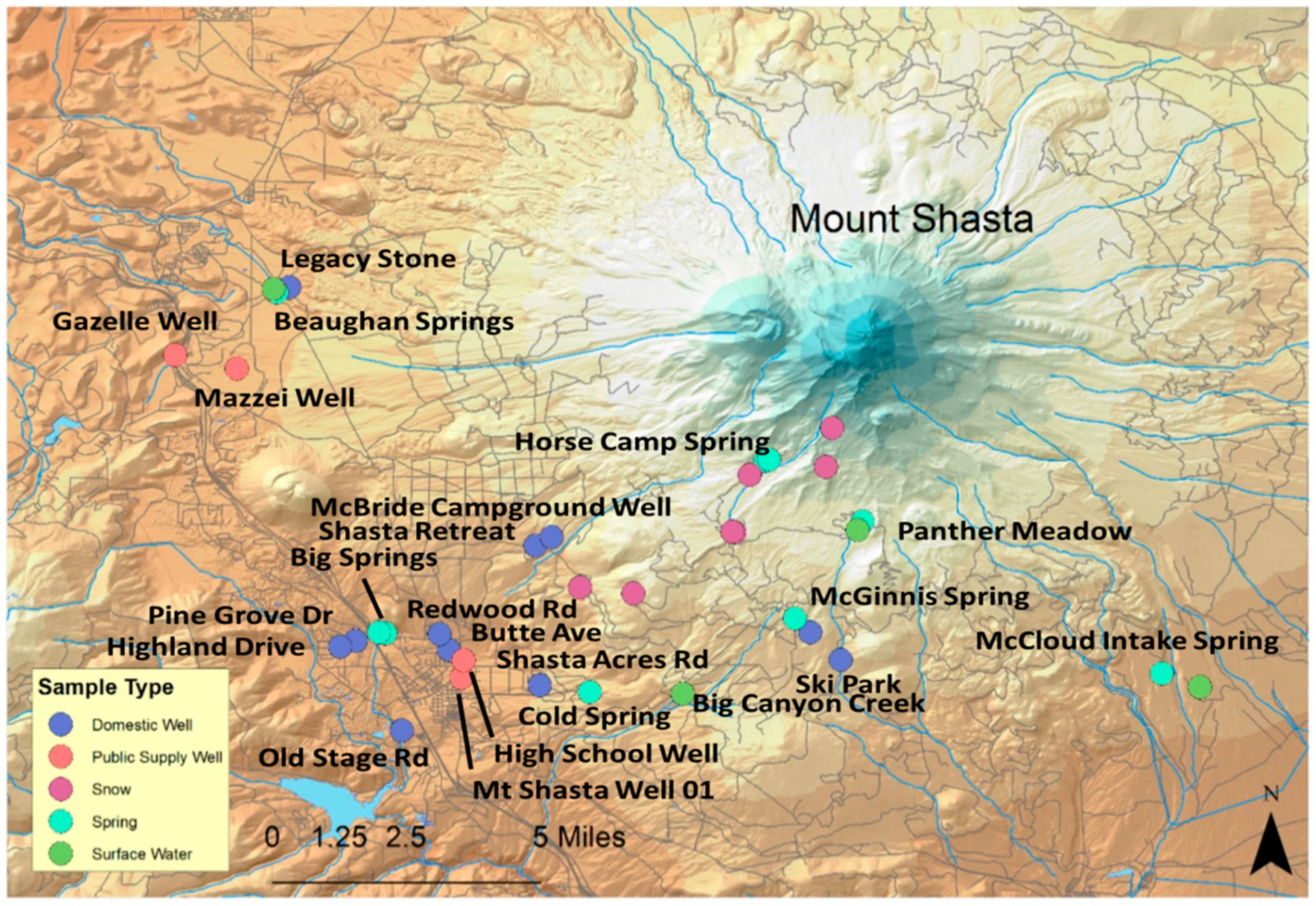
We sampled water from springs, domestic and water supply wells and streams in May and September 2015 (Table A1), during a period of extreme drought. Samples were collected from wells in the City of Weed, on the western flank of Mount Shasta; in the city of Mount Shasta, on the southwestern flank; and from wells and springs at higher elevations (Figure 1). All of the sampled springs are non-hydrothermal, or ‘cold’ springs. Snow samples (grab samples from just below the snow-air interface) were collected from the slopes of Mt Shasta between 1500 m and 3100 m elevation in February 2016.
Samples were collected from the sample port of public supply wells or spigots of domestic wells. Water samples from springs were collected from tubing connected to an outflow port when one was available. Dissolved oxygen (DO), conductivity, temperature, pH and oxidation-reduction potential (ORP) were measured at each location with a Thermo Orion Star A329 multi-meter (Table A1).
Stable isotopes of water were collected in 30 mL glass bottles and analyzed on a Los Gatos Research DLT-11 liquid water isotope analyzer (Los Gatos Research, Inc., San Jose, CA, USA) at California State University East Bay or on an isotope ratio mass spectrometer at Lawrence Livermore National Laboratory (LLNL). The same working standards (based on Vienna Standard Mean Ocean Water (VSMOW)) were used in both methods and a subset of samples was analyzed on both analyzers by way of intercomparison. One sigma uncertainties are within 1‰ for δ2H and 0.3‰ for δ18O. Tritium samples were collected in 1L Pyrex bottles and analyses were performed at LLNL by helium-3 accumulation [18,19] with a detection limit of 1 pCi/L (0.3 TU) and typical accuracy of 5%.
δ18O records a signature of surface air temperature and moisture source area, which is controlled by physiographic effects such as orographic lifting and distance inland in California [20]. The topographic relief of Mt Shasta, with its lapse rate in temperature and orographic precipitation, imparts a gradient in stable isotope signatures, known as the ‘altitude effect’ [21]. A lapse rate of −2‰ per 1000 m of elevation gain was first observed in precipitation samples from temperate regions and was attributed to the temperature dependence of isotopic fractionation during the condensation process [21]. Previous work based on observed δ18O in small springs and creeks (assumed to represent average meteoric water near the sampling locations) along a transect from low to high elevation in the Hat Creek Basin, 100 km (62 miles) to the southeast of Mt Shasta, indicates a lapse rate for δ18O of −2.3‰ per 1000 m increase in elevation [14]. Another set of observations within the Cascade Range showed a lapse rate of −1.4‰ per 1000 m [15].
Dissolved gas samples were collected to avoid atmospheric contamination by pressure tanks at well sites, or by entrainment of ambient air while vessels were filled. Noble gas and helium isotope samples were collected in 10 mL crimped copper tubes and were analyzed at the LLNL noble gas mass spectrometry facility [22,23,24]. Measurement uncertainty is 2% for the helium isotope ratio and dissolved concentrations of helium, neon and argon and is 3% for krypton and xenon concentrations. Noble gas concentrations for six samples were collected in VOA vials with no headspace and analyzed on a noble gas membrane inlet mass spectrometer (NG-MIMS) [25]. This method was used for spring locations where it was not possible to use the copper tube sampling method.
Noble gas derived parameters (recharge temperature/recharge elevation, excess air, terrigenic helium-4, terrigenic helium isotope ratio and tritiogenic helium-3) were calculated using the unfractionated excess air (UA) model [26]. This simplest excess air model was used in order to avoid bias in derived parameters resulting from the choice of the excess air model [23,25]. Data reduction followed the methods described in [27].
Patterns in dissolved noble gas concentrations in groundwater samples (Table A2) provide an independent method for examining recharge elevations. The dissolved concentration of noble gases in water is a function of temperature, air pressure (controlled by altitude) and salinity (negligibly small in the study area). Because of their conservative behavior in groundwater, the concentration of noble gases, especially the heavier gases whose solubilities have the strongest temperature dependency, can be used to deduce groundwater recharge temperature [28]. After measured noble gas concentrations are corrected for ‘excess air’ [26], recharge temperatures are typically calculated using an assumed pressure (often the atmospheric pressure at the elevation of the wellhead) and equilibrium solubility relationships [27]. However, because of the strong correlation between temperature and pressure in mountainous settings, calculated temperatures are non-unique and a range of plausible values, constrained by the physical conditions of the setting, must be considered [29,30,31].
For our samples, the maximum possible recharge elevation is the highest elevation on the mountain (4300 m), while the minimum recharge elevation is the sample discharge elevation. Similarly, the minimum recharge temperature is 0 °C, while the maximum recharge temperature is the discharge temperature. Applying these constraints, noble gas recharge temperatures were calculated at a range of elevations from the highest possible elevation or lowest possible temperature (0 °C), to the lowest elevation or highest temperature (Table A2).
2.2. Spatial Analysis
The local topography and meteorology result in strong differences between the windward (south west) and leeward (north east) side of Mt Shasta in terms of land cover, precipitation and temperature. In support of the interpretation of the isotopic and chemical data, a spatial analysis was performed using publically available datasets of land cover (2011 National Land Cover Database) [32], precipitation and temperature (PRISM Climate Group, Oregon State University, http://prism.oregonstate.edu) and vegetation index (MODIS NDVI Data) [33]. The purpose of the spatial analysis was to examine land cover in recharge source areas and compare elements of the water budget for the study area. Analyses were carried out over a wedge-shaped area with a radius of 14 km (approximately the distance from the summit to the furthest wells), which contains all analyzed wells except Beaughan Spring and Legacy Stone.
PRISM (parameter-elevation relationships on independent slopes model) 30 year (1981–2010) mean monthly average precipitation data are used to estimate precipitation in the study area. PRISM data are calculated from a local climate-elevation regression function for each grid cell on a digital elevation model [34]. Stations are assigned weights based on the physiographic similarity of the station to the grid cell. Factors include distance, elevation, coastal proximity, topographic facet orientation, vertical atmospheric layer, topographic position and orographic effectiveness of the terrain.
Various methods for quantifying ET were considered, including empirical relationships such as Penman-Monteith and use of reference evapotranspiration (Eto) data from CIMIS (California Irrigation Management Information System; www.cimis.water.ca.gov) [35]. CIMIS, which uses weather data to determine average daily Eto for short grass, shows ET for this section of Mount Shasta ranging from 2.35 to 3.39 mm/day, or 858 to 1237 mm/year. As an alternative more appropriate for a mountainous region with conifer forests, we use the relationship described in Goulden and Bales (2014) [10] for watersheds across the Sierra Nevada, which they applied to estimate ET from normal difference vegetation index (NDVI) data (measured by the Moderate Resolution Imaging Spectroradiometer (MODIS) Aqua satellite and averaged for snow- and cloud-free periods). ET is calculated using the following regression between annual average NDVI and annual ET [10]:
High resolution (~10 m) land cover data (National Land Cover Dataset obtained from the Multi-Resolution Land Characteristic Consortium, www.mrlc.gov) [36,32] was analyzed for the wedge in the southwestern quadrant of Mt Shasta. Land cover data for 2011 were obtained for each 250 m contour section within the wedge and ET was calculated from Equation (1) for each NDVI grid cell and averaged over each 250 m contour interval.
2.3. Flow Path Analysis
Relationships between recharge temperature and discharge temperature contain information about groundwater flow paths. Water moving through the subsurface transports heat and changes the subsurface temperature distribution. The rate of change of thermal energy in a parcel of groundwater is the sum of gravitational potential energy dissipation, heat transfer to/from the surface and geothermal heating [37]. In the case of Mount Shasta aquifers, conductive heat transport to/from the surface can be ignored because the advective rate of heat transport due to groundwater flow in the permeable aquifer materials is much greater than the rate of conductive heat transport. Using the elevation difference between recharge and discharge, as indicated by δ18O and noble gas recharge temperature analysis, the potential energy dissipation (gravitational) term can be calculated and subtracted from the total energy change to reveal the geothermal heating component. Geothermal gradients are strongly affected by shallow groundwater circulation in the Cascade Range [38], with shallow gradients as low as 15 °C/km but deeper gradients, which are affected by magma bodies, consistently >60 °C/km.
Comparison of the activity of tritium (pCi/L) of a water sample with the activity of a snow sample (taken within the same watershed or recharge area) allows determination of an approximate apparent groundwater age. The following version of the decay equation is used to calculate the apparent groundwater age (t) in years, using a 3H half-life of 12.32 years (decay constant of 0.056):
3H is the activity of the water sample and 3H0 is the activity of a snow sample, which is taken to represent the initial 3H activity.
Mean apparent groundwater residence times can be calculated from the parent-daughter pair, tritium and tritiogenic 3He [39]. However, separating tritiogenic 3He from the other components of helium present in groundwater is challenging in volcanic settings, where magmatic fluids mix with meteoric water [40]. Terrigenic helium was detected in a few of the well samples in the study area, along with magmatic helium in some cases (Table A2). Here, we use a relatively simple analysis of tritium to estimate a model groundwater ‘age.’
3. Results
3.1. Recharge Source Area
3.1.1. Stable Isotopes of Water
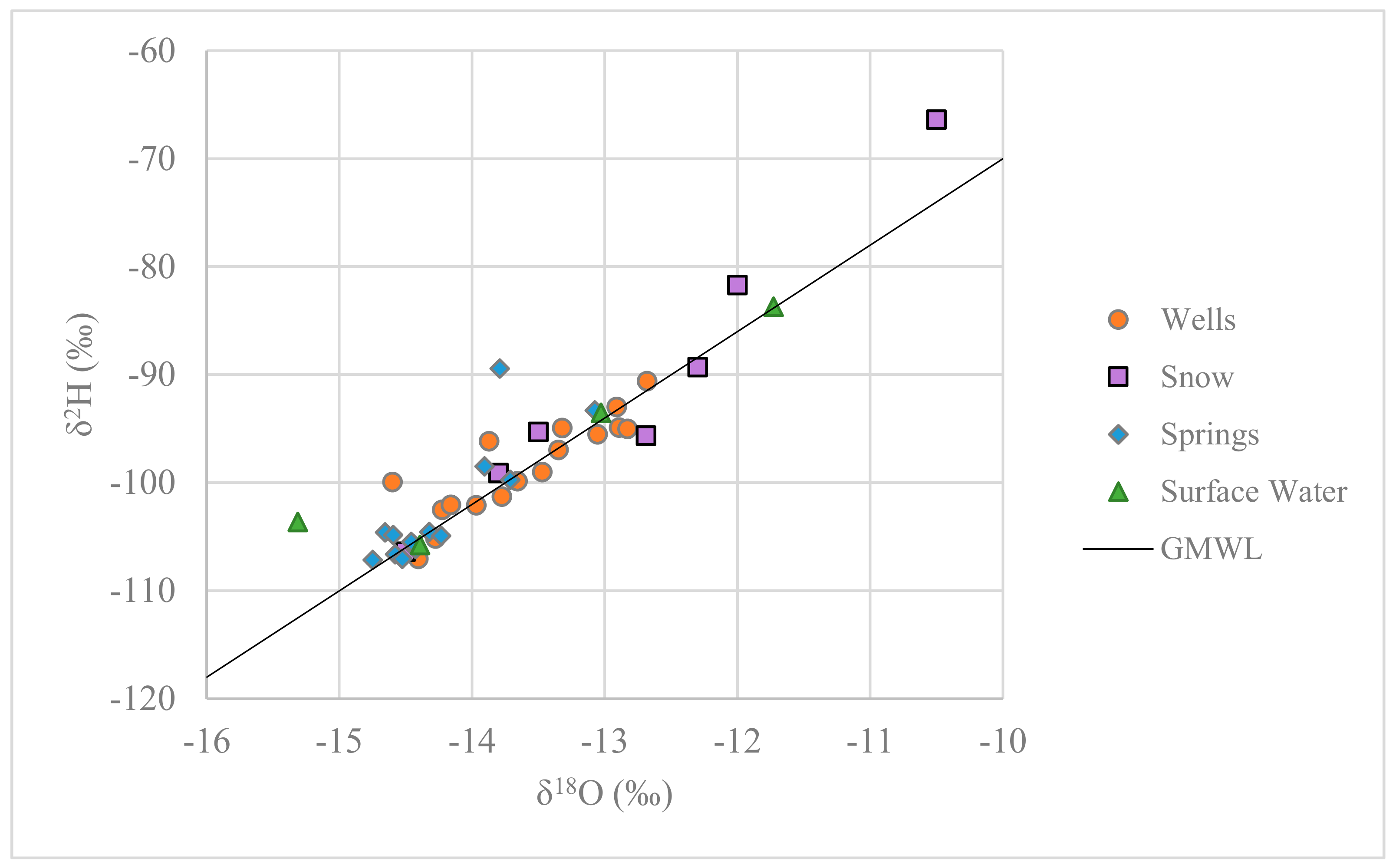
Our results for δ18O in snow samples retrieved from elevations between approximately 1900 m and 3100 m indicate a lapse rate of −2.1‰ per 1000 m (R2 = 0.96), in close agreement with the −2.3‰ per 1000 m determined by Rose et al. (1996) [14]. The consistency in lapse rates suggest that the effects of variation in the origin and path of storm tracks is negligible compared to the orogenic/elevation effect and that in this setting, on the windward side of Mt Shasta, stable isotopes are faithful indicators of the elevation at which precipitation (mainly snow), was deposited. The snow samples and nearly all other samples, fall on or near the global meteoric water line (Figure 2).
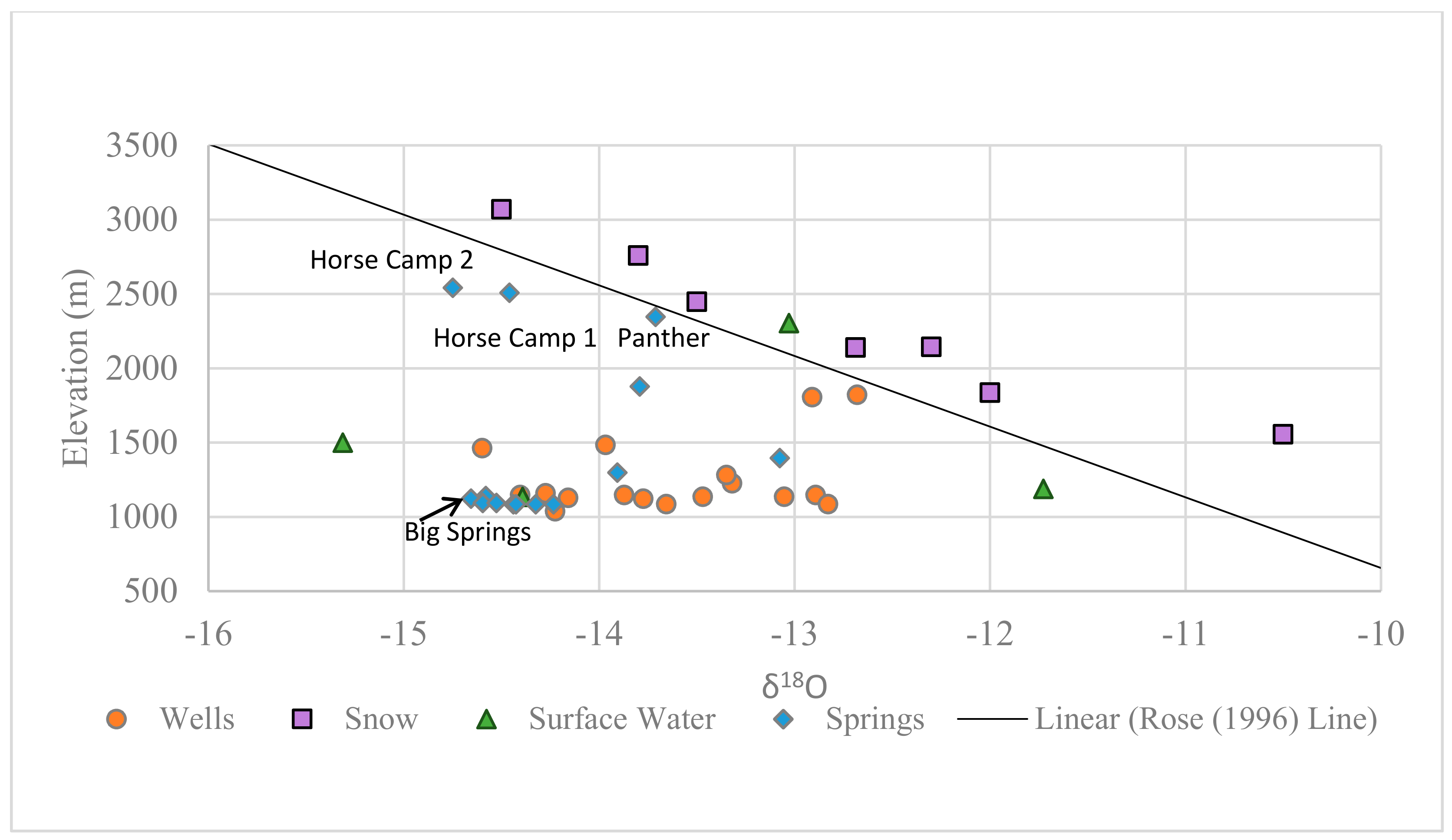
Many spring and groundwater samples from approximately 1000–1400 m elevation have δ18O values that fall well below the lapse rate trend line (Figure 3) indicating that groundwater from these locations is sourced from much higher elevations. Considering the elevations indicated by the lapse rate, the water source elevations for all of the springs and wells sampled fall between approximately 2000 and 2900 m. The elevation range over which springs recharge is somewhat higher (2500–2900 m) than the range for wells (2000–2700 m). The largest disparity between the sample elevation and the recharge elevation indicated by the δ18O lapse rate is for Big Springs, where a difference between recharge and discharge elevations of nearly 1700 m is indicated. In contrast, high elevation springs (Horse Camp 1, Horse Camp 2, Panther) show recharge elevations only slightly higher than sample elevations. Based on the lapse rate, the extrapolated δ18O value of precipitation from the summit of Mount Shasta (4322 m) would be −17.3‰, while precipitation from elevations below 2000 m is predicted to be greater than −12.3‰. The absence of samples with estimated recharge elevations above 2900 m or below 2000 m is an indication that the δ18O values could represent a mixture of water from both higher and lower elevations. This possibility is explored further in the Discussion section.
3.1.2. Noble Gas Recharge Conditions
Noble gas recharge temperatures were calculated for a range of possible recharge elevations, from the well elevation to the highest elevation on the mountain, resulting in a recharge temperature above 0 °C, as described in Section 2 (Table A2). The resulting ranges of possible recharge temperatures for each sample (represented as parallel lines calculated for each sample on Figure 4) have a slope equivalent to 2 °C per kilometer of elevation. The atmospheric lapse rate further constrains the recharge elevation for these samples and the elevation at which the line for each sample intersects the atmospheric lapse rate line is a plausible estimate of the recharge elevation (Figure 4). The atmospheric lapse rate was derived from a regression of mean annual air temperature data for each PRISM pixel on the study area quadrant and the mean annual air temperature was calculated as a function of elevation z (in km): 18.1 °C − z × 6.0 °C/km. The estimated recharge elevation of most samples lies between 2100 m and 2900 m. Two sample lines do not intersect with the local lapse-rate—Horse Camp 1 and 2. These samples were collected in VOAs, from small pools when the ambient air temperature was high (September) and may have (at least partially) re-equilibrated at the higher temperature, or may reflect summertime recharge only. Two wells (Highland Dr and Pine Grove Dr) on the western-most part of the study area have chemical and radiogenic helium signatures different from all other samples (Table A2), indicating that they likely recharge in the Klamath Mountains to the west and not on Mt Shasta. These two results are not included in the likely recharge elevation range.
3.1.3. Spatial Analysis
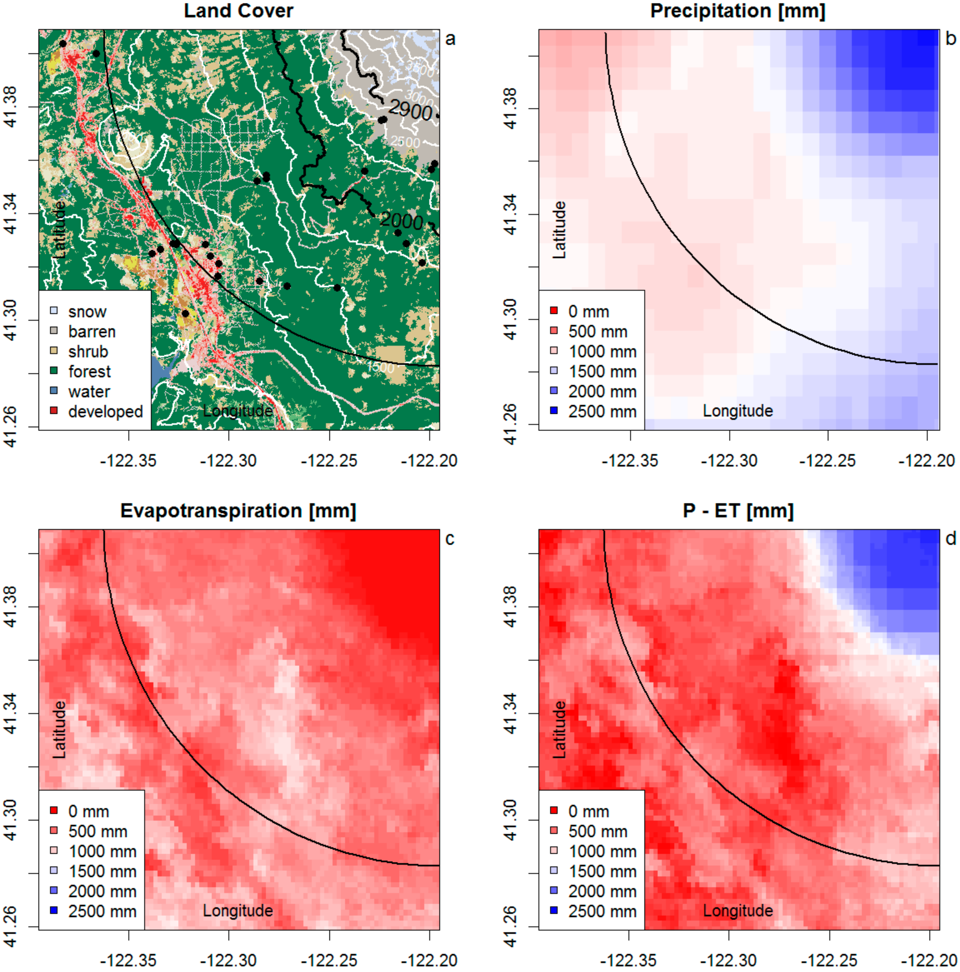
Elevation within the sector of radius 14 km (southwestern quadrant) of Mt Shasta varies between 1100 m and 4322 m. According to PRISM data, Mount Shasta has a precipitation low of 1112 mm/year, at the low elevation, western edge of the study area and a high of 2395 mm/year near the peak of the mountain (Figure 5b). The average precipitation rate within each 250 m contour section within the wedge was estimated and weighted according to the fractional area of each contour section over the entire wedge area (Table A4). Over that range, mean annual air temperature decreases from 11 °C to −7 °C. The groundwater recharge elevation band indicated by stable isotope and recharge temperature results is highlighted in Figure 5a by black contours at 2000 m and 2900 m.
Evapotranspiration estimates (based on Equation (1)) vary from approximately 700 mm/year at the base of the mountain to slightly over 100 mm/year above 2750 m. The strong decrease in ET around 2500 m coincides with the transition from forest to barren land (Figure 5a,c). The difference between precipitation and evapotranspiration (P−ET) is available for groundwater recharge and runoff. Very few surface water features exist on Mt Shasta and P−ET mainly infiltrates the permeable slopes. The combined patterns of P and ET (Figure 5d) result in a strong contrast of high water availability (blue) above 2500 m and low water availability (red) below 2000 m.
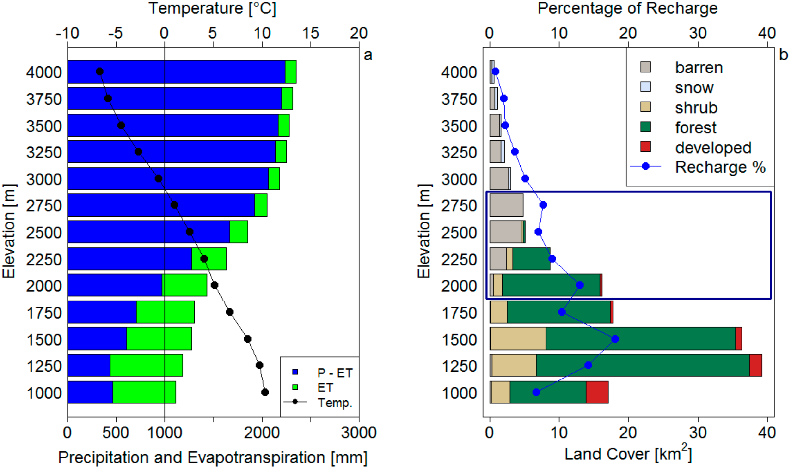
A bar graph of precipitation and ET (Figure 6a) shows that below 2000 m, about 60% of precipitation is lost to evapotranspiration, while less than 10% is lost above 2500 m. Net recharge (P−ET) rates increase from 550 mm below 1500 m to 1000 mm at 2000 m and 2000 mm above 3000 m. Because of the large proportion of land area at lower elevations, the average P−ET is 800 mm.
Below 2250 m elevation, forest (dark green on Figure 6b) is the dominant land cover. Between 2250 m and 2500 m elevation, forest is replaced by barren soil (gray on Figure 6b) and increasingly above 3000 m by perennial snow (light blue on Figure 6b). Despite the large proportion of barren land above 2500 m, the total area of barren land is limited, because the total surface area quickly decreases with increasing elevation. The blue box in Figure 6b outlines the elevation range of recharge to the wells derived from stable isotopes and noble gas results. Within this range, forest occupies 57% of land area and barren land 35%. Including the entire elevation range above 2000 m (assuming that higher elevation recharge also contributes) the ratios change to 46% and 44% respectively.
Taking land area into account, it becomes clear that lower elevation bands contribute a larger percentage to total groundwater recharge. Within the 14 km radius, 70% of the land area is below 2000 m and less than 6% of the area is above 3000 m. The distribution of total precipitation is comparable (63% below 2000 m and 9% above 3000 m). Groundwater recharge (estimated as the difference between total precipitation and evapotranspiration) is shifted to higher elevations because of the higher precipitation and lower evapotranspiration rates at higher elevations (48% below 2000 m and 15% above 3000 m). This is expressed by the differences between the percentage of recharge and the total land cover in Figure 6b. The contribution to recharge from each elevation band above 2500 m is higher than the total land area. Below 2000 m, the contribution of recharge is lower than the land area, especially below 1500 m. It is surprising that while all samples indicate a recharge elevation between 2000 m and 2900 m, more than 50% of recharge is estimated (through spatial analysis) to occur below 2000 m or above 3000 m. It is possible that this first approximation of recharge contributions on Mt Shasta underestimates evapotranspiration from forest at lower elevations and thereby overestimates recharge contributions at lower recharge elevations. The upper range of recharge elevations (2900 m) coincides with the elevation at which the mean annual air temperature is 0 °C.
3.2. Groundwater Flow Paths
3.2.1. Temperature Changes between Recharge and Discharge
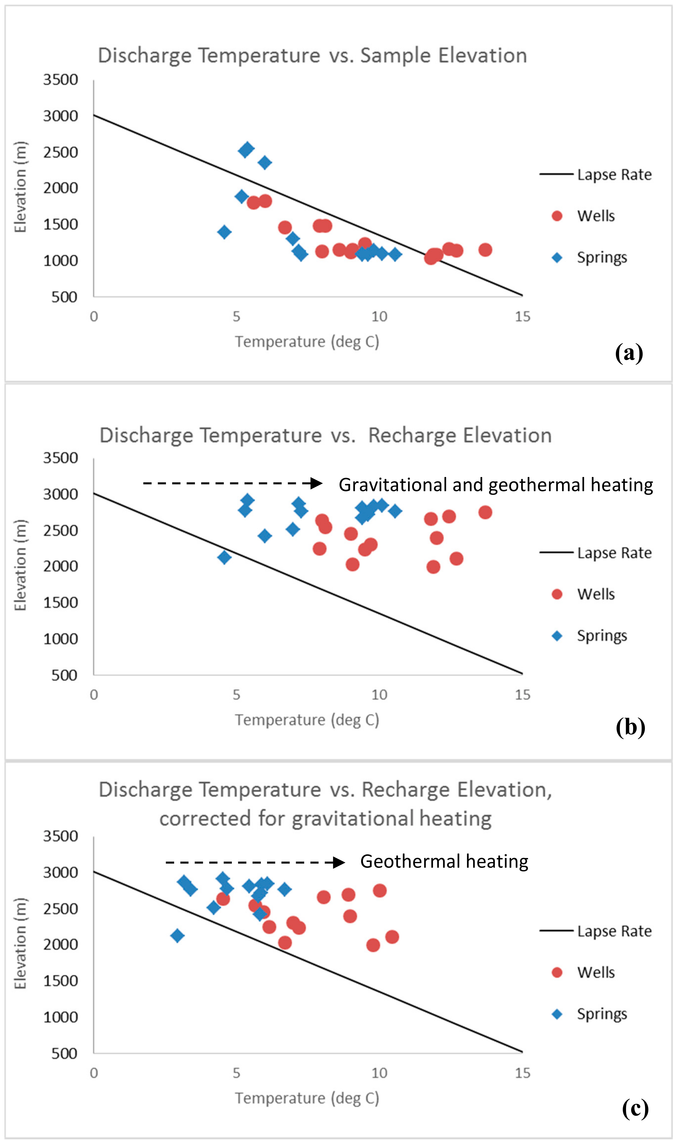
Discharge temperatures are plotted against elevation for wells and springs, along with the expected lapse rate of temperature vs. elevation in Figure 7a. Most samples plot below the line, i.e., discharge temperatures are colder than the predicted ambient air temperature. Panther Spring, Horse Camp 1 and Horse Camp 2, which have discharge temperatures of 5–6 degrees C, were sampled in September in pools, so they were likely warmed due to the higher summer air temperatures. In contrast, three wells that plot above the lapse rate at 13–14 degrees C may be influenced by deep flow paths and geothermal heating.
When discharge temperature is plotted against δ18O recharge elevation (available for all samples; Figure 7b), nearly all samples plot well above the lapse rate trend, i.e., discharge temperatures are higher than recharge temperatures. Figure 7c corrects for heating by gravitational energy accumulated along downslope flow paths. Figure 7c indicates that well samples, especially, show evidence for several degrees of geothermal heating during transport. The fact that well samples show greater geothermal heating than springs is likely due to deeper groundwater flow paths for at least a portion of the produced well water. For samples with e.g., 8 °C of geothermal heating and assuming a geothermal gradient at the low end of the observed range (15 °C/km), a maximum groundwater flow depth of about 500 m is indicated by this analysis.
Using the estimated recharge elevations, discharge locations and maximum flow depths, conceptual groundwater flow paths for each sample can be delineated. Three example flow paths are shown on Figure 8. Recharge locations and flow depths are averaged and approximate; however, these flow paths highlight the differences between the long, deep flow paths to the Mt. Shasta Big Springs and to wells on the lower slopes and the short, shallow flow paths to smaller, higher springs. These flow paths, based on geochemical and isotopic data, allow visualization of subsurface flow that is based on observational results rather than the flow paths typically depicted in groundwater studies, which are based on numerical models. Permeable, fractured, volcanic flow deposits are increasingly thick at lower elevations, so much of the subsurface residence time is likely accumulated at these lower elevations.
3.2.2. Groundwater Travel Times
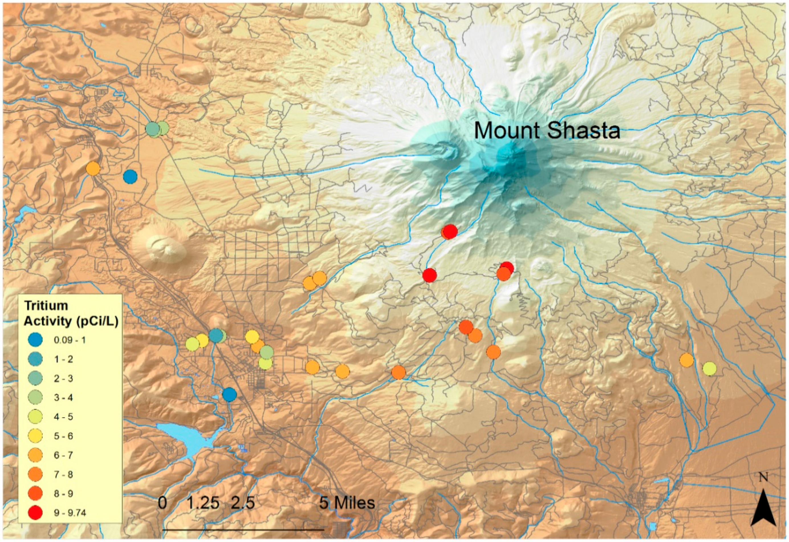
Tritium (half-life 12.3 years) was detected in all but two samples from the study area, so nearly all samples show evidence for (at least a component of) water with a residence time of less than approximately 50 years (Table A5). Tritium activity is affected by both spatial patterns in precipitation (with higher values expected for higher elevations [41] and by the decay of tritium during groundwater flow. Samples from higher elevations on Mount Shasta generally show higher tritium activity (red colors; Figure 9). Also, higher tritium activities are correlated with lower electrical conductivity, likely due to the fact that with increasing subsurface residence time, water-rock interaction contributes to increasing conductivity. Activities in lower elevation samples are lower and show more variability, which could be due to either the decay of tritium or lower initial activity, or both. Mixing of young and old groundwater during transport is also expected. For the simplest case, assuming ‘piston flow’ and an initial activity that matches the activity measured in snow at elevation 2140 m, Equation (2) is used to calculate mean, apparent ages. Results, shown in Table A5, reveal that water supply wells of the City of Mt Shasta (Well 01 and High School Well) produce water with a mean apparent age of 15–18 years, while Cold Spring, another important public water supply source, discharges younger water with a model age of 5 years. The high elevation springs on the slopes of Mt Shasta discharge groundwater that is recently recharged (0–5 years).
The Big Springs complex in the City of Mt Shasta has multiple discharge locations over a relatively small area, comprising large and small discharges totaling approximately 0.6 m3/s (20 cfs). Field parameters such as discharge temperature and EC differ significantly at the various discharge locations, suggesting discrete flow paths with differing water-rock interaction. Interestingly, however, δ18O values are not significantly different, suggesting similar recharge elevations. The tritium activity in the main spring outlet corresponds to 20 years of decay. Two other outlets have lower activities, which must be the result of mixing between modern and pre-modern groundwater, or discrete flow paths with differing travel times. The fourth sampled Big Springs outlet produced entirely pre-modern groundwater.
4. Discussion
The two independent tracer approaches to estimating the recharge elevation, δ18O and fitting the noble gas recharge temperature to the atmospheric lapse rate, agree remarkably well for the majority of the samples (Figure 10). Since stable isotopes are indicators of water source but not necessarily recharge elevation, the good agreement also suggests that water is not generally transported long distances overland before recharging. This conclusion is corroborated by observed high infiltration rates in permeable surface materials and a lack of continuous creeks and streams in the study area. As noted previously, two wells with noble gas-derived recharge temperatures that indicate recharge below 2000 m (Pine Grove Dr and Highland Dr) are located on the western edge of the study area and multiple lines of evidence (terrigenic helium, major ion and field chemistry) indicate this groundwater does not recharge on Mt Shasta. Three additional samples (Mazzei well, Beaughan Springs and Legacy Stone well) were sampled at the northern edge of the study area. For these wells, either the atmospheric lapse rate or the stable isotope trend could be different than the trend expected for the southwestern portion of Mount Shasta. The discrepancy for Shasta Acres Rd is unexplained. In summary, δ18O and noble gases are in close agreement and both indicate that the elevation range between 2000 m and 2900 m is most important for recharge.
Considering the elevation of the peak, an even greater range in δ18O might be expected, with even lighter (more negative) values than those observed, if any of the samples had source water entirely from elevations between 2900 m and 4300 m. The small area for accumulation of snow within the wedge considered (less than 6% of the land surface is above 3000 m elevation), comparable fraction of total precipitation (9% above 3000 m) and relatively long residence time of water in snow fields, are the likely explanations for the lack of δ18O observations that would indicate water sourced from very high elevations. The mean annual air temperature is close to 0 °C at 2900 m, so it is possible that higher elevation precipitation is not able to recharge to groundwater flow paths that reach the base and instead runs off superficially to recharge at lower elevations.
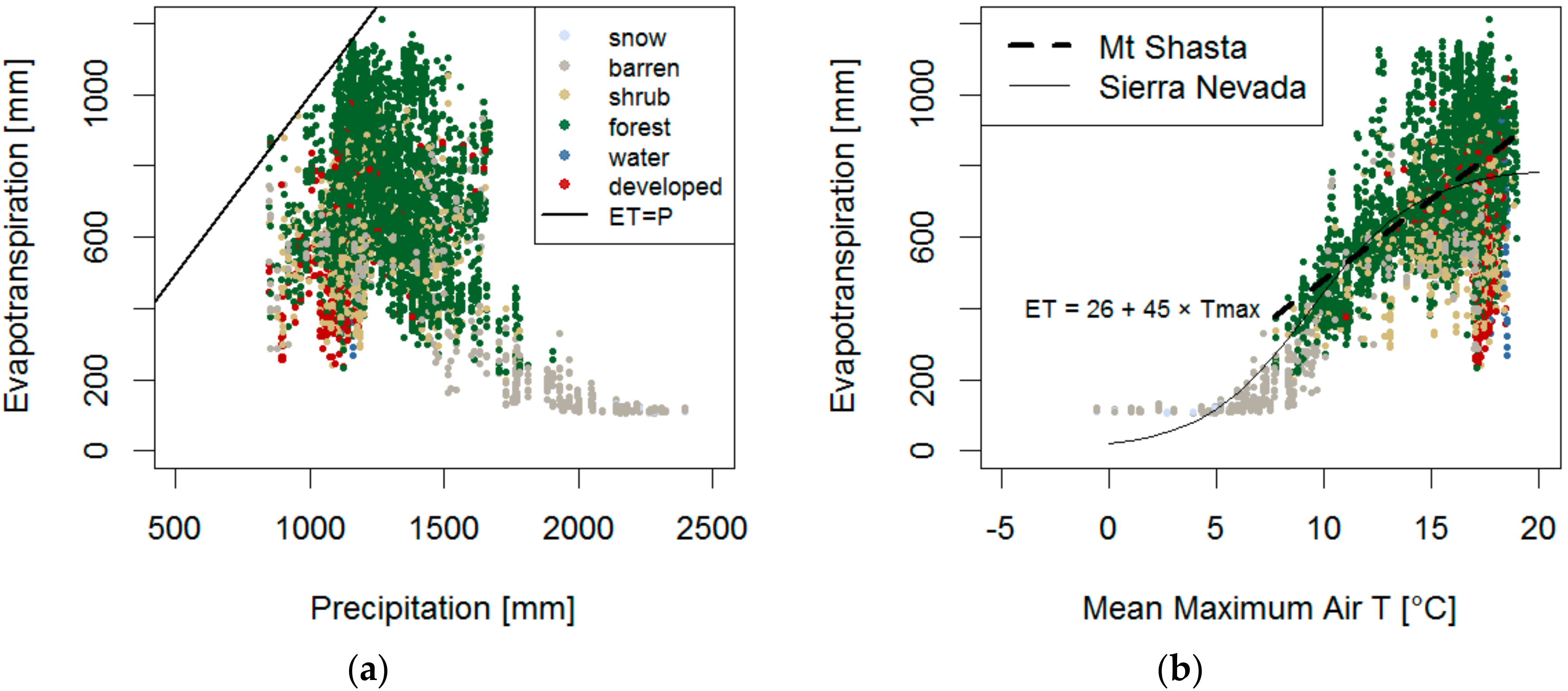
The lack of δ18O observations that would indicate water sourced from elevations between 1000 m and 2200 m is perhaps more surprising given that a large portion of the surface area (70%) and a comparable fraction of the total precipitation on the mountain, occur below 2200 m. However, ET increases sharply below 2400 m (Figure 6 and Table A4), with ET rates equivalent to roughly half of the precipitation rates. The lack of recharge from lower forest-covered elevations may therefore result from high evapotranspiration on forested slopes limiting water availability for recharge and point to an important role for barren land with limited evapotranspiration in controlling recharge on Mt Shasta. The loss of barren land on Mt Shasta to forest encroachment in a warming climate may therefore have a significant effect on recharge under future climate change conditions. On the other hand, an increase in the area of barren land that is free of snow cover for an extended time period could lead to an increase in recharge, offsetting to some degree the loss of recharge due to the increase in forest ET. This study’s finding that elevations above 2000 m are disproportionally important to groundwater recharge is consistent with observations in the Southern Sierra Critical Zone Observatory [10,42]. NDVI derived estimates of annual evapotranspiration are below annual PRISM precipitation suggesting evapotranspiration is not water limited (Figure 11a). For the Sierra Nevada, water limitation of evapotranspiration occurs only below 1000 mm annual precipitation [10].
We find a significant correlation between the NDVI derived annual evapotranspiration and the PRISM derived mean maximum annual air temperature (R2 = 0.38, p < 0.001) for forest land cover (Figure 11b). The slope of the regression (45.4 ± 0.9 mm/°C) implies an increase of 90 mm for a 2 °C warming scenario. The Mt Shasta linear regression is similar to the sigmoidal regression found by Goulden and Bales (2014) [10] for the Sierra Nevada (Figure 11b). Without forest encroachment, we predict that this increase in forest evapotranspiration will lead to a 7% decrease of net recharge (P−ET) for the southwest quadrant of Mt Shasta. Tree encroachment will have a delayed effect and further reduce P−ET. ET is strongly affected by both temperature and vegetation cover. An upslope shift in forest cover is expected if temperature is the primary control on vegetation. Likewise, an extended period of time above freezing and more water in shallow soils at high elevations allows seeds to sprout, leading to an upslope shift. Although decreased overland flow would be a typical outcome of increased forest cover, the highly permeable surface materials in this setting already largely preclude this process. The loss of barren land over the elevation range 2300–2900 m on Mt Shasta to forest encroachment in a warming climate would therefore have a significant effect on recharge under future climate conditions. However, in a study of tree line elevation change in alpine and subalpine settings, Hoch and Korner [43] found that the tree line moved upslope in only half of the 166 study locations, so although upslope movement of the tree line is an intuitive outcome of warmer conditions, the interactions between climate, forest habitat and ET are complex and difficult to predict. Observation and prediction of movement of the tree line on Mount Shasta will be important for predicting future changes in the hydrologic system, considering the importance of recharge at elevations just above the tree line.
The long, deep flow paths to the main wells and springs tapped for municipal and industrial supply, which result in subsurface residence times of a decade or more, indicate that changes in recharge patterns will only be observed at discharge locations after a similar decadal time period. For discharge points having shorter flow paths and residence times, earlier melting and decreased recharge will have a more immediate effect and will likely lead to lower discharge and earlier cessation of late summer baseflow.
Acknowledgments
This work performed under the auspices of the U.S. Department of Energy by Lawrence Livermore National Laboratory under Contract DE-AC52-07NA27344. The study was funded by the California State Water Resources Control Board Groundwater Ambient Monitoring and Assessment Program. Special thanks to Meadow Fitton, who was a great source of knowledge on the local hydrologic conditions and whose enthusiasm was contagious. The manuscript was improved by the suggestions of three anonymous reviewers.
Author Contributions
Elizabeth Peters, Ate Visser, Jean Moran and Bradley Esser conceived and designed the experiments; Elizabeth Peters, Ate Visser, Jean Moran and Bradley Esser carried out field work. Elizabeth Peters performed the sample analyses; Elizabeth Peters, Ate Visser and Jean Moran analyzed the data; Elizabeth Peters, Jean Moran and Ate Visser wrote the paper.
Conflicts of Interest
The authors declare no conflict of interest.
Appendix A. Data Tables

Table A1.
Field Parameters (NM = Not Measured; NA = Not Applicable).
| Site Name | Sample Date | Sample Time | Sample Type | Elevation (m) | GPS Latitude (Decimal °N) | GPS Longitude (Decimal °W) | Field Temp (°C) | Field Conductivity (uS/cm) | Field pH | Field DO (mg/L) | Field ORP (mV) |
|---|---|---|---|---|---|---|---|---|---|---|---|
| Old Stage Rd | 20150501 | 1650 | Domestic | 1036 | 41.3025 | −122.3219 | 11.8 | 121.6 | 7.22 | 9.5 | −12.6 |
| Big Springs Main | 20150428 | 1400 | Spring | 1085 | 41.3287 | −122.3265 | 7.3 | 166 | 6.5 | 12.3 | −55.2 |
| Big Springs B | 20150428 | 1630 | Spring | 1085 | 41.3287 | −122.3265 | 10.6 | 218 | NM | 11.7 | −27.2 |
| Big Springs C | 20150428 | 1645 | Spring | 1085 | 41.3287 | −122.3265 | 9.6 | 146 | NM | 11.4 | −23.2 |
| Big Springs D | 20150428 | 1725 | Spring | 1085 | 41.3287 | −122.3265 | 9.4 | 146 | NM | 11.0 | −1.7 |
| Big Springs 2 | 20150918 | 1000 | Spring | 1094 | 41.3290 | −122.3281 | 10.1 | 142.5 | NM | 4.1 | NM |
| Big Springs 3 | 20150918 | 1025 | Spring | 1094 | 41.3290 | −122.3281 | 9.4 | 131.4 | NM | 9.0 | NM |
| Big Springs Pool | 20150918 | 945 | Spring | 1123 | 41.3287 | −122.3264 | 7.2 | 88 | NM | 10.3 | NM |
| Pine Grove Dr | 20150428 | 1810 | Domestic | 1085 | 41.3267 | −122.3345 | 11.9 | 25.3 | NM | 10.2 | 1.2 |
| Highland Drive | 20150501 | 1540 | Domestic | 1085 | 41.3250 | −122.3386 | 12.0 | 162.8 | 6.8 | 8.3 | 11.4 |
| Mt Shasta Well 01 | 20150501 | 830 | Public Supply | 1122 | 41.3167 | −122.3058 | 9.0 | 96.21 | 6.98 | 7.7 | 1.3 |
| Mt Shasta High School Well | 20150501 | 1500 | Public Supply | 1128 | 41.3214 | −122.3053 | 8.0 | 81.4 | 7.2 | NM | 2.5 |
| Butte Ave | 20150428 | 1100 | Domestic | 1134 | 41.3243 | −122.3093 | 9.7 | 80 | NM | 14.0 | NM |
| Gazelle Well | 20150429 | 1340 | Public Supply | 1134 | 41.4038 | −122.3831 | 12.7 | 109 | NM | 11.4 | 11.4 |
| Beaughan Springs | 20150430 | 1000 | Spring | 1140 | 41.4207 | −122.3558 | 9.8 | 101.7 | 6.94 | 9.7 | NM |
| Redwood Rd | 20150428 | 1025 | Domestic | 1146 | 41.3284 | −122.3118 | 9.1 | 87 | 7.34 | 2.1 | −53.7 |
| Redwood Rd | 20150917 | 1445 | Domestic | 1146 | 41.3284 | −122.3118 | 8.6 | 10.16 | 7.01 | 11.0 | 5.1 |
| Legacy Stone Property | 20150430 | 1500 | Domestic | 1146 | 41.4220 | −122.3523 | 13.7 | 152.5 | 6.9 | 9.4 | 5.6 |
| Mazzei Well | 20150429 | 1410 | Public Supply | 1158 | 41.4001 | −122.3665 | 12.4 | 159 | NM | 8.9 | 41 |
| Shasta Acres Rd | 20150501 | 1430 | Domestic | 1225 | 41.3147 | −122.2847 | 9.5 | 87.22 | 7 | 9.7 | 0.2 |
| Mt Shasta Cold Spring | 20150501 | 1100 | Spring | 1298 | 41.3128 | −122.2712 | 7.0 | 42.04 | 6.92 | 10.1 | 4.4 |
| Shasta Retreat | 20150917 | 1830 | Domestic | 1461 | 41.3524 | −122.2859 | 6.7 | 65.66 | 6.57 | 8.4 | 30.1 |
| McBride Campground Well | 20150502 | 940 | Domestic | 1483 | 41.3546 | −122.2816 | 7.9 | 68.8 | 6.96 | 9.3 | 2.2 |
| McBride Campground Well | 20150917 | 1600 | Public Supply | 1483 | 41.3546 | −122.2816 | 8.1 | 68.35 | NM | 9.5 | NM |
| Ski Park 2 | 20150918 | 940 | Domestic | 1805 | 41.3290 | −122.2117 | 5.6 | 52.91 | 6.22 | 10.3 | NM |
| Ski Park 1 | 20150917 | 830 | Domestic | 1821 | 41.3216 | −122.2035 | 6.0 | 86.29 | 7.18 | 10.2 | −1.8 |
| McGinnis Spring | 20150917 | 1130 | Spring | 1878 | 41.3328 | −122.2159 | 5.2 | 56.07 | 6.95 | 9.6 | 9.3 |
| Panther Spring | 20150918 | 1230 | Spring | 2346 | 41.3589 | −122.1976 | 6.0 | 15.39 | NM | 9.5 | NM |
| Horse Camp Spring 1 | 20150918 | 1415 | Spring | 2509 | 41.3752 | −122.2239 | 5.3 | 13.51 | NM | 11.6 | NM |
| Horse Camp Spring 2 | 20150918 | 1500 | Spring | 2542 | 41.3755 | −122.2229 | 5.4 | 27.49 | NM | 10.8 | NM |
| McCloud Intake Spring | 20150429 | 845 | Spring | 1396 | 41.3179 | −122.1168 | 4.6 | NM | 7.2 | 14.1 | −16.2 |
| McCloud R at Lower Falls | 20150429 | 1050 | Surface Water | 1189 | 41.3142 | −122.1065 | 12.0 | 82 | NM | 11.9 | −30.8 |
| Panther Meadow Creek | 20150502 | 1210 | Surface Water | 2304 | 41.3566 | −122.1990 | 2.3 | 14.12 | 7.26 | 10.4 | −14.3 |
| Beaughan Creek at Roseberg Bridge | 20150430 | 1100 | Surface Water | 1134 | 41.4216 | −122.3565 | NM | NM | NM | NM | NM |
| Big Canyon Creek Middlefork | 20150917 | 1344 | Surface Water | 1500 | 41.3124 | −122.2461 | 5.6 | 49.76 | 6.71 | 11.4 | 22.5 |
| Bunny Flat snow | 20150502 | 1030 | Snow | 2140 | 41.3559 | −122.2322 | NA | NA | NA | NA | NA |
| Mt Shasta Snow 1 | 20160214 | Snow | 1554 | 41.3411 | −122.2739 | NA | NA | NA | NA | NA | |
| Mt Shasta Snow 2 | 20160214 | Snow | 1835 | 41.3394 | −122.2594 | NA | NA | NA | NA | NA | |
| Mt Shasta Snow 3 | 20160214 | Snow | 2143 | 41.3561 | −122.2328 | NA | NA | NA | NA | NA | |
| Mt Shasta Snow 4 | 20160214 | Snow | 2448 | 41.3714 | −122.2281 | NA | NA | NA | NA | NA | |
| Mt Shasta Snow 5 | 20160214 | Snow | 2758 | 41.3736 | −122.2075 | NA | NA | NA | NA | NA | |
| Mt Shasta Snow 6 | 20160214 | Snow | 3069 | 41.3842 | −122.2058 | NA | NA | NA | NA | NA |
Table A2.
Noble gas results.
| Site Name | 3He/ 4He | ± | 4He | ± | Ne | ± | Ar | ± | Kr | ± | Xe | ± | Pχ2 a | Recharge Temp. | 4HeTERb | RNA/Ra c |
|---|---|---|---|---|---|---|---|---|---|---|---|---|---|---|---|---|
| ×10−7 | ×10−8 cm3STP/g | ×10−8 cm3STP/g | ×10−5 cm3STP/g | ×10−8 cm3STP/g | ×10−9 cm3STP/g | % | °C | ×10−9 cm3STP/g | ||||||||
| Redwood Rd | 6.41 | 0.23 | 17.88 | 0.36 | 26.49 | 0.53 | 39.60 | 0.79 | 9.17 | 0.28 | 12.93 | 0.39 | 63% | 5.0 | 113.4 | 0.16 |
| Butte Ave | 19.88 | 0.32 | 5.07 | 0.10 | 21.84 | 0.44 | 37.95 | 0.76 | 8.75 | 0.26 | 12.91 | 0.39 | 49% | 4.2 | 0.0 | - |
| Pine Grove Dr | 4.33 | 0.08 | 62.47 | 1.25 | 19.88 | 0.52 | 35.97 | 0.72 | 8.47 | 0.25 | 12.09 | 0.36 | 58% | 7.2 | 578.0 | 0.26 |
| Gazelle Well | 16.33 | 0.27 | 4.61 | 0.09 | 20.06 | 0.40 | 36.53 | 0.73 | 8.57 | 0.26 | 12.52 | 0.38 | 58% | 5.4 | 0.0 | - |
| Mazzei Well | 69.82 | 1.14 | 26.62 | 0.53 | 20.56 | 0.41 | 36.76 | 0.74 | 8.74 | 0.26 | 12.75 | 0.38 | 67% | 4.6 | 217.9 | 5.94 |
| Beaughan Springs | 14.73 | 0.24 | 4.93 | 0.10 | 19.74 | 0.39 | 36.14 | 0.72 | 8.59 | 0.26 | 12.57 | 0.38 | 73% | 5.2 | 3.3 | 2.15 |
| Legacy Stone Property | 14.64 | 0.24 | 4.05 | 0.08 | 18.25 | 0.37 | 35.60 | 0.71 | 8.74 | 0.26 | 12.51 | 0.38 | 39% | 5.1 | 0.0 | - |
| Mt Shasta Well 01 | 58.75 | 0.96 | 12.80 | 0.26 | 22.22 | 0.44 | 38.12 | 0.76 | 8.99 | 0.27 | 13.34 | 0.40 | 73% | 2.6 | 75.3 | 6.53 |
| Mt Shasta Cold Spring | 13.23 | 0.22 | 4.15 | 0.08 | 18.93 | 0.38 | 37.36 | 0.75 | 8.89 | 0.27 | 13.36 | 0.40 | 33% | 1.9 | 0.0 | - |
| Mt Shasta High School Well | 26.81 | 0.24 | 5.40 | 0.11 | 20.19 | 0.40 | 37.40 | 0.75 | 9.09 | 0.27 | 13.26 | 0.40 | 40% | 2.5 | 7.1 | 8.26 |
| Shasta Acres Rd | 26.13 | 0.23 | 5.23 | 0.10 | 19.93 | 0.40 | 37.23 | 0.74 | 9.12 | 0.27 | 13.56 | 0.41 | 67% | 1.2 | 6.3 | 8.49 |
| Highland Drive | 5.91 | 0.17 | 129.32 | 2.59 | 19.17 | 0.38 | 33.86 | 0.68 | 8.25 | 0.25 | 11.87 | 0.36 | 74% | 8.1 | 1248.4 | 0.41 |
| Old Stage Rd | 77.24 | 0.69 | 20.37 | 0.41 | 22.23 | 0.44 | 40.40 | 0.81 | 9.52 | 0.29 | 13.63 | 0.41 | 2% | 1.4 | 151.1 | 7.18 |
| Ski Park 1 | 13.54 | 0.15 | 4.02 | 0.08 | 18.36 | 0.37 | 35.92 | 0.72 | 8.83 | 0.27 | 12.96 | 0.39 | 56% | 3.4 | 0.0 | - |
| Big Springs Pool | NC | NC | 5.00 | 0.25 | 22.66 | 1.13 | 38.36 | 0.77 | 9.08 | 0.18 | 13.79 | 0.28 | 96% | 0.7 | 0.0 | NC |
| Big Springs 2 | NC | NC | 5.83 | 0.29 | 22.89 | 1.14 | 37.96 | 0.76 | 8.90 | 0.18 | 13.52 | 0.27 | 96% | 2.0 | 3.7 | NC |
| Big Springs 3 | NC | NC | 6.39 | 0.32 | 23.48 | 1.17 | 38.74 | 0.77 | 8.99 | 0.18 | 13.89 | 0.28 | 83% | 0.5 | 7.8 | NC |
| Panther Spring | NC | NC | 4.21 | 0.21 | 20.97 | 1.05 | 35.97 | 0.72 | 8.62 | 0.17 | 13.19 | 0.26 | 75% | 2.9 | 0.0 | NC |
| Horse Camp Spring 1 | NC | NC | 4.22 | 0.21 | 20.65 | 1.03 | 34.70 | 0.69 | 8.21 | 0.16 | 12.25 | 0.24 | 58% | 6.7 | 0.0 | NC |
| Horse Camp Spring 2 | NC | NC | 4.01 | 0.20 | 19.49 | 0.97 | 33.52 | 0.67 | 8.07 | 0.16 | 11.71 | 0.23 | 56% | 9.0 | 0.0 | NC |
a Pχ2 (the chi-squared probability) is a measure for the goodness of fit for noble gas recharge temperatures that are modeled based on equilibrium solubility relationships for Ne, Ar, Kr and Xe (corrected for excess air component). b Terrigenic, or crustal 4He, due to the decay of U and Th, is calculated by subtracting equilibrium solubility and excess air components from the measured 4He. c The non-atmospheric 3He/4He ratio (RNA, non-atmospheric helium components), divided by the atmospheric 3He/4He ratio (Ra) is an indication of a magmatic He component. 6–8 Ra is common for magmatic He and values greater than 2 are indicative of a component of magmatic He. Values close to zero represent crustal helium from the decay of U and Th.
Table A3.
Stable isotope results.
| Site Name | SampleDate | Site Elevation (m) | δ18O SMOW (‰) | δD SMOW (‰) | δ18O Recharge Elevation (m) |
|---|---|---|---|---|---|
| Old Stage Rd | 20150501 | 1036 | −14.2 | −102.5 | 2665 |
| Pine Grove Dr | 20150428 | 1085 | −12.8 | −95.0 | 2001 |
| Highland Drive | 20150501 | 1085 | −13.7 | −99.9 | 2395 |
| Big Springs Main | 20150428 | 1085 | −14.4 | −105.7 | 2767 |
| Big Springs B | 20150428 | 1085 | −14.4 | −106.1 | 2761 |
| Big Springs C | 20150428 | 1085 | −14.3 | −104.5 | 2713 |
| Big Springs D | 20150428 | 1085 | −14.2 | −104.9 | 2669 |
| Big Springs Pool | 20150918 | 1123 | −14.7 | −104.6 | 2870 |
| Big Springs 2 | 20150918 | 1094 | −14.6 | −104.8 | 2841 |
| Big Springs 3 | 20150918 | 1094 | −14.5 | −107.0 | 2809 |
| Mt Shasta Well 01 | 20150501 | 1122 | −13.8 | −101.3 | 2451 |
| Mt Shasta High School Well | 20150501 | 1128 | −14.2 | −102.0 | 2633 |
| Butte Ave | 20150428 | 1134 | −13.5 | −99.0 | 2306 |
| Gazelle Well | 20150429 | 1134 | −13.1 | −95.5 | 2108 |
| Beaughan Springs | 20150430 | 1140 | −14.6 | −106.6 | 2834 |
| Redwood Rd | 20150428 | 1146 | −12.9 | −94.9 | 2031 |
| Redwood Rd | 20150917 | 1146 | −12.9 | −94.9 | 2031 |
| Legacy Stone Property | 20150430 | 1146 | −14.4 | −107.1 | 2750 |
| Mazzei Well | 20150429 | 1158 | −14.3 | −105.2 | 2689 |
| Shasta Acres Rd | 20150501 | 1225 | −13.3 | −95.0 | 2235 |
| Mt Shasta Cold Spring | 20150501 | 1298 | −13.9 | −98.5 | 2514 |
| McCloud Intake Spring | 20150429 | 1396 | −13.1 | −93.3 | 2119 |
| Shasta Retreat | 20150917 | 1461 | −14.6 | −99.7 | 2844 |
| McBride Campground Well | 20150502 | 1483 | −13.3 | −97.0 | 2248 |
| McBride Campground Well | 20150917 | 1483 | −14.0 | −102.1 | 2543 |
| Ski Park 2 | 20150918 | 1805 | −13.0 | −92.3 | 2083 |
| Ski Park 1 | 20150917 | 1821 | −12.9 | −93.9 | 2035 |
| McGinnis Spring | 20150917 | 1878 | −13.8 | −92.1 | 2463 |
| Panther Spring | 20150918 | 2346 | −13.7 | −99.7 | 2421 |
| Horse Camp Spring 1 | 20150918 | 2509 | −14.5 | −105.5 | 2777 |
| Horse Camp Spring 2 | 20150918 | 2542 | −14.7 | −107.1 | 2914 |
| McCloud R at Lower Falls | 20150429 | 920 | −11.7 | −83.7 | NA |
| Beaughan Creek at Roseberg Bridge | 20150430 | 1134 | −14.4 | −105.7 | NA |
| Panther Meadow Creek | 20150502 | 2304 | −13.0 | −93.5 | NA |
| Mt Shasta Snow 1 | 20160214 | 1554 | −10.5 | −66.4 | NA |
| Mt Shasta Snow 2 | 20160214 | 1835 | −12.0 | −81.7 | NA |
| Mt Shasta Snow 3 | 20160214 | 2143 | −12.3 | −89.3 | NA |
| Mt Shasta Snow 4 | 20160214 | 2448 | −13.5 | −93.5 | NA |
| Mt Shasta Snow 5 | 20160214 | 2758 | −13.8 | −99.1 | NA |
| Mt Shasta Snow 6 | 20160214 | 3069 | −14.5 | −106.4 | NA |
| Bunny Flat snow | 20150502 | 2140 | −12.9 | −97.3 | NA |
Table A4.
Results of Spatial Analysis.
| Elevation Range (m) | Area (%) | Distance to Summit (km) | Precipitation (mm) | P (%) | ET (mm) | ET (%) | P−ET (mm) | P−ET (%) | Temperature (°C) | Precipitation (mm) | ET (mm) | P−ET Norm |
|---|---|---|---|---|---|---|---|---|---|---|---|---|
| 1000–1250 | 11.1 | 13.2 | 1112 | 9% | 644 | 13% | 468 | 6% | 10.3 | 123.4 | 71.5 | 51.9 |
| 1250–1500 | 25.1 | 11.8 | 1190 | 22% | 746 | 33% | 444 | 14% | 9.7 | 298.7 | 187.2 | 111.4 |
| 1500–1750 | 23.4 | 10.5 | 1281 | 22% | 673 | 28% | 608 | 18% | 8.5 | 299.8 | 157.5 | 142.3 |
| 1750–2000 | 11.6 | 8.3 | 1306 | 11% | 596 | 12% | 710 | 10% | 6.7 | 151.5 | 69.1 | 82.4 |
| 2000–2250 | 10.5 | 6.9 | 1431 | 11% | 464 | 9% | 967 | 13% | 5.1 | 150.3 | 48.7 | 101.5 |
| 2250–2500 | 5.8 | 5.5 | 1629 | 7% | 351 | 4% | 1278 | 9% | 4.1 | 94.5 | 20.4 | 74.1 |
| 2500–2750 | 3.4 | 4.5 | 1853 | 5% | 181 | 1% | 1672 | 7% | 2.6 | 63.0 | 6.2 | 56.8 |
| 2750–3000 | 3.2 | 3.7 | 2050 | 5% | 130 | 1% | 1920 | 8% | 1 | 65.6 | 4.2 | 61.4 |
| 3000–3250 | 2 | 3 | 2177 | 3% | 115 | 0% | 2062 | 5% | −0.7 | 43.5 | 2.3 | 41.2 |
| 3250–3500 | 1.5 | 2.4 | 2238 | 2% | 112 | 0% | 2126 | 4% | −2.6 | 33.6 | 1.7 | 31.9 |
| 3500–3750 | 1.1 | 1.9 | 2270 | 2% | 114 | 0% | 2156 | 3% | −4.4 | 25.0 | 1.3 | 23.7 |
| 3750–4000 | 0.8 | 1.2 | 2309 | 1% | 113 | 0% | 2196 | 2% | −5.8 | 18.5 | 0.9 | 17.6 |
| >4000 | 0.4 | 0.6 | 2352 | 1% | 112 | 0% | 2240 | 1% | −6.9 | 9.4 | 0.4 | 9.0 |
Table A5.
Tritium and Model Age results.
| Site Name | 3H (pCi/L) | +/− (pCi/L) | Model Age (Year) |
|---|---|---|---|
| Old Stage Rd | 0.09 | 0.16 | >50 |
| Big Springs Main | 3.03 | 0.29 | 19.4 |
| Big Springs B | 1.05 | 0.22 | 38.3 |
| Big Springs C | 1.22 | 0.22 | 35.6 |
| Big Springs D | 0.17 | 0.75 | >50 |
| Big Springs Pool | 3.32 | 0.19 | 17.8 |
| Big Springs 2 | 1.33 | 0.13 | 34.0 |
| Big Springs 3 | 1.25 | 0.12 | 35.2 |
| Highland Drive | 4.56 | 0.32 | 12.2 |
| Pine Grove Dr | 5.81 | 0.35 | 7.9 |
| Mt Shasta Well 01 | 3.89 | 0.27 | 15.0 |
| Mt Shasta High School Well | 3.21 | 0.24 | 18.4 |
| Butte Ave | 6.45 | 0.50 | 6.0 |
| Gazelle Well | 6.50 | 0.42 | 5.9 |
| Beaughan Springs | 3.25 | 0.26 | 18.2 |
| Legacy Stone Property | 3.80 | 0.27 | 15.4 |
| Redwood Rd (April) | 4.94 | 0.52 | 10.8 |
| Redwood Rd (September) | 5.64 | 0.55 | 8.4 |
| Mazzei Well | 0.69 | 0.17 | >50 |
| Shasta Acres Rd | 6.65 | 0.55 | 5.5 |
| Mt Shasta Cold Spring | 6.81 | 0.46 | 5.1 |
| McCloud Intake Spring | 7.27 | 0.40 | 3.9 |
| Shasta Retreat | 6.57 | 0.54 | 5.7 |
| McBride Campground Well (May) | 6.02 | 0.15 | 7.2 |
| McBride Campground Well (September) | 6.33 | 0.96 | 6.4 |
| Big Canyon Creek Middlefork | 7.31 | 0.93 | 3.8 |
| Ski Park 2 | 7.96 | 0.60 | 2.3 |
| Ski Park 1 | 7.57 | 0.64 | 3.2 |
| McGinnis Spring | 8.57 | 0.63 | 1.0 |
| Panther Spring | 9.74 | 0.40 | −1.3 |
| Horse Camp Spring 1 | 8.78 | 0.37 | 0.5 |
| Horse Camp Spring 2 | 9.03 | 0.42 | 0.0 |
| Bunny Flat snow | 9.05 | 0.46 | 0.0 |
References
- López-Moreno, J.I.; Pomeroy, J.W.; Revuelto, J.; Vicente-Serrano, S.M. Response of snow processes to climate change: Spatial variability in a small basin in the spanish pyrenees. Hydrol. Process. 2013, 27, 2637–2650. [Google Scholar] [CrossRef]
- Hayhoe, K.; Cayan, D.; Field, C.B.; Frumhoff, P.C.; Maurer, E.P.; Miller, N.L.; Moser, S.C.; Schneider, S.H.; Cahill, K.N.; Cleland, E.E.; et al. Emissions pathways, climate change and impacts on California. PNAS 2004, 101, 12422–12427. [Google Scholar] [CrossRef] [PubMed]
- Mote, P.W.; Hamlet, A.F.; Clark, M.P.; Lettenmaier, D.P. Declining mountain snowpack in western North America. Bull. Am. Meteorol. Soc. 2005, 86, 39–49. [Google Scholar] [CrossRef]
- Fritze, H.; Stewart, I.T.; Pebesma, E. Shifts in western North American snowmelt runoff regimes for the recent warm decades. J. Hydrometeorol. 2011, 12, 989–1006. [Google Scholar] [CrossRef]
- Surfleet, C.G.; Tullos, D. Variability in Effect of Climate change on rain-on-snow peak flow events in a temperate climate. J. Hydrol. 2013, 479, 24–34. [Google Scholar] [CrossRef]
- Gershunov, A.; Shulgina, T.; Ralph, F.M.; Lavers, D.A.; Rutz, J.J. Assessing the climate-scale variability of atmospheric rivers affecting western North America. Geophys. Res. Lett. 2017, 44, 2017GL074175. [Google Scholar] [CrossRef]
- Polade, S.D.; Pierce, D.W.; Cayan, D.R.; Gershunov, A.; Dettinger, M.D. The key role of dry days in changing regional climate and precipitation regimes. Sci. Rep. 2014, 4. [Google Scholar] [CrossRef] [PubMed]
- Rapacciuolo, G.; Maher, S.P.; Schneider, A.C.; Hammond, T.T.; Jabis, M.D.; Walsh, R.E.; Iknayan, K.J.; Walden, G.K.; Oldfather, M.F.; Ackerly, D.D.; et al. Beyond a warming fingerprint: Individualistic biogeographic responses to heterogeneous climate change in California. Glob. Chang. Biol. 2014, 20, 2841–2855. [Google Scholar] [CrossRef] [PubMed]
- Sundqvist, M.K.; Sanders, N.J.; Wardle, D.A. Community and ecosystem responses to elevational gradients: Processes, mechanisms and insights for global change. Annu. Rev. Ecol. Evol. Syst. 2013, 44, 261–280. [Google Scholar] [CrossRef]
- Goulden, M.L.; Bales, R.C. Mountain runoff vulnerability to increased evapotranspiration with vegetation expansion. Proc. Natl. Acad. Sci. USA 2014, 111, 14071–14075. [Google Scholar] [CrossRef] [PubMed]
- Segal, D.C.; Moran, J.E.; Visser, A.; Singleton, M.J.; Esser, B.K. Seasonal variation of high elevation groundwater recharge as indicator of climate response. J. Hydrol. 2014, 519, 3129–3141. [Google Scholar] [CrossRef]
- Singleton, M.J.; Moran, J.E. Dissolved noble gas and isotopic tracers reveal vulnerability of groundwater in a small, high-elevation catchment to predicted climate changes: Vulnerability of high elevation groundwater. Water Resour. Res. 2010, 46. [Google Scholar] [CrossRef]
- Tague, C.; Grant, G.E. Groundwater dynamics mediate low-flow response to global warming in snow-dominated alpine regions. Water Resour. Res. 2009, 45, W07421. [Google Scholar] [CrossRef]
- Rose, T.P.; Lee Davisson, M.; Criss, R.E. Isotope hydrology of voluminous cold springs in fractured rock from an active volcanic region, northeastern California. J. Hydrol. 1996, 179, 207–236. [Google Scholar] [CrossRef]
- Nathenson, M.; Thompson, J.M.; White, L.D. Slightly thermal springs and non-thermal springs at Mount Shasta, California: Chemistry and recharge elevations. J. Volcanol. Geotherm. Res. 2003, 121, 137–153. [Google Scholar] [CrossRef]
- Jefferson, A.; Grant, G.; Rose, T. Influence of volcanic history on groundwater patterns on the west slope of the Oregon High Cascades. Water Resour. Res. 2006, 42, W12411. [Google Scholar] [CrossRef]
- Saar, M.O.; Manga, M. Depth dependence of permeability in the Oregon Cascades inferred from hydrogeologic, thermal, seismic and magmatic modeling constraints. J. Geophys. Res. 2004, 109, B04204. [Google Scholar] [CrossRef]
- Surano, K.; Hudson, G.; Failor, R.; Sims, J.; Holland, R.; MacLean, S.; Garrison, J. Heliuim-3 mass spectrometry for low-level tritium analysis of environmental samples. J. Radioanal. Nucl. Chem. 1992, 161, 443–453. [Google Scholar] [CrossRef]
- Clarke, W.B.; Jenkins, W.J.; Top, Z. Determination of tritium by mass spectrometric measurement of 3He. Int. J. Appl. Radiat. Isotopes 1976, 27, 515–522. [Google Scholar] [CrossRef]
- Dansgaard, W. Stable isotopes in precipitation. Tellus 1964, 16, 436–468. [Google Scholar] [CrossRef]
- Dansgaard, W. The Isotopic Composition of Natural Waters with Special Reference to the Greenland Ice Cap. Meddelelser Om GrÒ©Nland Vol 165 No 2; C. A. Reitzel: Copenhagen, Denmark, 1961. [Google Scholar]
- Rademacher, L.K.; Clark, J.F.; Hudson, G.B.; Erman, D.C.; Erman, N.A. Chemical evolution of shallow groundwater as recorded by Springs, Sagehen Basin; Nevada County, California. Chem. Geol. 2001, 179, 37–51. [Google Scholar] [CrossRef]
- Cey, B.D.; Hudson, G.B.; Moran, J.E.; Scanlon, B.R. Impact of artificial recharge on dissolved noble gases in groundwater in California. Environ. Sci. Technol. 2008, 42, 1017–1023. [Google Scholar] [CrossRef] [PubMed]
- Visser, A.; Singleton, M.J.; Hillegonds, D.J.; Velsko, C.A.; Moran, J.E.; Esser, B.K. A membrane inlet mass spectrometry system for noble gases at natural abundances in gas and water samples. Rapid Commun. Mass Spectrom. 2013, 27, 2472–2482. [Google Scholar] [CrossRef] [PubMed]
- Visser, A.; Fourré, E.; Barbecot, F.; Aquilina, L.; Labasque, T.; Vergnaud, V.; Esser, B.K. Intercomparison of tritium and noble gases analyses, 3H/3He ages and derived parameters excess air and recharge temperature. Appl. Geochem. 2014, 50 (Suppl. C), 130–141. [Google Scholar] [CrossRef]
- Heaton, T.H.E.; Vogel, J.C. “Excess Air” in groundwater. J. Hydrol. 1981, 50 (Suppl. C), 201–216. [Google Scholar] [CrossRef]
- Visser, A.; Moran, J.E.; Hillegonds, D.; Singleton, M.J.; Kulongoski, J.T.; Belitz, K.; Esser, B.K. Geostatistical analysis of tritium, groundwater age and other noble gas derived parameters in California. Water Res. 2016, 91, 314–330. [Google Scholar] [CrossRef] [PubMed]
- Aeschbach-Hertig, W.; Peeters, F.; Beyerle, U.; Kipfer, R. Palaeotemperature Reconstruction from noble gases in ground water taking into account equilibration with entrapped air. Nature 2000, 405, 1040–1044. [Google Scholar] [CrossRef] [PubMed]
- Manning, A.H.; Solomon, D.K. Using noble gases to investigate mountain-front recharge. J. Hydrol. 2003, 275, 194–207. [Google Scholar] [CrossRef]
- Cederberg, J.R.; Gardner, P.M.; Thiros, S.A. Hydrology of Northern Utah Valley, Utah County, Utah; 2008–5197; U.S. Geological Survey: Reston, VA, USA, 2009. [Google Scholar]
- Althaus, R.; Klump, S.; Onnis, A.; Kipfer, R.; Purtschert, R.; Stauffer, F.; Kinzelbach, W. Noble gas tracers for characterisation of flow dynamics and origin of groundwater: A Case study in Switzerland. J. Hydrol. 2009, 370, 64–72. [Google Scholar] [CrossRef]
- Homer, C.; Dewitz, J.; Yang, L.; Jin, S.; Danielson, P.; Xian, G.; Coulston, J.; Herold, N.; Wickham, J.; Megown, K. Completion of the 2011 National Land Cover Database for the Conterminous United States—Representing a Decade of Land Cover Change Information; American Society for Photogrammetry and Remote Sensing: Bethesda, MD, USA, 2015; Volume 81. [Google Scholar]
- Spruce, J.P.; Gasser, G.E.; Hargrove, W.W. MODIS NDVI Data, Smoothed and Gap-Filled, for the Conterminous US: 2000–2013; ORNL Distributed Active Archive Center: Oak Ridge, TN, USA, 2015. [Google Scholar]
- Stoklosa, J.; Daly, C.; Foster, S.D.; Ashcroft, M.; Warton, D. A Climate of uncertainty: accounting for error in climate variables for species distribution models. Methods Ecol. Evol. 2014, 6. [Google Scholar] [CrossRef]
- California Irrigation Management Information System. Available online: http://www.cimis.water.ca.gov/ (accessed on 30 October 2017).
- Multi-Resolution Land Characteristics Consortium (MRLC). Available online: https://www.mrlc.gov/ (accessed on 30 October 2017).
- Manga, M.; Kirchner, J.W. Interpreting the temperature of water at cold springs and the importance of gravitational potential energy. Water Resour. Res. 2004, 40, W05110. [Google Scholar] [CrossRef]
- Blackwell, D.D.; Steele, J.L.; Carter, L.C. Heat Flow Patterns of the North American Continent: A Discussion of the DNAG Geothermal Map of North America; DOEEEGTP (USDOE Office of Energy Efficiency and Renewable Energy Geothermal Tech Pgm): Washington, DC, USA, 1990. [Google Scholar]
- Schlosser, P.; Stute, M.; Dörr, H.; Sonntag, C.; Münnich, K.O. Tritium/3He dating of shallow groundwater. Earth Planet. Sci. Lett. 1988, 89, 353–362. [Google Scholar] [CrossRef]
- Saar, M.O.; Castro, M.C.; Hall, C.M.; Manga, M.; Rose, T.P. Quantifying magmatic, crustal and atmospheric helium contributions to volcanic aquifers using all stable noble gases: Implications for magmatism and groundwater flow. Geochem. Geophys. Geosyst. 2005, 6, Q03008. [Google Scholar] [CrossRef]
- Harms, P.; Visser, A.; Moran, J.; Esser, B. Distribution of tritium in precipitation and surface water in California. J. Hydrol. 2016, 534. [Google Scholar] [CrossRef]
- Goulden, M.L.; Anderson, R.G.; Bales, R.C.; Kelly, A.E.; Meadows, M.; Winston, G.C. Evapotranspiration along an elevation gradient in California’s Sierra Nevada. J. Geophys. Res. 2012, 117, G03028. [Google Scholar] [CrossRef]
- Hoch, G.; Körner, C. Global Patterns of mobile carbon stores in trees at the high-elevation tree line. Glob. Ecol. Biogeogr. 2012, 21, 861–871. [Google Scholar] [CrossRef]
Figure 1.
Location and type of water samples collected in May and September 2015 and of snow samples collected in February 2015.
Figure 1.
Location and type of water samples collected in May and September 2015 and of snow samples collected in February 2015.

Figure 2.
Results of δ2H and δ18O analyses (Table A3), with nearly all samples falling on or close to the global meteoric water line (GMWL).
Figure 2.
Results of δ2H and δ18O analyses (Table A3), with nearly all samples falling on or close to the global meteoric water line (GMWL).

Figure 3.
Altitude effect on water isotopic composition: measured δ18O of sampled water plotted against sampling elevation for well, spring, surface water and snow samples. The black line indicates a lapse rate of 2.3‰ decrease in δ18O per 1000 m increase in elevation (Rose et al., 1996) [14].
Figure 3.
Altitude effect on water isotopic composition: measured δ18O of sampled water plotted against sampling elevation for well, spring, surface water and snow samples. The black line indicates a lapse rate of 2.3‰ decrease in δ18O per 1000 m increase in elevation (Rose et al., 1996) [14].

Figure 4.
Noble gas recharge temperatures calculated at a range of elevations for each sample to include the range of P (elevation) and T combinations that are physically possible. The black line shows the expected atmospheric lapse rate (temperature as a function of elevation). Solid lines indicate copper-tube samples analyzed by the VG-5400 Noble Gas Mass Spectrometer and dashed lines indicate VOA-vial samples analyzed by the Noble Gas Membrane Inlet Mass Spectrometer.
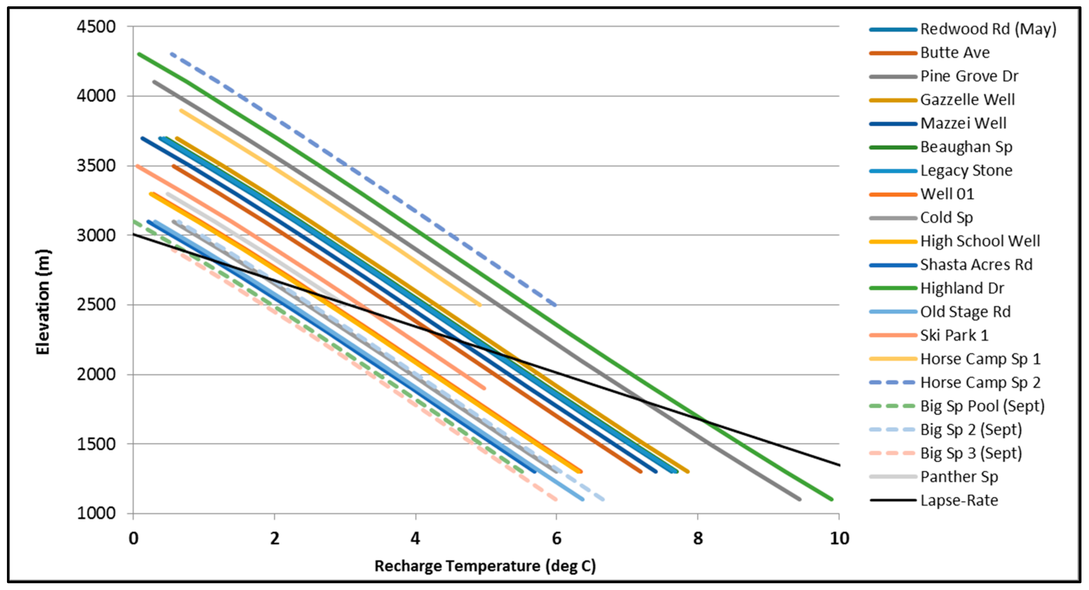
Figure 5.
Land cover for selected spatial area, with well and spring locations (black symbols), 250 m elevation contours and the 14 km radius. The groundwater recharge elevation band indicated by the stable isotope and recharge temperature results is highlighted in (a) by black contours at 2000 m and 2900 m. Maps showing annual precipitation (P; (b)), annual evapotranspiration (ET; (c)) and annual precipitation excess (P−ET; (d)), with a 14-km radius from the summit shown as a black line. Evapotranspiration based on MODIS NDVI (c) is higher at lower elevations but limited in range. Precipitation minus evapotranspiration shows a stark contrast between high elevation barren land and snow cover (above 2500 m) and lower elevation forest cover.

Figure 6.
Mean annual precipitation and temperature for 250 m elevation bins within the 14-km radius in the southwest quadrant of Mt. Shasta (a). The blue bar represents recharge (precipitation minus evapotranspiration), the green bar represents evapotranspiration (ET), the sum being the total precipitation (P). Land cover on south west quadrant of Mt Shasta within a 14 km radius (b) and percentage of total recharge (=P−ET, blue) for each elevation bin. Dark blue box indicates elevation range of recharge derived from stable isotopes and noble gases.

Figure 7.
Discharge temperatures are plotted against sample elevation (a) and δ18O recharge elevation (b). The arrow indicates the increase in temperature between recharge and discharge which is attributed to gravitational energy accumulated along flow paths and geothermal heating. Discharge temperatures corrected for gravitational heating plotted against recharge elevation show the residual geothermal heating (c). Black lines show the expected lapse rate of temperature vs. elevation.

Figure 8.
Topographic cross section of Mt. Shasta within the study area, along with three schematics, example flow paths from recharge areas (as predicted by δ18O results) to sampling locations (dotted line represents a schematic flow path to Horse Camp Spring; solid line to McBride Campground Well; dashed line to Mt Shasta Big Springs). The maximum depth of each flow path is based on the difference between recharge temperatures (predicted by noble gas analyses) and observed discharge temperatures, corrected for gravitational heating. (Vertical exaggeration 4:1).
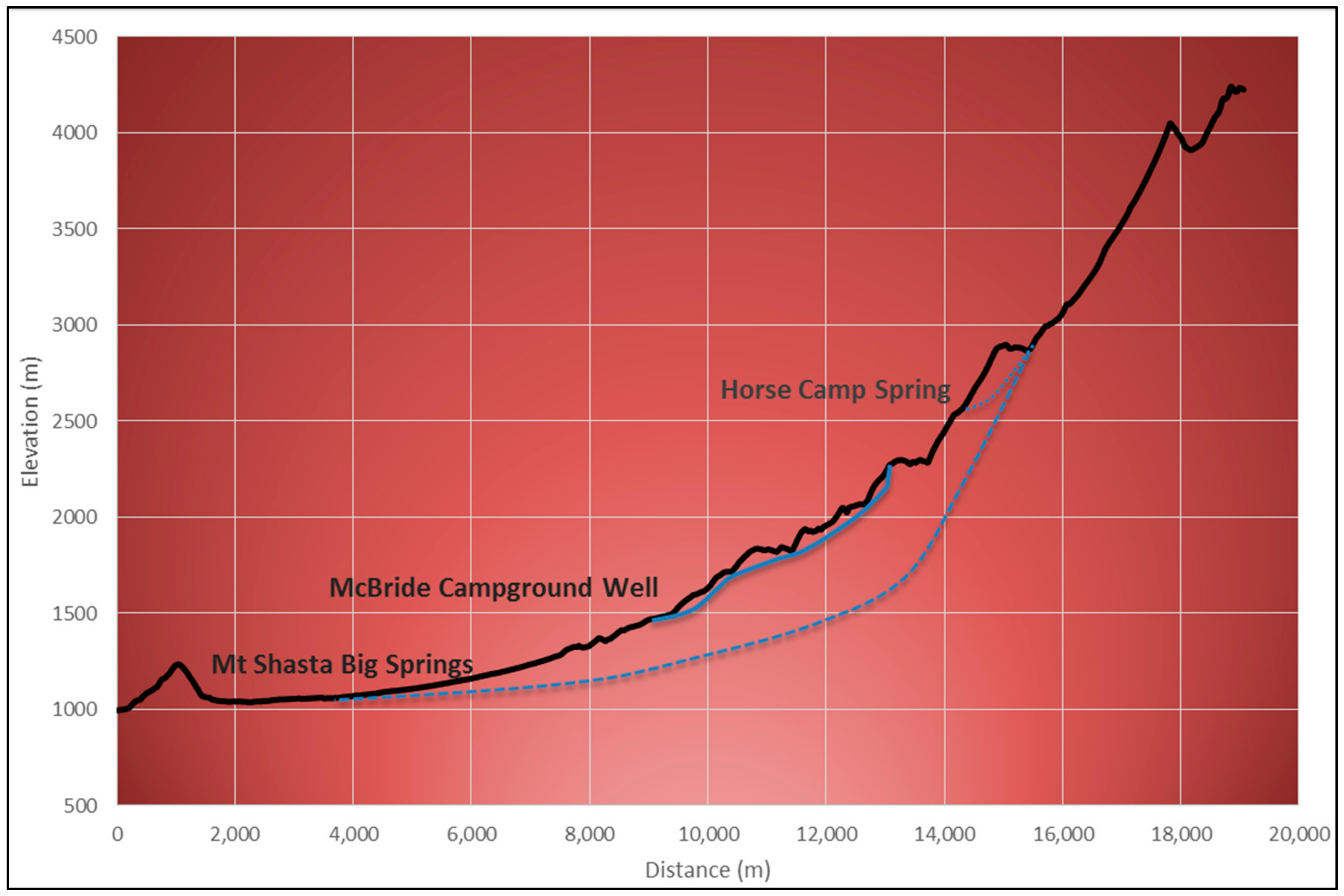
Figure 9.
Tritium activity generally decreases with decreasing sample elevation (Table A5).
Figure 9.
Tritium activity generally decreases with decreasing sample elevation (Table A5).

Figure 10.
Recharge elevation, determined independently from δ18O and noble gas recharge temperature, show good agreement. (Labeled samples are called out in the text.) The box encloses the recharge elevation range used in the spatial analysis.
Figure 10.
Recharge elevation, determined independently from δ18O and noble gas recharge temperature, show good agreement. (Labeled samples are called out in the text.) The box encloses the recharge elevation range used in the spatial analysis.
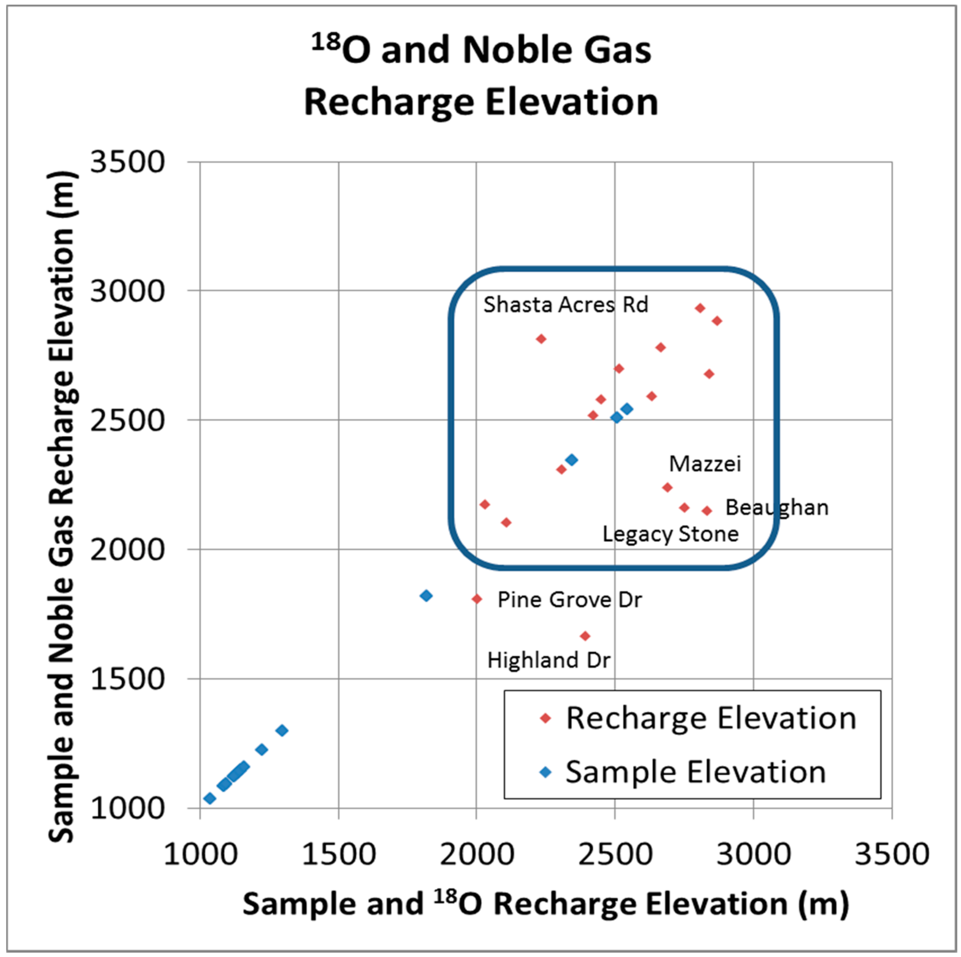
Figure 11.
Evapotranspiration as function of precipitation (a) shows evapotranspiration does not exceed precipitation. A regression between evapotranspiration and mean maximum air temperature (b) shows a significant (R2 = 0.35, p < 0.001) correlation with an increase in evapotranspiration of 45 mm per degree warming for forest land cover.

© 2018 by the authors. Licensee MDPI, Basel, Switzerland. This article is an open access article distributed under the terms and conditions of the Creative Commons Attribution (CC BY) license (http://creativecommons.org/licenses/by/4.0/).
Share and Cite
MDPI and ACS Style
Peters, E.; Visser, A.; Esser, B.K.; Moran, J.E. Tracers Reveal Recharge Elevations, Groundwater Flow Paths and Travel Times on Mount Shasta, California. Water 2018, 10, 97. https://doi.org/10.3390/w10020097
AMA Style
Peters E, Visser A, Esser BK, Moran JE. Tracers Reveal Recharge Elevations, Groundwater Flow Paths and Travel Times on Mount Shasta, California. Water. 2018; 10(2):97. https://doi.org/10.3390/w10020097
Chicago/Turabian StylePeters, Elizabeth, Ate Visser, Bradley K. Esser, and Jean E. Moran. 2018. "Tracers Reveal Recharge Elevations, Groundwater Flow Paths and Travel Times on Mount Shasta, California" Water 10, no. 2: 97. https://doi.org/10.3390/w10020097
Note that from the first issue of 2016, this journal uses article numbers instead of page numbers. See further details here.