Calibration of Spatially Distributed Hydrological Processes and Model Parameters in SWAT Using Remote Sensing Data and an Auto-Calibration Procedure: A Case Study in a Vietnamese River Basin

 ,
,
Abstract
:1. Introduction
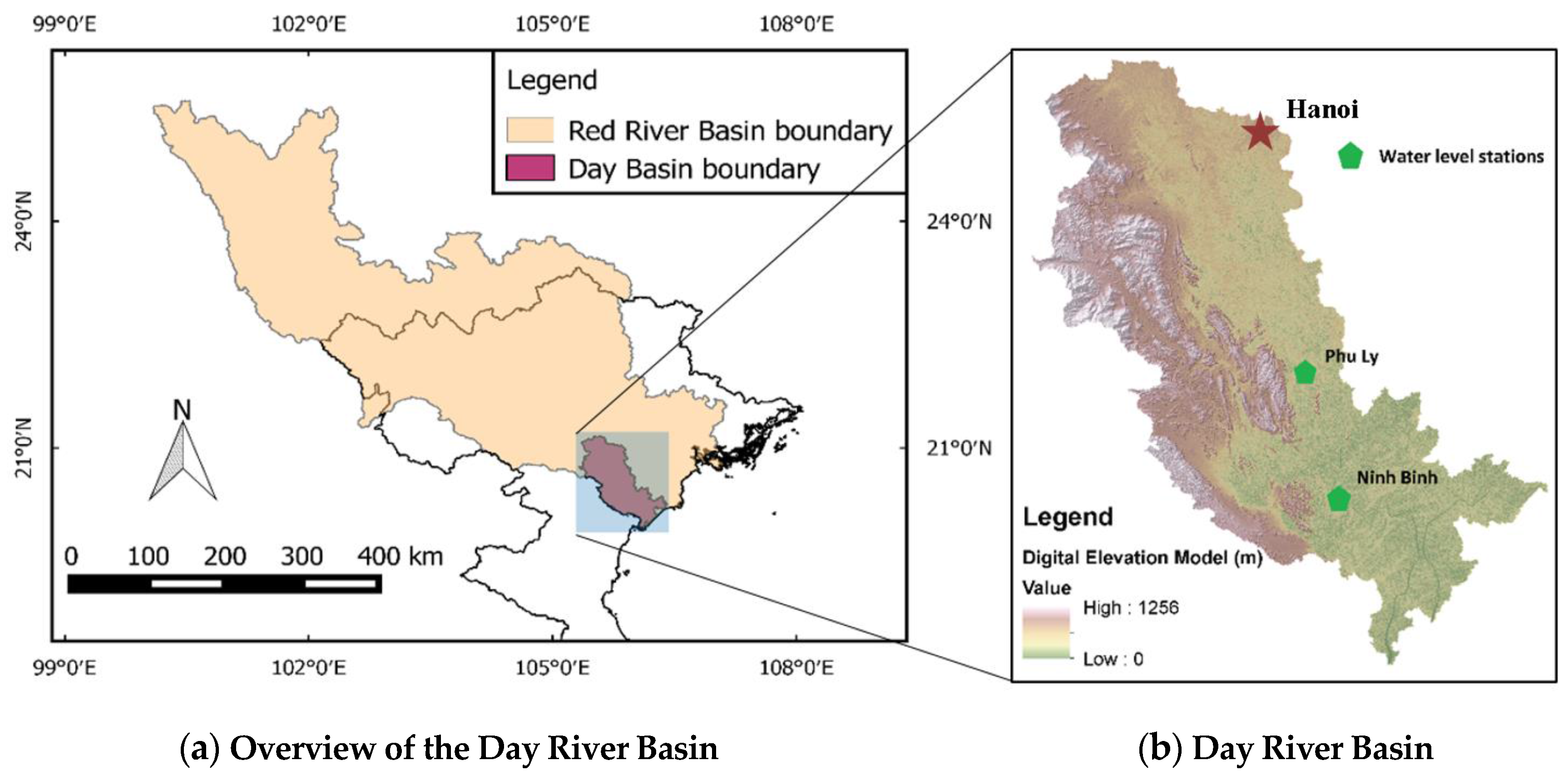
2. Study Area
3. Model and Methodology
3.1. Soil and Water Assessment Tool (SWAT)
3.2. Model Calibration Using SUFI-2
4. Spatial Input Datasets for SWAT
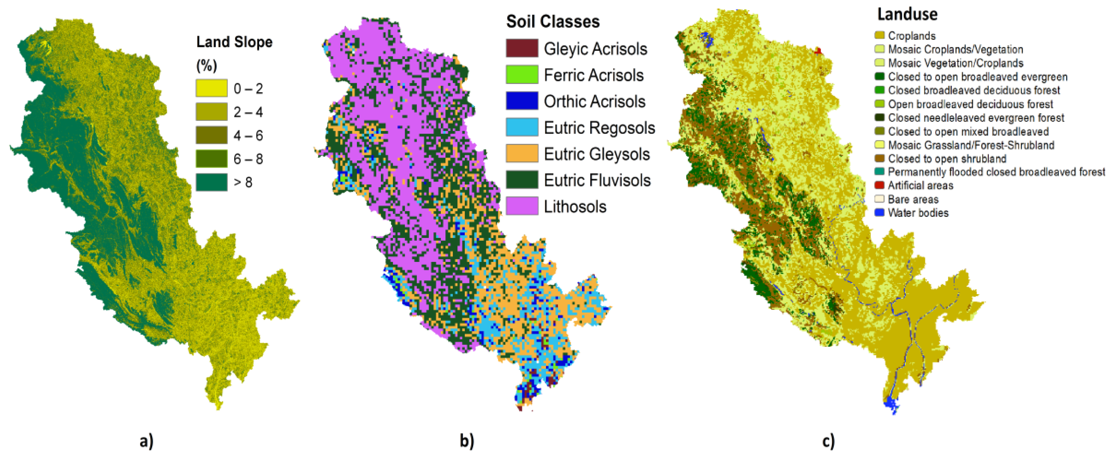
4.1. Physiographical Maps
4.2. Meteorological Data
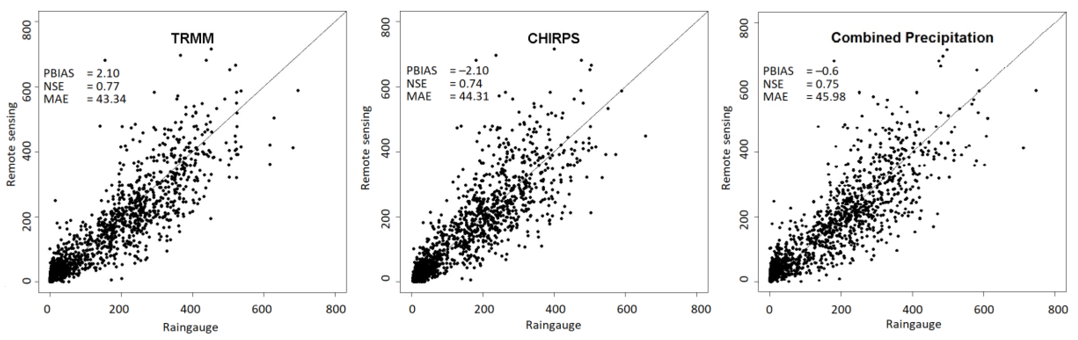
4.2.1. Precipitation
4.2.2. Meteorology
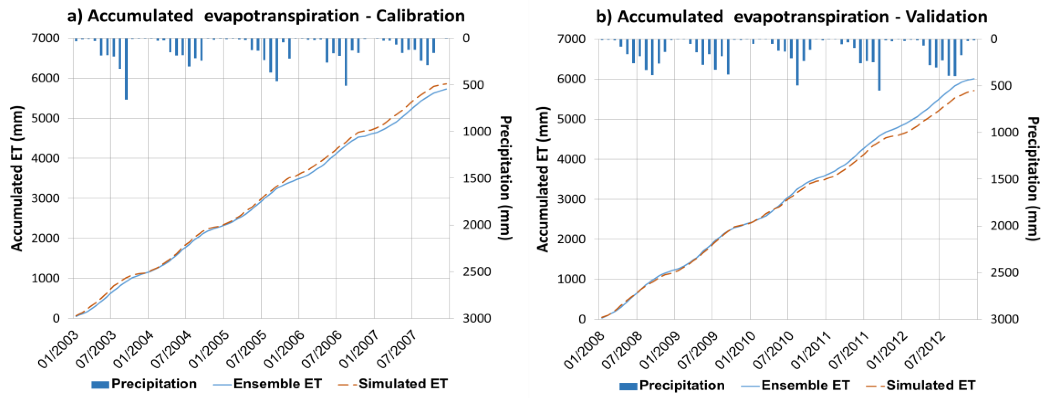
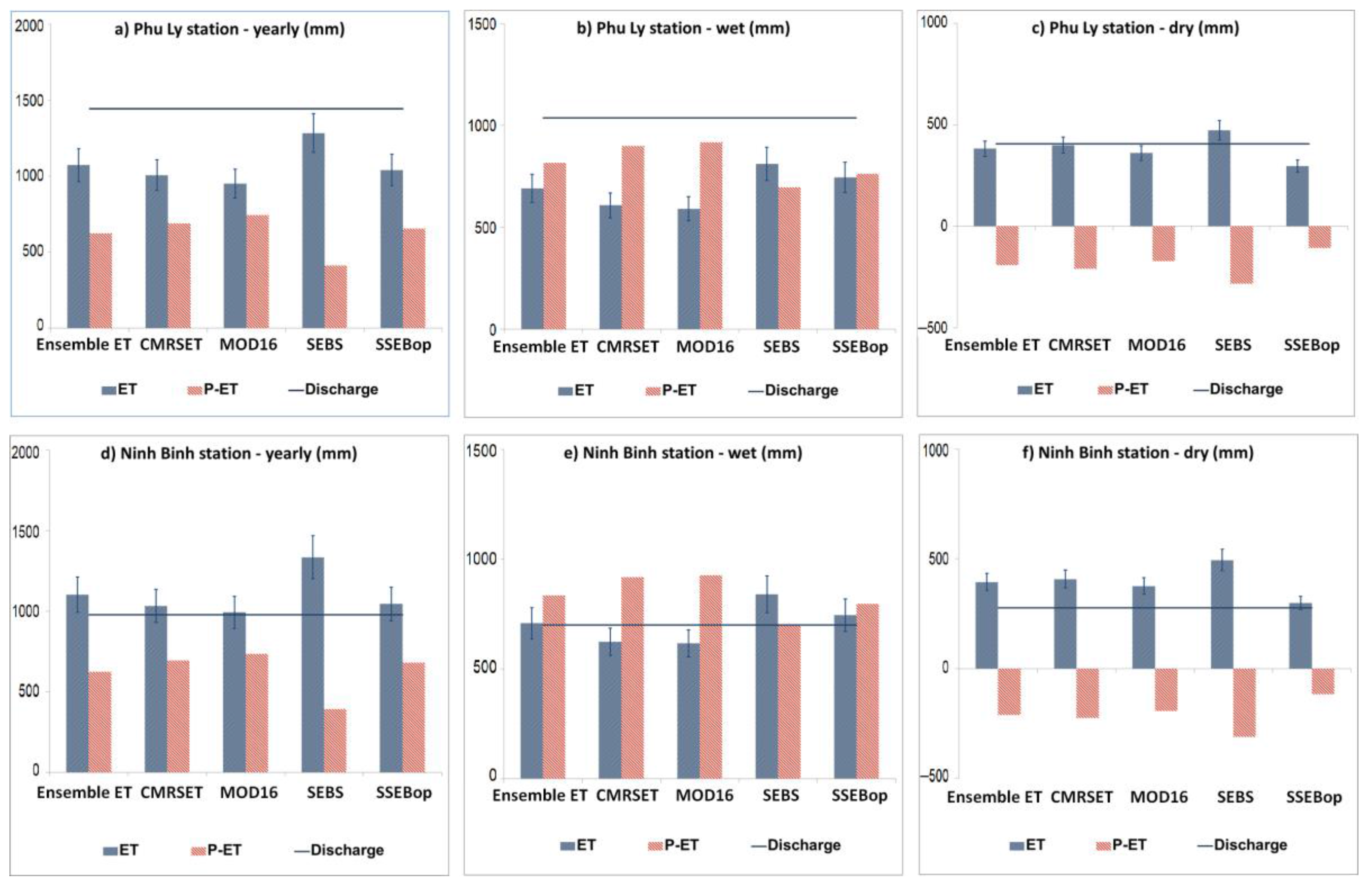
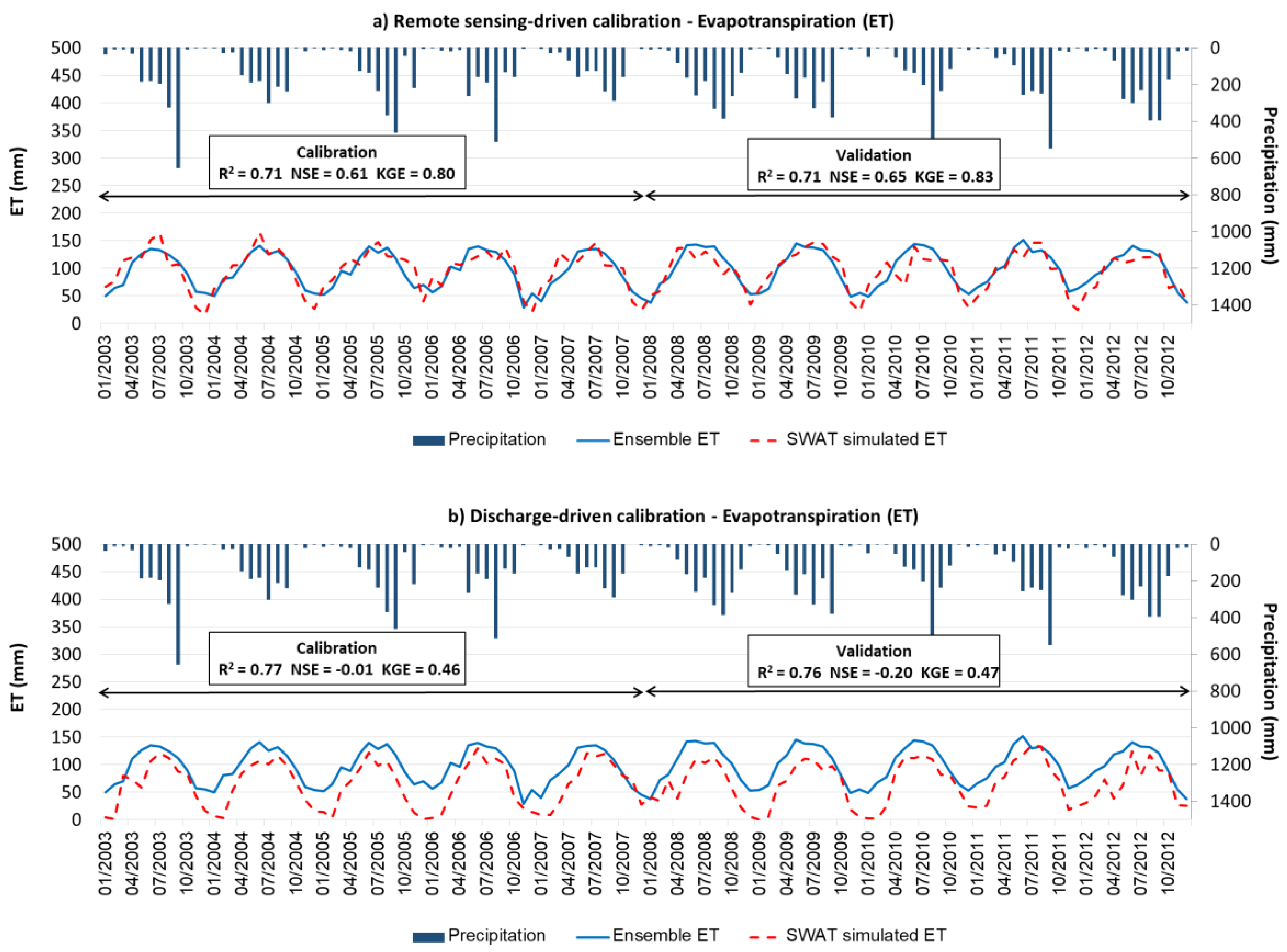
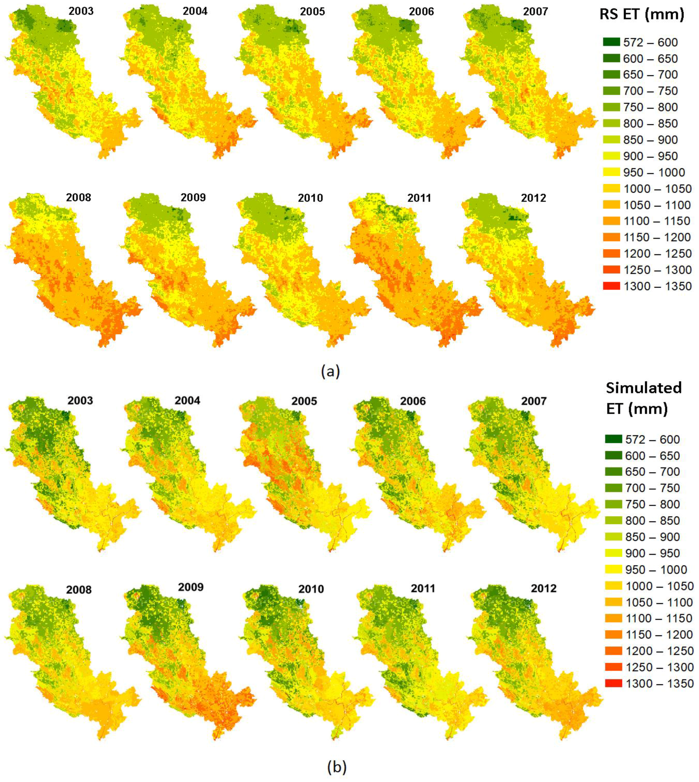
4.2.3. Actual Evapotranspiration
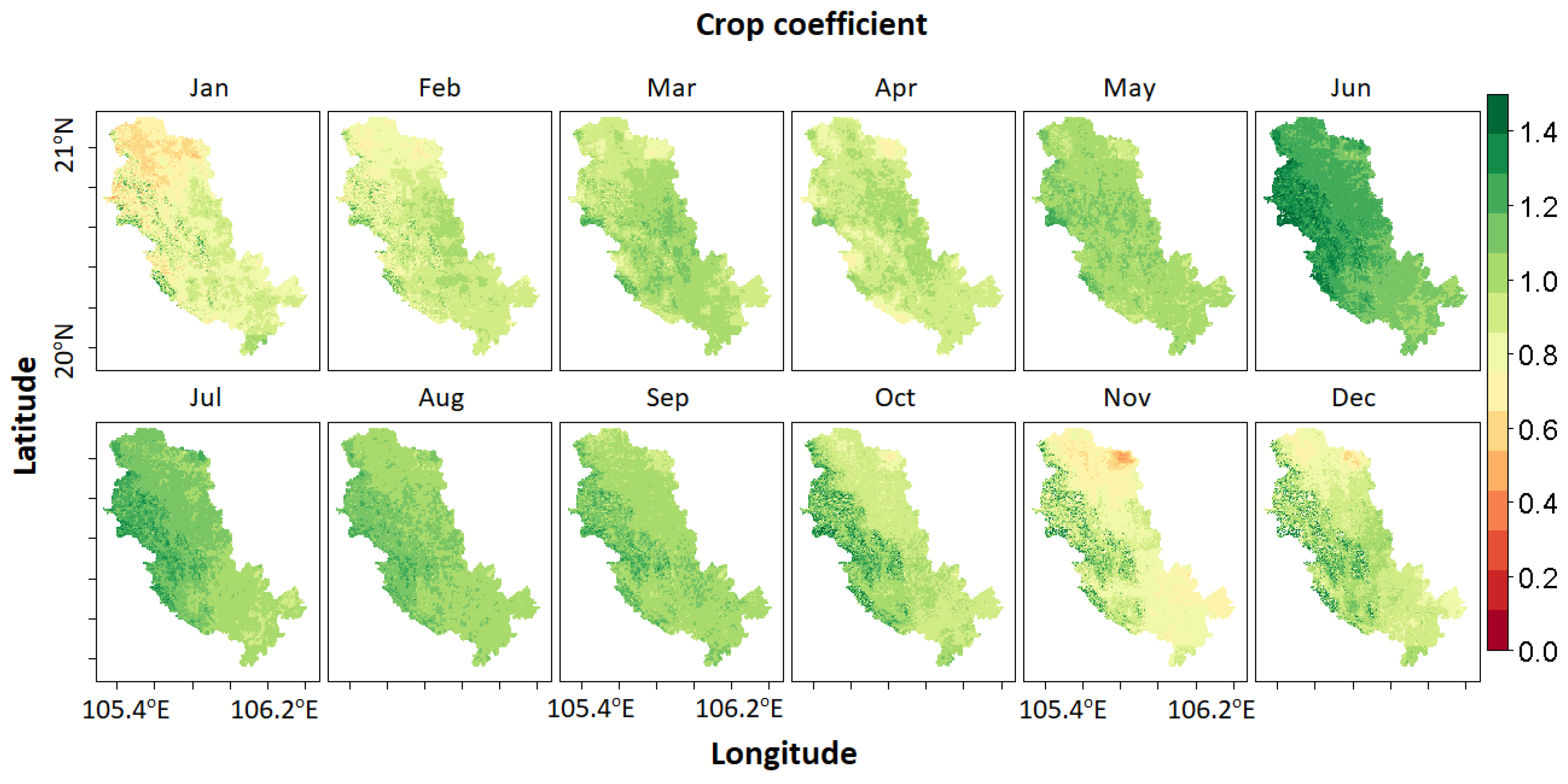
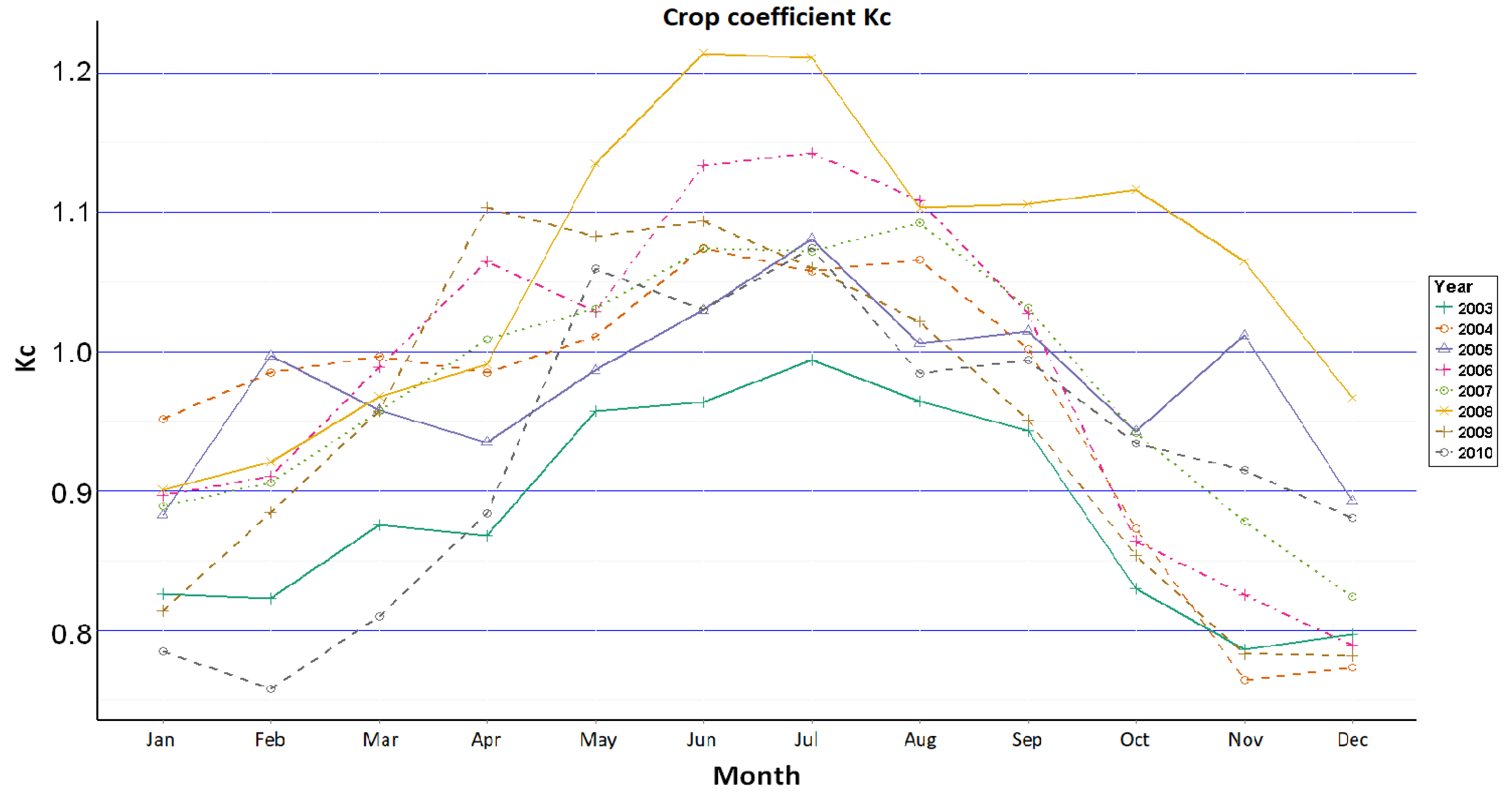
4.2.4. Crop Coefficient
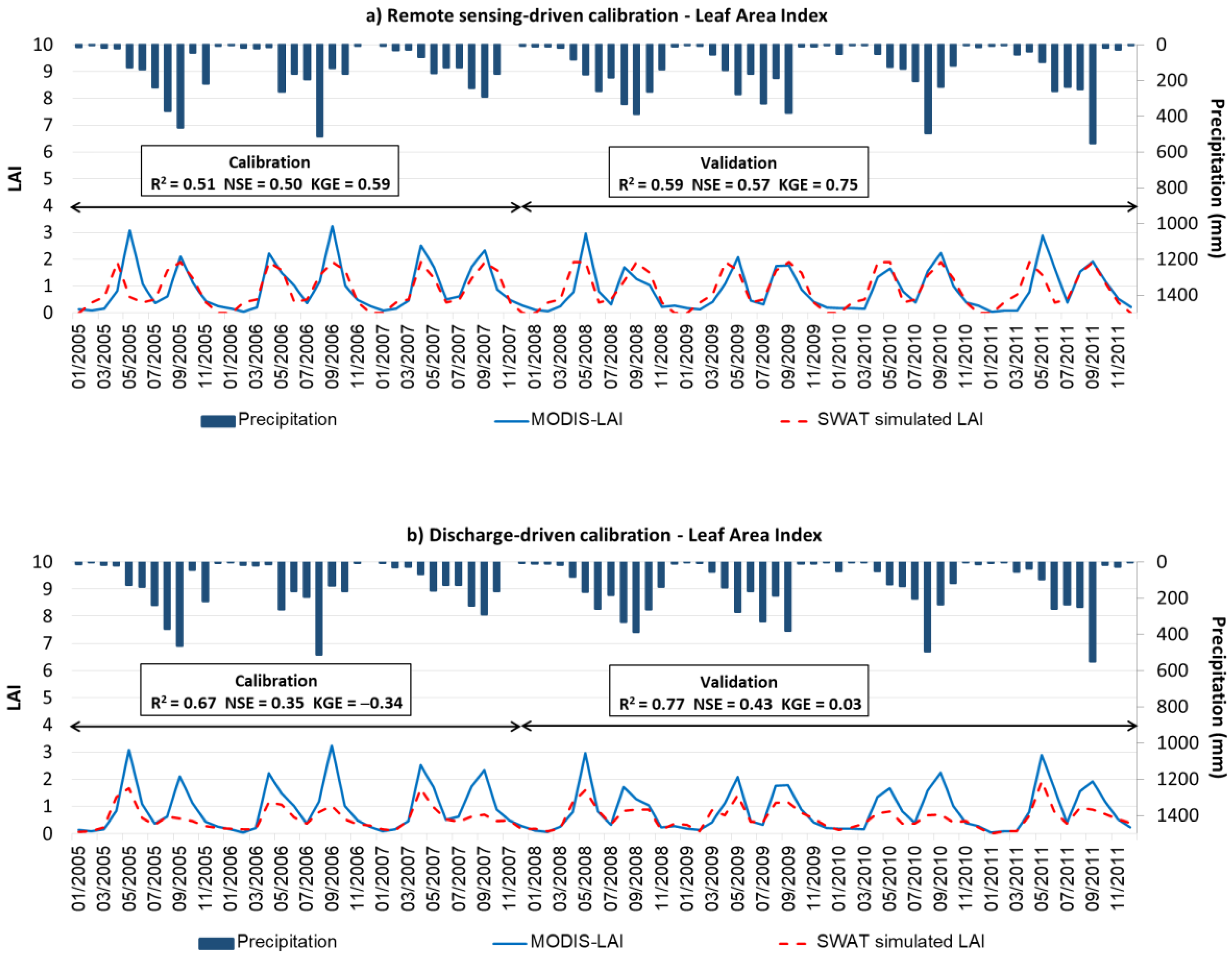
4.3. Leaf Area Index
5. SWAT Parameters to Be Optimized
6. Results and Discussions
7. Conclusions
Acknowledgments
Author Contributions
Conflicts of Interest
References
- Molden, D. Accounting for Water Use and Productivity; SWIM Paper 1; International Irrigation Management Institute: Colombo, Sri Lanka, 1997; p. 26. [Google Scholar]
- Vardon, M.; Lenzen, M.; Peevor, S.; Creaser, M. Water accounting in Australia. Ecol. Econ. 2007, 61, 650–659. [Google Scholar] [CrossRef]
- Karimi, P.; Bastiaanssen, W.G.M.; Molden, D. Water Accounting Plus (WA+)—A water accounting procedure for complex river basins based on satellite measurements. Hydrol. Earth Syst. Sci. 2013, 17, 2459–2472. [Google Scholar] [CrossRef]
- Salvadore, E.; Michailovsky, C.; Coerver, B.; Bastiaanssen, W.G.M. Water Accounting in Selected Asian River, Basins: Pilot Study in Cambodia; Asian Development Bank: Manila, Philippines, 2016; p. 66. [Google Scholar]
- Molden, D.; Frenken, K.; Barker, R.; de Fraiture, C.; Mati, B.; Svendsen, M.; Sadoff, C.; Finlayson, C.M. Trends in water and agricultural development. In Water for Food, Water for Life: A Comprehensive Assessment of Water Management in Agriculture; Molden, D., Ed.; Earthscan: Colombo, Sri Lanka; IWMI: London, UK, 2007; pp. 57–89. [Google Scholar]
- Crossman, N.D.; Burkhard, B.; Nedkov, S.; Willemen, L.; Petz, K.; Palomo, I.; Drakou, E.G.; Martín-Lopez, B.; McPhearson, T.; Boyanova, K.; et al. A blueprint for mapping and modelling ecosystem services. Ecosyst. Serv. 2013, 4, 4–14. [Google Scholar] [CrossRef]
- Bagstad, K.J.; Johnson, G.W.; Voigt, B.; Villa, F. Spatial dynamics of ecosystem service flows: A comprehensive approach to quantifying actual services. Ecosyst. Serv. 2013, 4, 117–125. [Google Scholar] [CrossRef]
- Simons, G.W.H.; Bastiaanssen, W.G.M.; Ngô, L.A.; Hain, C.R.; Anderson, M.C.; Senay, G.B. Integrating Global Satellite-Derived Data Products as a Pre-Analysis for Hydrological Modelling Studies: A Case Study for the Red River Basin. Remote Sens. 2016, 8, 279. [Google Scholar] [CrossRef]
- Vigorstol, K.L.; Aukema, J.E. A comparison of tools for modeling freshwater ecosystem services. J. Environ. Manag. 2011, 92, 2403–2409. [Google Scholar] [CrossRef] [PubMed]
- Arnold, J.G.; Srinivasan, R.; Muttiah, R.S.; Williams, J.R. Large-area hydrologic modeling and assessment: Part I. Model development. J. Am. Water Resour. Assoc. 1998, 34, 73–89. [Google Scholar] [CrossRef]
- Liang, X.; Lettenmaier, D.P.; Wood, E.F.; Burges, S.J. A Simple hydrologically Based Model of Land Surface Water and Energy Fluxes for GSMs. J. Geophys. Res. 1994, 99, 14415–14428. [Google Scholar] [CrossRef]
- Tallis, H.; Polasky, S. Mapping and valuing ecosystem services as an approach for conservation and natural-resource management, The Year in Ecology and Conservation Biology. Ann. N. Y. Acad. Sci. 2009, 1162, 265–283. [Google Scholar] [CrossRef] [PubMed]
- Villa, F.; Athanasiadis, I.N.; Rizzoli, A.E. Modelling with knowledge: A review of emerging semantic approaches to environmental modelling. Environ. Model. Softw. 2009, 24, 577–587. [Google Scholar] [CrossRef]
- Francesconi, W.; Srinivasan, R.; Pérez-Miñana, E.; Willcock, S.P.; Quintero, M. Using the Soil and Water Assessment Tool (SWAT) to model ecosystem services: A systematic review. J. Hydrol. 2016, 535, 625–636. [Google Scholar] [CrossRef]
- Dechmi, F.; Burguete, J.; Skhiri, A. SWAT application in intensive irrigation systems: Model modification, calibration and validation. J. Hydrol. 2012, 470–471, 227–238. [Google Scholar] [CrossRef] [Green Version]
- Gitau, M.W.; Chaubey, I. Regionalization of SWAT Model Parameters for Use in Ungauged Watersheds. Water 2010, 2, 849–871. [Google Scholar] [CrossRef]
- Srinivasan, R.; Zhang, X.; Arnold, J.G. SWAT ungauged: Hydrological budget and crop yield predictions in the upper Mississippi river basin. Trans. ASABE 2010, 53, 1533–1546. [Google Scholar] [CrossRef]
- Schneider, K.; Ketzer, B.; Breuer, L.; Vaché, K.B.; Bernhofer, C.; Frede, H.-G. Evaluation of evapotranspiration methods for model validation in a semi-arid watershed in northern China. Adv. Geosci. 2007, 11, 37–42. [Google Scholar] [CrossRef]
- Van Griensven, A.; Ndomba, P.; Yalew, S.; Kilonzo, F. Critical review of SWAT applications in the upper Nile basin countries. Hydrol. Earth Syst. Sci. 2013, 16, 3371–3381. [Google Scholar] [CrossRef]
- Shrestha, B.; Babel, M.S.; Maskey, S.; van Griensven, A.; Uhlenbrook, S.; Green, A.; Akkharath, I. Impact of climate change on sediment yield in the Mekong River basin: A case study of the Nam Ou basin, Lao PDR. Hydrol. Earth Syst. Sci. 2015, 17, 1–20. [Google Scholar] [CrossRef]
- Raghavan, S.; Tue, V.M.; Shie-Yui, L. Impact of climate change on future stream flow in the Dakbla river basin. J. Hydroinform. 2014, 16, 231–244. [Google Scholar] [CrossRef]
- Abbaspour, K.C.; Rouholahnejad, E.; Vaghefi, S.; Srinivasan, R.; Yang, H.; Kløve, B. A continental-scale hydrology and water quality model for Europe: Calibration and uncertainty of a high-resolution large-scale SWAT model. J. Hydrol. 2015, 524, 733–752. [Google Scholar] [CrossRef]
- Bitew, M.M.; Gebremichael, M. Evaluation of satellite rainfall products through hydrologic simulation in a fully distributed hydrologic model. Water Resour. Res. 2010, 47, W06526. [Google Scholar] [CrossRef]
- Abbaspour, K.C. SWAT-CUP: SWAT Calibration and Uncertainty Programs—A User Manual, Department of Systems Analysis, Integrated Assessment and Modelling (SIAM); Eawag. Swiss Federal Institute of Aquatic Science and Technology: Duebendorf, Switzerland, 2015; p. 100. [Google Scholar]
- Pietroniro, A.; Leconte, R. A review of Canadian remote sensing applications in hydrology, 1995–1999. Hydrol. Process. 2000, 14, 1641–1666. [Google Scholar] [CrossRef]
- Neale, C.M.U.; Cosh, M.H. Remote Sensing and Hydrology; IAHS Red Book Series; Publ. 352; IAHS: Wallingford, UK, 2010; p. 482. [Google Scholar]
- Bastiaanssen, W.G.M.; Harshadeep, N.R. Managing scarce water resources in Asia: The nature of the problem and can remote sensing help? Irrig. Drain. Syst. 2007, 19, 269–284. [Google Scholar] [CrossRef]
- Melesse, A.M.; Weng, Q.; Thenkabail, P.S.; Senay, G.B. Remote Sensing Sensors and Applications in Environmental Resources Mapping and Modelling. Sensors 2016, 7, 3209. [Google Scholar] [CrossRef] [PubMed]
- Serrat-Capdevila, A.; Valdes, J.B.; Stakhiv, E.Z. Water Management Applications for Satellite precipitation products: Synthesis and Recommendations. J. Am. Water Resour. Assoc. 2014, 50, 509–525. [Google Scholar] [CrossRef]
- Dembele, M.; Zwart, J.Z. Evaluation and comparison of satellite-based rainfall products in Burkina Faso, West Africa. Int. J. Remote Sens. 2016, 37, 3995–4014. [Google Scholar] [CrossRef]
- Templeton, R.C.; Vivoni, E.R.; Méndez-Barroso, L.A.; Pierini, N.A.; Anderson, C.A.; Rango, A.; Laliberte, A.S.; Scott, R.L. High-resolution characterization of a semiarid watershed: Implications on evapotranspiration estimates. J. Hydrol. 2014, 509, 306–319. [Google Scholar] [CrossRef]
- Wang-Erlandsson, L.; Bastiaanssen, W.G.M.; Gao, H.; Jägermeyr, J.; Senay, G.B.; van Dijk, A.I.J.M.; Guerschman, J.P.; Keys, P.W.; Gordon, L.J.; Savenije, H.H.G. Global root zone storage capacity from satellite-based evaporation. Hydrol. Earth Syst. Sci. 2016, 20, 1459–1481. [Google Scholar] [CrossRef]
- Li, Z.-L.; Tang, R.; Wan, Z.; Bi, Y.; Zhou, C.; Tang, B.; Yan, G.; Zhang, X. A Review of Current Methodologies for Regional, Evapotranspiration Estimation from Remotely Sensed Data. Sensors 2009, 9, 3801–3853. [Google Scholar] [CrossRef] [PubMed]
- Kalma, J.D.; McVicar, T.R.; McCabe, M.F. Estimating Land Surface Evaporation: A Review of Methods Using Remotely Sensed Surface Temperature Data. Surv. Geophys. 2008, 29, 421–469. [Google Scholar] [CrossRef]
- Senay, G.B.; Leake, S.; Nagler, P.L.; Artan, G.; Dickinson, J.; Cordova, J.T.; Glenn, E.P. Estimating Basin Scale Evapotranspiration (ET) by Water Balance and Remote Sensing Methods. Hydrol. Process. 2011, 25, 4037–4049. [Google Scholar] [CrossRef]
- Karimi, P.; Bastiaanssen, W.G.M. Spatial evapotranspiration, rainfall and land use data in water accounting—Part 1: Review of the accuracy of the remote sensing data. Hydrol. Earth Syst. Sci. 2015, 19, 507–532. [Google Scholar] [CrossRef]
- Carlson, T.N.; Ripley, D.A. On the relation between NDVI, fractional vegetation cover, and leaf area index. Remote Sens. Environ. 1997, 62, 241–252. [Google Scholar] [CrossRef]
- Droogers, P.; Bastiaanssen, W.G.M. Irrigation Performance using Hydrological and Remote Sensing Modeling. J. Irrig. Drain Eng. 2002, 128, 11–18. [Google Scholar] [CrossRef]
- Schuurmans, J.M.; Troch, P.A.; Veldhuizen, A.A.; Bastiaanssen, W.G.M.; Bierkens, M.F.P. Assimilation of remotely sensed latent heat flux in a distributed hydrological model. Adv. Water Resour. 2003, 26, 151–159. [Google Scholar] [CrossRef]
- Vazifedoust, M.; van Dam, J.C.; Feddes, R.A.; Feizi, M. Increasing water productivity of irrigated crops under limited water supply at field scale. Agric. Water Manag. 2008, 95, 89–102. [Google Scholar] [CrossRef]
- Jhorar, R.K.; Smit, A.A.M.F.R.; Bastiaanssen, W.G.M.; Roest, C.W.J. Calibration of a distributed irrigation water management model using remotely sensed evapotranspiration rates and groundwater heads. Irrig. Drain. 2011, 60, 57–69. [Google Scholar] [CrossRef]
- Githui, F.; Selle, B.; Thayalakumaran, T. Recharge estimation using remotely sensed evapotranspiration in an irrigated catchment in southeast Australia. Hydrol. Process. 2011, 26, 1379–1389. [Google Scholar] [CrossRef]
- Immerzeel, W.W.; Droogers, P. Calibration of a distributed hydrological model based on satellite evapotranspiration. J. Hydrol. 2008, 349, 411–424. [Google Scholar] [CrossRef]
- Immerzeel, W.W.; Gaur, A.; Zwart, S.J. Integrating remote sensing and a process-based hydrological model to evaluate water use and productivity in a south Indian catchment. Agric. Water Manag. 2007, 95, 11–24. [Google Scholar] [CrossRef]
- Cheema, M.J.M.; Immerzeel, W.W.; Bastiaanssen, W.G.M. Spatial Quantification of Groundwater Abstraction in the Irrigated Indus Basin. Ground Water 2014, 52, 25–36. [Google Scholar] [CrossRef] [PubMed]
- Sun, C.; Jiang, D.; Wang, J.; Zhu, Y. Validating remote sensing derived evapotranspiration with the soil and water assessment tool (SWAT) model: A case study in Zhelin Basin, China. Afr. J. Agric. Res. 2013, 8, 2090–2098. [Google Scholar] [CrossRef]
- Sousa, A.M.L.; Vitorino, M.I.; Castro, N.M.R.; Botelho, M.N.; Souza, P.J.O.P. Evapotranspiration from Remote Sensing to Improve the SWAT Model in Eastern Amazonia. Floresta Ambient. 2015, 22, 456–464. [Google Scholar] [CrossRef]
- Bréda, N.J.J. Ground-based measurements of leaf area index: A review of methods, instruments and current controversies. J. Exp. Bot. 2003, 54, 2403–2417. [Google Scholar] [CrossRef] [PubMed]
- Van Griensven, A.; Maskey, S.; Stefanova, A. The use of satellite images for evaluating a SWAT model: Application on the Vit Basin, Bulgaria. In International Environmental Modelling and Software Society (iEMSs) International Congress on Environmental Modelling and Software: Managing Resources of a Limited Planet: Pathways and Visions under Uncertainty, Sixth Biennial Meeting; Seppelt, R., Voinov, A.A., Lange, S., Bankamp, D., Eds.; the International Environmental Modelling and Software Society (iEMSs): Leipzig, Germany, 2012; pp. 3030–3037. ISBN 978-88-9035-742-8. [Google Scholar]
- Luu, T.N.M.; Garnier, J.; Billen, G.; Orange, D.; Néméry, J.; Le, T.P.Q.; Tran, H.T.; Le, L.A. Hydrological regime and water budget of the Red River Delta (Northern Vietnam). J. Asian Earth Sci. 2010, 37, 219–228. [Google Scholar] [CrossRef]
- Le, T.P.Q.; Billen, G.; Garnier, J.; Théry, S.; Fézard, C.; Chau, V.M. Nutrient (N, P) budgets for the Red River basin (Vietnam and China). Glob. Biogeochem. Cycles 2005, 19, GB2022. [Google Scholar] [CrossRef]
- Giuliani, M.; Anghileri, D.; Castelletti, A.; Vu, P.N.; Soncini-Sessa, R. Large storage operations under climate change: Expanding uncertainties and evolving tradeoffs. Environ. Res. Lett. 2016, 11, 035009. [Google Scholar] [CrossRef]
- Neitsch, S.L.; Arnold, J.G.; Kiniry, J.R.; Williams, J.R. Soil and Water Assessment Tool Theoretical Documentation Version 2009; Texas Water Resources Institute: College Station, TX, USA, 2011. [Google Scholar]
- Arnold, J.G.; Moriasi, D.N.; Gassman, P.W.; Abbaspour, K.C.; White, M.J.; Srinivasan, R.; Santhi, C.; Harmel, R.D.; Van Griensven, A.; Van Liew, M.W.; et al. SWAT: Model use, calibration, and validation. Trans. ASABE 2012, 55, 1491–1508. [Google Scholar] [CrossRef]
- Cibin, R.; Sudheer, K.P.; Chaubey, I. Sensitivity and identifiability of stream flow generation parameters of the SWAT model. Hydrol. Process. 2010, 24, 1133–1148. [Google Scholar] [CrossRef]
- Hargreaves, G.; Hargreaves, G.; Riley, J. Agricultural Benefits for Senegal River Basin. J. Irrig. Drain Eng 1985, 111, 113–124. [Google Scholar] [CrossRef]
- Priestley, C.H.B.; Taylor, R.J. On the assessment of surface heat flux and evaporation using large scale parameters. Mon. Weather Rev. 1972, 100, 81–92. [Google Scholar] [CrossRef]
- Abbaspour, K.C.; van Genuchten, M.T.; Schulin, R.; Schläppi, E. A sequential uncertainty domain inverse procedure for estimating subsurface flow and transport parameters. Water Resour. Res. 1997, 33, 1879–1892. [Google Scholar] [CrossRef]
- Strauch, M.; Volk, M. SWAT plant growth modification for improved modeling of perennial vegetation in the tropics. Ecol. Model. 2013, 269, 98–112. [Google Scholar] [CrossRef]
- Arino, O.; Bicheron, P.; Achard, F.; Latham, J.; Witt, R.; Weber, J.-L. GLOBCOVER the most detailed portrait of Earth. ESA Bull. 2008, 136, 24–31. [Google Scholar]
- Hengl, T.; de Jesus, J.M.; MacMillan, R.A.; Batjes, N.H.; Heuvelink, G.B.M.; Ribeiro, E.; Samuel-Rosa, A.; Kempen, B.; Leenaars, J.G.B.; Walsh, M.G.; et al. SoilGrids1km—Global Soil Information Based on Automated Mapping. PLoS ONE 2014, 9, e105992. [Google Scholar] [CrossRef] [PubMed]
- Food and Agricultural Organization (FAO). The Digital Soil Map of the World and Derived Soil Properties [CD-ROM]; Version 3.5; Food and Agricultural Organization: Rome, Italy, 1995. [Google Scholar]
- Meng, J.; Li, L.; Hao, Z.; Wang, J.; Shao, Q. Suitability of TRMM satellite rainfall in driving a distributed hydrological model in the source region of yellow river. J Hydrol. 2014, 509, 320–332. [Google Scholar] [CrossRef]
- Li, Z.; Yang, D.; Gao, B.; Jiao, Y.; Hong, Y.; Xu, T. Multi-scale Hydrologic Applications of the Latest Satellite Precipitation Products in the Yangtze River Basin using a Distributed Hydrologic Model. J. Hydr. 2015, 16, 407–426. [Google Scholar] [CrossRef]
- Pena-Arancibia, J.L.; van Dijk, A.I.J.M.; Renzullo, L.J.; Mulligan, M. Evaluation of Precipitation Estimation Accuracy in Reanalyses, Satellite Products, and an Ensemble Method for Regions in Australia and South and East Asia. J. Hydrometeorol. 2013, 14, 1323–1333. [Google Scholar] [CrossRef] [Green Version]
- Funk, C.C.; Peterson, P.J.; Landsfeld, M.F.; Pedreros, D.H.; Verdin, J.P.; Rowland, J.D.; Romero, B.E.; Husak, G.J.; Michaelsen, J.C.; Verdin, A.P. A Quasi-Global Precipitation Time Series for Drought Monitoring; Data Series 832; U.S. Geological Survey: Reston, VA, USA, 2014; p. 4.
- Toté, C.; Patricio, D.; Boogaard, H.L.; van der Wijngaart, R.; Tarnavsky, E.; Funk, C. Evaluation of Satellite Rainfall Estimates for Drought and Flood Monitoring in Mozambique. Remote Sens. 2015, 7, 1758–1776. [Google Scholar] [CrossRef]
- Rodell, M.; Houser, P.R.; Jambor, U.; Gottschalck, J.; Mitchell, K.; Meng, C.-J.; Arsenault, K.; Cosgrove, B.; Radakovich, J.; Bosilovich, M.; et al. The Global Land Data Assimilation System. Bull. Am. Met. Soc. 2004, 85, 381–394. [Google Scholar] [CrossRef]
- Mu, Q.Z.; Heinsch, F.A.; Zhao, M.; Running, S.W. Development of a global evapotranspiration algorithm based on MODIS and global meteorology data. Remote Sens. Environ. 2007, 111, 519–536. [Google Scholar] [CrossRef]
- Hu, G.; Jia, L.; Menenti, M. Comparison of MOD16 and LSA-SAF MSG evapotranspiration products over Europe for 2011. Remote Sens. Environ. 2015, 156, 510–526. [Google Scholar] [CrossRef]
- Ramoelo, A.; Majozi, N.; Mathieu, R.; Jovanovic, N.; Nickless, A.; Dzikiti, S. Validation of Global Evapotranspiration Product (MOD16) using Flux Tower Data in the African Savanna, South Africa. Remote Sens. 2014, 6, 7406–7423. [Google Scholar] [CrossRef]
- Trambauer, P.; Dutra, E.; Maskey, S.; Werner, M.; Pappenberger, F.; van Beek, L.P.H.; Uhlenbrook, S. Comparison of different evaporation estimates over the African continent. Hydrol. Earth Syst. Sci. 2014, 18, 193–212. [Google Scholar] [CrossRef] [Green Version]
- Knipper, K.R.; Kinoshita, A.M.; Hogue, T.S. Evaluation of a moderate resolution imaging spectroradiometer triangle-based algorithm for evapotranspiration estimates in subalpine regions. J. Appl. Remote Sens. 2016, 10, 016002. [Google Scholar] [CrossRef]
- Su, Z. The Surface Energy Balance System (SEBS) for estimation of turbulent heat fluxes. Hydrol. Earth Syst. Sci. 2002, 6, 85–100. [Google Scholar] [CrossRef]
- Chen, X.; Su, Z.; Ma, Y.; Yang, K.; Wen, J.; Zhang, Y. An Improvement of Roughness Height Parameterization of the Surface Energy Balance System (SEBS) over the Tibetan Plateau. J. Appl. Meteorol. Climatol. 2013, 52, 607–622. [Google Scholar] [CrossRef]
- Guerschman, J.P.; van Dijk, A.I.J.M.; Mattersdorf, G.; Beringer, J.; Hutley, L.B.; Leuning, R.; Pipunic, R.C.; Sherman, B.S. Scaling of potential evapotranspiration with MODIS data reproduces flux observations and catchment water balance observations across Australia. J. Hydrol. 2009, 369, 107–119. [Google Scholar] [CrossRef]
- Priestley, C.H.B.; Taylor, R.J. On the assessment of surface heat flux and evaporation using large scale parameters. Mon. Weather Rev. 1972, 100, 81–92. [Google Scholar] [CrossRef]
- Senay, G.B.; Budde, M.; Verdin, J.P.; Melesse, A.M. A coupled remote sensing and simplified surface energy balance approach to estimate actual evapotranspiration from irrigated fields. Sensors 2007, 7, 979–1000. [Google Scholar] [CrossRef]
- Senay, G.B.; Bohms, S.; Singh, R.K.; Gowda, P.H.; Velpuri, N.M.; Alemu, H.; Verdin, J. Operational evapotranspiration modeling using remote sensing and weather datasets: A new parameterization for the SSEB ET approach. J. Am. Water Resour. Assoc. 2013, 49, 577–591. [Google Scholar] [CrossRef]
- Kim, H.W.; Hwang, K.; Mu, Q.; Lee, O.S.; Choi, M. Validation of MODIS 16 global terrestrial evapotranspiration products in various climates and land cover types in Asia. KSCE J. Civil. Eng. 2012, 16, 229–238. [Google Scholar] [CrossRef]
- Westerhoff, R.S. Using Uncertainty of Penman and Penman–Monteith Methods in Combined Satellite and Ground-Based Evapotranspiration Estimates. Remote Sens. Environ. 2015, 169, 102–112. [Google Scholar] [CrossRef]
- Bastiaanssen, W.G.M.; Allen, R.G.; Pelgrum, H.; de C. Texeira, A.H.; Soppe, R.W.O.; Thoreson, B.P. Thermal-infrared technology for local and regional scale irrigation analyses in horticultural systems. Acta Hortic. 2008, 792, 33–46. [Google Scholar] [CrossRef]
- Ferguson, C.R.; Sheffield, J.; Wood, E.F.; Gao, H. Quantifying uncertainty in a remote sensing-based estimate of evapotranspiration over continental USA. Int. J. Remote Sens. 2010, 31, 3821–3865. [Google Scholar] [CrossRef]
- Bastiaanssen, W.G.M.; Hoekman, D.H.; Roebeling, R.A. A methodology for the assessment of surface resistance and soil water storage variability at mesoscale based on remote sensing measurements. In IAHS Special Publications; No. 2; IAHS: Wallingford, UK, 1993; p. 63. [Google Scholar]
- Allen, R.G.; Pereira, L.S.; Raes, D.; Smith, M. Crop Evapotranspiration: Guidelines for Computing Crop Water Requirements; FAO Irrigation and Drainage Paper No. 56; FAO: Rome, Italy, 1998; p. 300. [Google Scholar]
- Mohan, S.; Arumugam, N. Irrigation crop coefficients for lowland rice. Irrig. Drain. Syst. 1994, 8, 159–176. [Google Scholar] [CrossRef]
- Vu, H.S.; Watanabe, H.; Takagi, K. Application of FAO-56 for evaluating evapotranspiration in simulation of pollutant runoff from paddy rice field in Japan. Agric. Water Manag. 2005, 76, 195–210. [Google Scholar] [CrossRef]
- Tyagi, N.K.; Sharma, D.K.; Luthra, S.K. Determination of evapotranspiration and crop coefficients of rice and sunflower with lysimeter. Agric. Water Manag. 2000, 45, 41–54. [Google Scholar] [CrossRef]
- Abdullahi, A.S.; Soom, M.A.M.; Ahmad, D.; Shariff, A.R.M. Characterization of rice (Oryza Sativa) evapotranspiration using micro paddy lysimeter and class “A” pan in tropical environments, Australian. J. Crop Sci. 2013, 7, 650–680. [Google Scholar]
- Stisen, S.; Jensen, K.H.; Sandholt, I.; Grimes, D.I. A remote sensing driven distributed hydrological model of the Senegal River basin: A remote sensing-driven model. J. Hydrol. 2008, 354, 131–148. [Google Scholar] [CrossRef]


| Unsaturated Zone | |||||||||||
| Year | Input | Output | ∆u | ||||||||
| P | IRR | Revap | Qrunoff | Qlat | ET | PERC | ∆ER | ||||
| Average | 1709.5 | 309.2 | 19.4 | 586.9 | 14.0 | 957.9 | 441.5 | 49.5 | −11.7 | ||
| 2007 | 1496.1 | 302.0 | 3.6 | 447.2 | 11.1 | 985.0 | 347.9 | −27.1 | 37.7 | ||
| 2008 | 2121.1 | 375.7 | 0.7 | 789.1 | 15.8 | 1009.5 | 606.2 | 80.1 | −3.2 | ||
| Saturated Zone | |||||||||||
| Year | Input | Output | ∆u | ||||||||
| PERC | Revap | GW_RCH | SA_ST | ||||||||
| Average | 441.5 | 19.4 | 436.1 | −23.6 | 9.6 | ||||||
| 2007 | 347.9 | 3.6 | 358.0 | −7.8 | −5.9 | ||||||
| 2008 | 606.2 | 0.7 | 487.7 | 0.0 | 117.9 | ||||||
| Parameter | Unit ** | Default Range * | Final Value |
|---|---|---|---|
| ESCO | - | 0–1 | 0–0.22 |
| EPCO | - | 0–1 | 0.88–1.00 |
| REVAPMN | mm | 0–500 | 248–395 |
| SOL_K | mm/hr | 0–2000 | 0.44–1262 |
| SOL_AWC | mm water/mm soil | 0–1 | 0.50–1 |
| SOL_BD | mg/m3 or g/cm3 | 1.1–1.9 | 1.2–1.62 |
| CN2 | - | 35–98 | 72.9–98 |
| ALPHA_BF | - | 0–1 | 0.42–0.75 |
| BLAI | m2/m2 | 0.5–10 | 0.89–10 |
| ALAI_MIN | m2/m2 | 0–0.99 | 0–0.98 |
| DLAI | - | 0.15–1 | 0.30–0.95 |
| LAIMX1 | - | 0–1 | 0–0.75 |
| LAIMX2 | - | 0–1 | 0–0.99 |
| FRGRW1 | - | 0–1 | 0–0.76 |
| FRGRW2 | - | 0–1 | 0–0.74 |
© 2018 by the authors. Licensee MDPI, Basel, Switzerland. This article is an open access article distributed under the terms and conditions of the Creative Commons Attribution (CC BY) license (http://creativecommons.org/licenses/by/4.0/).
Share and Cite
Ha, L.T.; Bastiaanssen, W.G.M.; Van Griensven, A.; Van Dijk, A.I.J.M.; Senay, G.B. Calibration of Spatially Distributed Hydrological Processes and Model Parameters in SWAT Using Remote Sensing Data and an Auto-Calibration Procedure: A Case Study in a Vietnamese River Basin. Water 2018, 10, 212. https://doi.org/10.3390/w10020212
Ha LT, Bastiaanssen WGM, Van Griensven A, Van Dijk AIJM, Senay GB. Calibration of Spatially Distributed Hydrological Processes and Model Parameters in SWAT Using Remote Sensing Data and an Auto-Calibration Procedure: A Case Study in a Vietnamese River Basin. Water. 2018; 10(2):212. https://doi.org/10.3390/w10020212
Chicago/Turabian StyleHa, Lan Thanh, Wim G. M. Bastiaanssen, Ann Van Griensven, Albert I. J. M. Van Dijk, and Gabriel B. Senay. 2018. "Calibration of Spatially Distributed Hydrological Processes and Model Parameters in SWAT Using Remote Sensing Data and an Auto-Calibration Procedure: A Case Study in a Vietnamese River Basin" Water 10, no. 2: 212. https://doi.org/10.3390/w10020212