The Significance of the Spatial Variability of Rainfall on the Numerical Simulation of Urban Floods


1
Instituto de Ingeniería, Universidad Nacional Autónoma de México, Circuito Escolar, Ciudad Universitaria, Coyoacán 04510, Ciudad de México, Mexico
2
Programa de Maestria y Doctorado en Ingeniería, Universidad Nacional Autónoma de México, Circuito Exterior, Ciudad Universitaria, Coyoacán 04510, Ciudad de México, Mexico
3
Department of Civil Engineering, University of Bristol, University Walk, Clifton BS8 1TR, Bristol, UK
*
Author to whom correspondence should be addressed.
Water 2018, 10(2), 207; https://doi.org/10.3390/w10020207
Submission received: 30 August 2017
/
Revised: 12 December 2017
/
Accepted: 12 December 2017
/
Published: 15 February 2018
Abstract
:The growth of urban population, combined with an increase of extreme events due to climate change call for a better understanding and representation of urban floods. The uncertainty in rainfall distribution is one of the most important factors that affects the watershed response to a given precipitation event. However, most of the investigations on this topic have considered theoretical scenarios, with little reference to case studies in the real world. This paper incorporates the use of spatially-variable precipitation data from a long-range radar in the simulation of the severe floods that impacted the city of Hull, U.K., in June 2007. This radar-based rainfall field is merged with rain gauge data using a Kriging with External Drift interpolation technique. The utility of this spatially-variable information is investigated through the comparison of computed flooded areas (uniform and radar) against those registered by public authorities. Both results show similar skills at reproducing the real event, but differences in the total precipitated volumes, water depths and flooded areas are illustrated. It is envisaged that in urban areas and with the advent of higher resolution radars, these differences will be more important and call for further investigation.
1. Introduction
With the advent of computational methods and computer processing power, the ability to tackle urban floods at the catchment level is clearly emerging, making it possible to apply an integrated approach to modelling rainfall-runoff processes along with surface flows [1,2]. Moreover, the availability of new data sources with higher quality and spatio-temporal resolution (e.g., rainfall data estimated by radars and terrain data derived from Lidar Detection and Ranging (LiDAR)) enables a more detailed description of hydrological processes that occur in the real world, paving the road towards a better numerical discretisation of the processes involved in urban floods.
On the other hand, the documented growth in the number of floods and urban population due to climate change [3] clearly indicates the importance of an improved understanding of how flood waters interact with the urban environment both in space and time. Indeed, the development of a reliable approach to adequately describe urban flood processes has been recognised as a challenging task [4].
Recent advances in urban flood modelling recognise the importance of 2D modelling algorithms to adequately reproduce urban floods [5]. However, it should be borne in mind that model performance also depends on the quality of data used to construct a numerical representation of the catchment. This information includes soil characteristics, land use, topography and forcing conditions, all of which play an important role in the generation of an urban flood [6,7]. In reality, these data vary in space and time, and their representation at an adequate spatio-temporal resolution is necessary for an accurate performance of the numerical tool. However, datasets are rarely homogeneous in space and time, which leaves the door open to the exploration of an adequate level of complexity and detail for this purpose.
Among the main factors identified to adequately reproduce urban floods, the uncertainty of rainfall distribution in time and space is one of the main sources of error [8]. It is well known that a good knowledge of precipitation at appropriate spatial and temporal scales enhances modelling of rainfall-runoff processes in urban catchments [8,9,10,11,12,13]. Accurate estimations of precipitation in urban areas require a dense rain gauge network combined with an effective analysis method. However, rain gauge networks are generally too sparse spatially to provide such detailed information [14]. On the other hand, information acquired with weather satellites enables a better spatial description of rainfall fields, but also lacks a proper spatial resolution for urban applications with grids of 10 km or coarser [15,16]. Furthermore, weather radar measurements are inherently uncertain to some degree, as the relationship between reflectivity and actual rainfall on the ground requires the derivation of empirical coefficients [17]. An alternative way of making use of these data is to blend rain gauge and weather radar data [18,19,20].
In the literature, when modelling urban floods, it has been largely recognised that the spatial variability of rainfall is a source of uncertainty that affects model performance. However, most of the publications aimed at the investigation of this topic have considered theoretical scenarios, with little reference to case studies of actual events [8]. Therefore, more research is required that incorporates case studies from the real world and that investigates how the spatial variability of rainfall affects flood predictions in urban environments. This could be done by studying multiple events and locations that variate parameters like catchment size, percentage of urbanization, topography and quality of available rainfall data. To that end, we propose here a step in that direction by studying the impact of rainfall variability on the reproduction of a real-world urban flood event.
The case study corresponds to the urban flood registered in the United Kingdom on 25 June 2007, when the city of Kingston upon Hull (later referred to as Hull), East Yorkshire, suffered heavy flooding that affected 8600 homes and 1300 businesses [21]. Although the numerical reproduction of this event has been reported in Yu and Coulthard [1] and Courty et al. [2], the integration of spatially-variable rainfall has not been discussed or attempted. Both numerical approaches resolve the inertial equation proposed by Bates et al. [22], incorporating the Green–Ampt formula to simulate the infiltration process, differing only in the way the adaptive time step is implemented. Notably, in both studies, rainfall was considered using hourly measurements of only one rain gauge located at the University of Hull. Therefore, the precipitation was assumed to be spatially uniform within the catchment.
The purpose of this study is to investigate how a better definition of the spatial variability of rainfall impacts the numerical reproduction of the severe floods registered in Hull, U.K., in 2007. Flood maps derived from the use of a uniform rainfall field against those resulting from a merged product from weather radar and rain gauge data will be compared and discussed. Focus will be given to the western part of the city of Hull, which was the most affected according to Coulthard and Frostick [21].
This paper is organised as follows: Section 2 introduces the flood inundation model used to replicate this event, as well as the forcing data required to run the model; Section 3 presents the calibration process and the results; Section 4 discusses the outcomes in light of similar studies and summarises the main conclusions derived from this investigation.
2. Material and Methods
2.1. Computer Model
We use Itzï, an open-source fully-distributed dynamic hydrologic and hydraulic model based on Geographical Information System (GIS). We will present the model briefly here. A more complete description can be found in Courty et al. [2]. Itzï solves the partial inertia approximation of the Saint–Venant Equations (SVE) by applying an explicit finite-difference scheme to a regular raster grid [23,24].
The time step duration is calculated at each time step using Equation (1), where is the maximum water depth within the domain, g the acceleration due to gravity, and the cell dimensions in metres and an adjustment factor.
The specific flow between cells q in is calculated using Equation (2).
where subscripts i and t denote space and time indices, S the hydraulic slope, n Manning’s number in and an inertia weighting factor. The flow depth is the difference between the highest water surface elevation y and the highest terrain elevation z. It is used as an approximation of the hydraulic radius.
The new water depth at each cell is calculated using Equation (3). It is the sum of the current depth , the external factors (rainfall, infiltration, drainage, etc.), and the volumetric flows passing through the four faces of each cell .
The infiltration could be represented either by a time series of maps of user-defined value or by using the Green–Ampt formula, shown in Equation (4); where f is the infiltration rate (), K the hydraulic conductivity (), the effective porosity (), the initial water soil content (), the wetting front capillary pressure head () and F the infiltration amount ().
Itzï can model the capacity of the sewer system by accounting for losses in . Those losses are accounted for in the same way as the infiltration, during the calculation of the new water depth in each cell (see Equation (3)).
The numerical scheme used by Itzï is similar to the one used by FloodMap-HydroInundation2D [1] and the inertial solver of LISFLOOD-FP [23,24]. For instance, Itzï uses the same numerical scheme as the inertial solver of LISFLOOD-FP and produces virtually identical results [2]. However, those three models present significant differences recapitulated in Table 1. Notably, the tight integration of Itzï with Geographic Resources Analysis Support System (GRASS) (an open source GIS software [25]) allows the use of raster time series for any entry data. In the present case, this capacity is used for the representation of the radar rainfall. Furthermore, this GIS integration allows Itzï to use data sources of heterogeneous resolution. GRASS provides the maps at the desired spatial extent and resolution on-the-fly, eliminating the need for cropping and resampling the data.
In this study, we employ Version 17.8 of Itzï. The modelling parameters shown in Table 2 are the same for each simulation. All the boundaries of the computational domain are closed.
2.2. Input Data
2.2.1. Study Area
Kingston upon Hull, abbreviated as Hull, is a British city located on the northern shore of the Humber estuary, in the East Riding of Yorkshire, England (see the location map in Figure 1). The city has a population of 260,200 inhabitants, while the population of the larger urban zone is 573,300. Hull possesses an oceanic climate, with an annual precipitation of 674 mm and 15 days a year of heavy rainfall [26].
2.2.2. Elevation
For this study, we use a Digital Elevation Model (DEM) obtained from aerial Light Detection And Ranging (LiDAR). Its spatial resolution is 5 . It can be see in Figure 2 that the study area could be divided in two zones. The western part is a hillside, while the eastern part is mostly flat with some areas below the mean sea level. The constructed area is concentrated in the flat eastern part.
2.2.3. Observed Flood Extents
After the event, the Hull City Council (HCC) and the Environment Agency of the United Kingdom (EA) evaluated the extension of the affected areas. While the EA used aerial photography to map the flooded areas, the HCC carried out a poll among the residents [21]. The areas identified by each administration are represented in Figure 3. It could be noted that the two zones classified by the two administrations show significant differences highlighted in Table 3. Notably, less than half of the individual observations could be validated by the other. Furthermore, due to the limitations of the collection methods, it is possible that the identification of the flooded areas is partial and that some actually affected areas might not be represented [21].
2.2.4. Friction
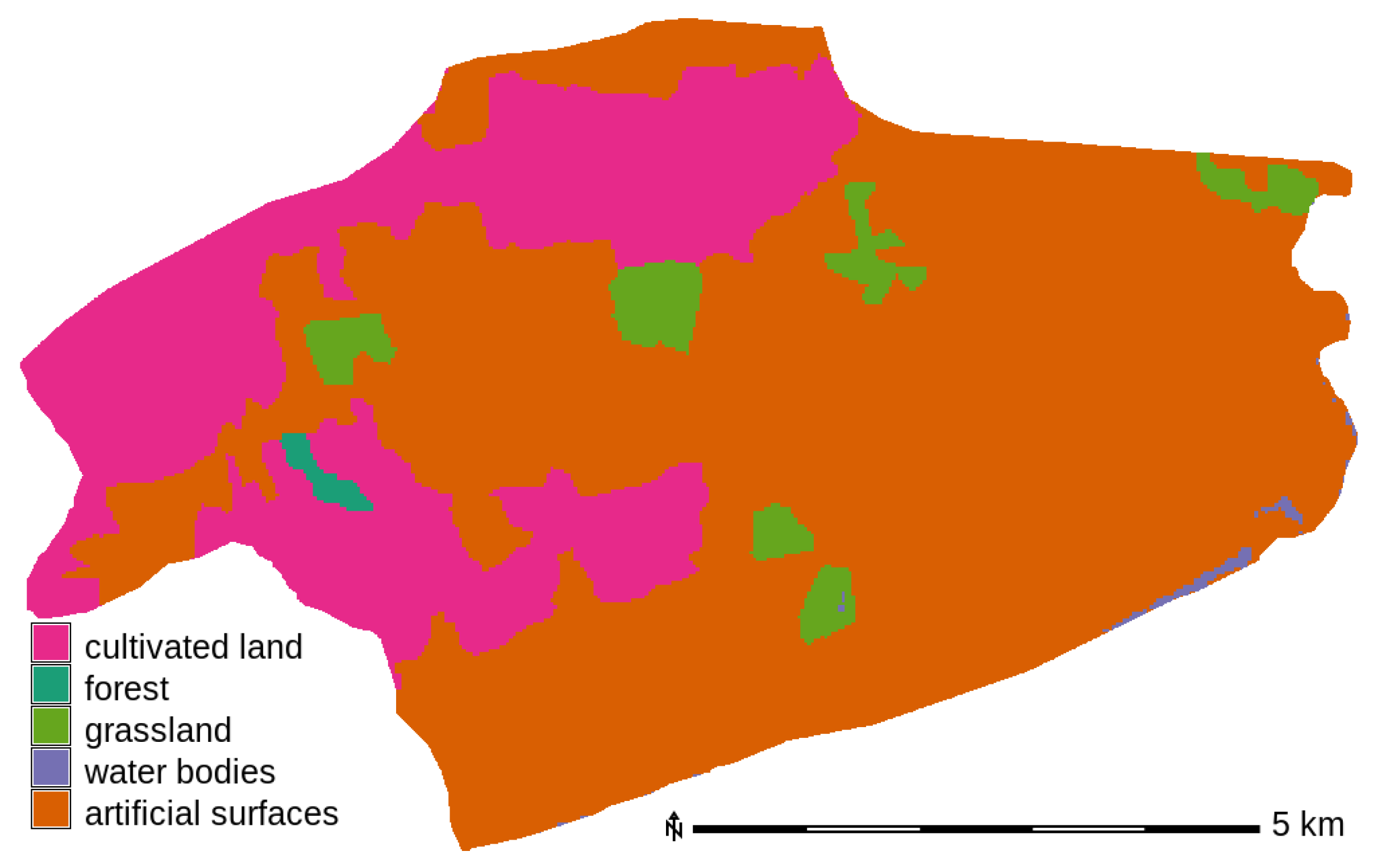
Manning’s n friction map is created using the Global Land Cover (GLC30) map from the National Geomatics Center of China [27]. Figure 4 shows the map of the repartition of the land cover classes over the study area. Typical values of n from the literature are assigned for each cell according to its class [28]. Table 4 shows the relation between the land cover classes and Manning’s n values proposed by Chow [28].
2.2.5. Drainage
The drainage of the city of Hull is entirely pumped because of the topographic situation of the urban area [21]. The drainage of the study area was carried out by the combined action of the following pumping stations that worked continuously during the event [21]:
- West Hull pumping station (capacity 32 ), draining the whole study area plus a smaller part of the city north of it.
- Saltend Waste Water Treatment Work (outflow 22 ), treating most of Hull, including the study area.
Yu and Coulthard [1] mentioned drainage capacity values for Hull of 70 for the urban area and 15 for the rural areas. Applying 70 of drainage capacity to the urbanized part of the study area (see Figure 4) represents an average flow of . This value is coherent with the installed pumping capacity described above. Therefore, we created a drainage capacity map using the values from Yu and Coulthard [1] on the urban and non-urban areas defined by the GLC30 map (See Figure 4). The artificial surfaces have been assigned a value of and the remaining areas .
2.2.6. Infiltration
Coulthard and Frostick [21] estimate that the soil was saturated due to the important rainfall prior to the studied event. Therefore, we consider that the infiltration could range from zero (where no infiltration at all happens) to a value depending on the hydraulic conductivity of the soil. We estimated the possible hydraulic conductivity over the study area with the help of the global soil database SoilGrids250m [29]. First, we calculate the average clay and sand values in the top 60 cm of soil. Then, we use the resulting maps to classify the soil according to texture definitions from the United States Department of Agriculture (USDA). Finally, we relate the texture classes with typical values obtained from experiments [30]. Table 5 displays the values obtained by this methodology. The average hydraulic conductivity estimated in the study area is .
We acknowledge the uncertainty of the method used to estimate the conductivity, especially in an urban environment, and use uniform values of infiltration for model calibration. We consider the infiltration to be equal to the hydraulic conductivity, which is consistent with the Green–Ampt equation when used in saturated soils. Therefore, the infiltration values we use for the model calibration are 0 to 5 with a 1 step.
2.2.7. Precipitation
For the precipitation, we compare two sources of information. The first one is the measurement from an uncalibrated rain gauge at the University of Hull [1]. Its temporal resolution is 1 , and it is considered uniform in space. The second one is a time series of raster maps reconstructed using various rain gauges and a meteorological radar. Although weather radar provides spatial rainfall information, it fails to estimate the correct intensity, partly because it may be affected by different sources of errors. On the other hand, rain gauges can measure the point rainfall intensities more accurately, but are unable to provide information on the spatial rainfall distribution. Merging the two sources of rainfall data is recognised to improve the estimates [19,31,32,33,34]. The selected radar-gauge merging method is Kriging with External Drift (KED) [35,36]. KED assumes the mean of the process (drift) as a linear function of external covariates. In this case, the only considered covariate is the radar rainfall.
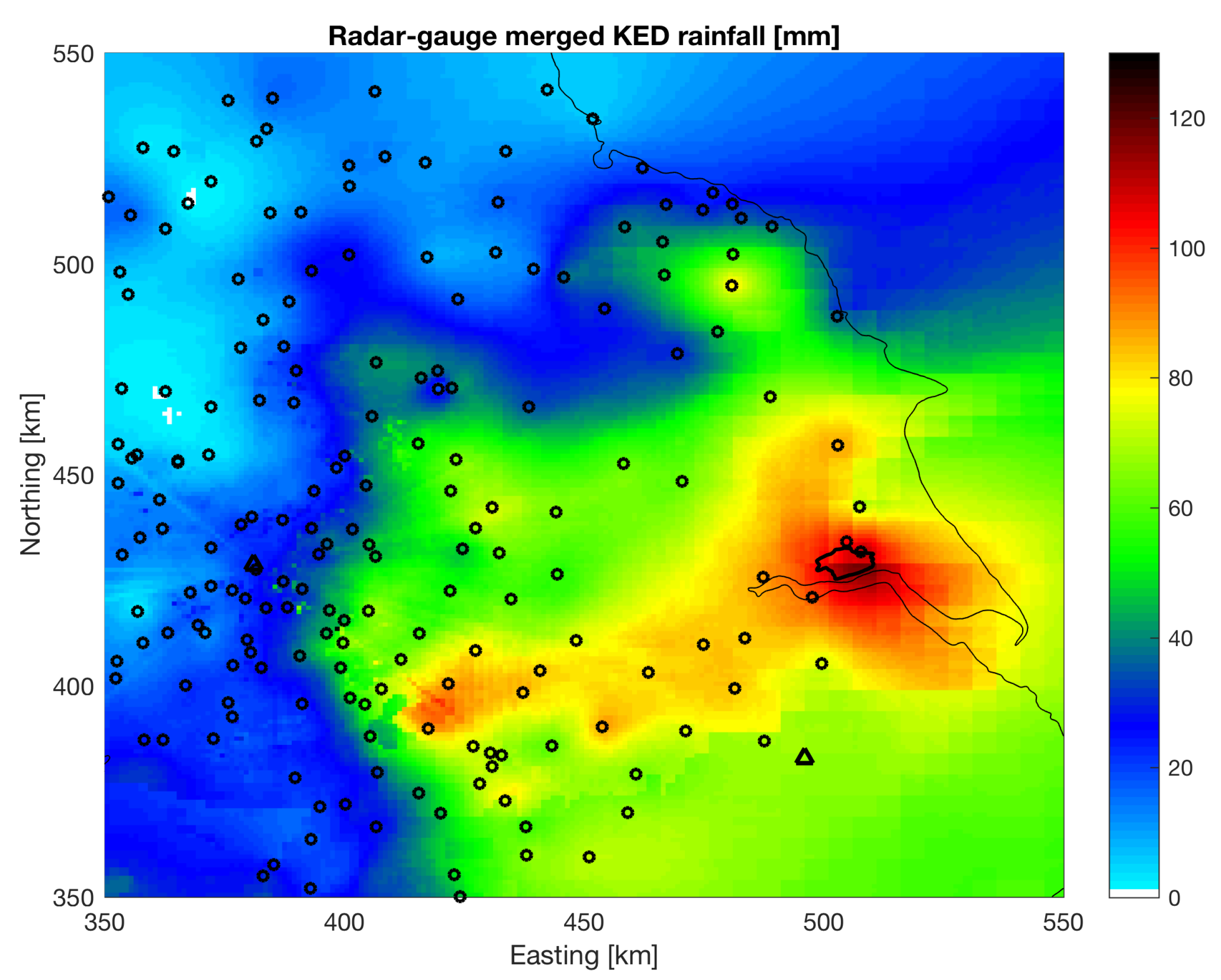
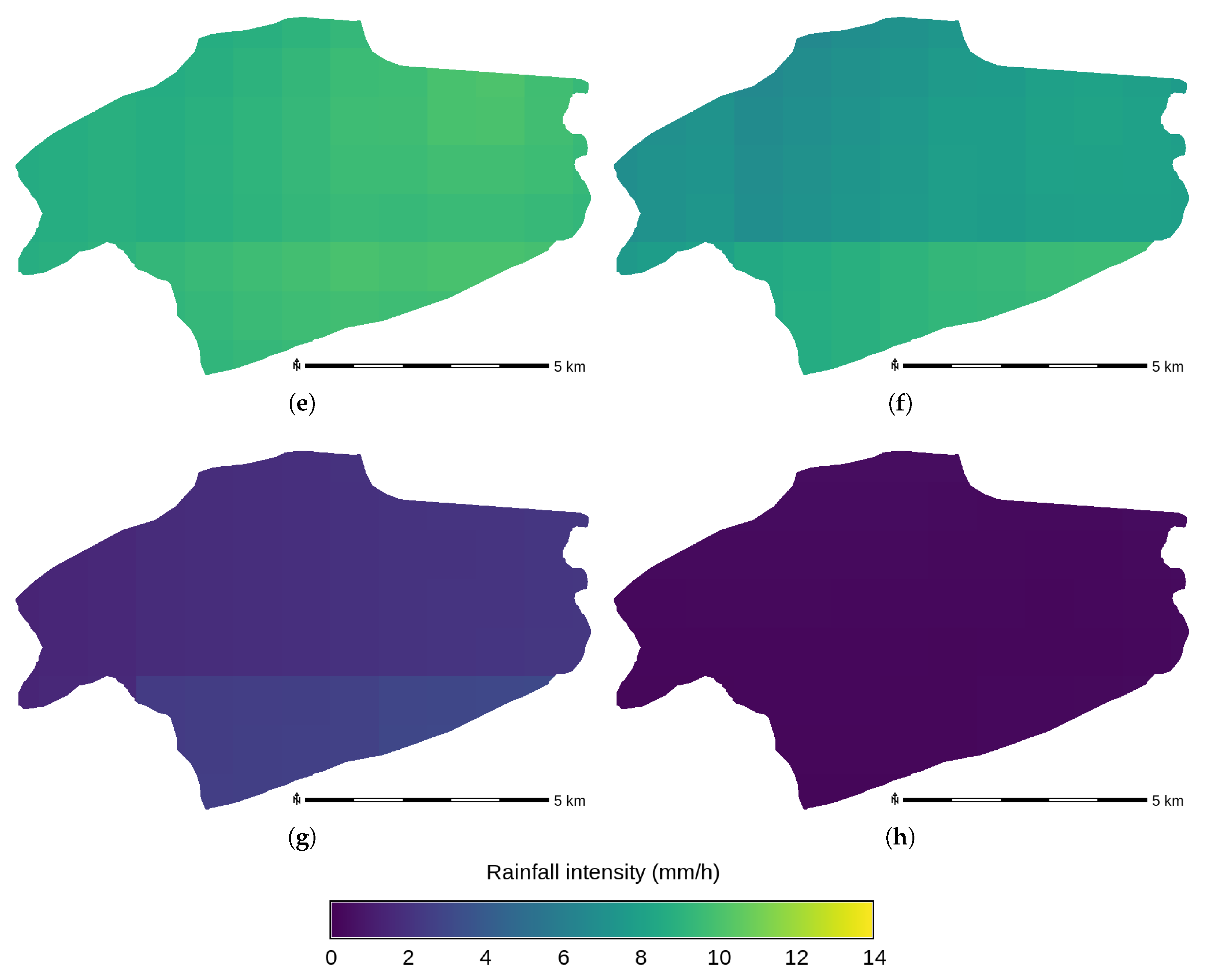
For this event, we use the weather radar rainfall composite product from the U.K. Met Office at 1 km and 5 spatial and temporal resolutions [37] and a series of rain gauges from the EA to create the raster time series using KED. The radar rainfall product has been quality-controlled by the U.K. Met Office, and it has been corrected for well-known sources of error in radar rainfall [38]. Note that the urban area was mainly covered by the Hameldon Hill radar located more than 100 km towards the west of the urban area. Figure 5 shows the map of accumulated precipitation together with the locations of the weather radar and rain gauges. Due to the distance of the radar from Hull, the actual radar rainfall spatial resolution above the study area is around 5 km. Furthermore, the radar rainfall had gaps in data during this event, and therefore, the missing time periods were interpolated using a nowcasting model [39]. Unfortunately, some of the missing periods occurred during the time of heavy precipitation falling on the study area. The spatial resolution of the resulting rainfall field is 1 km. The radar rainfall scans were accumulated to produce a temporal resolution of 1 h, similar to the uniform rainfall. Figure 6 shows the evolution in time of the rainfall field generated by KED. Note that some time steps shown in Figure 6 show a KED spatial rainfall resolution of 1 km due to the fact that the radar-gauge KED merging was performed at 1 km resolution and also because the nowcasting model to interpolate the missing time periods also runs at 1 km.
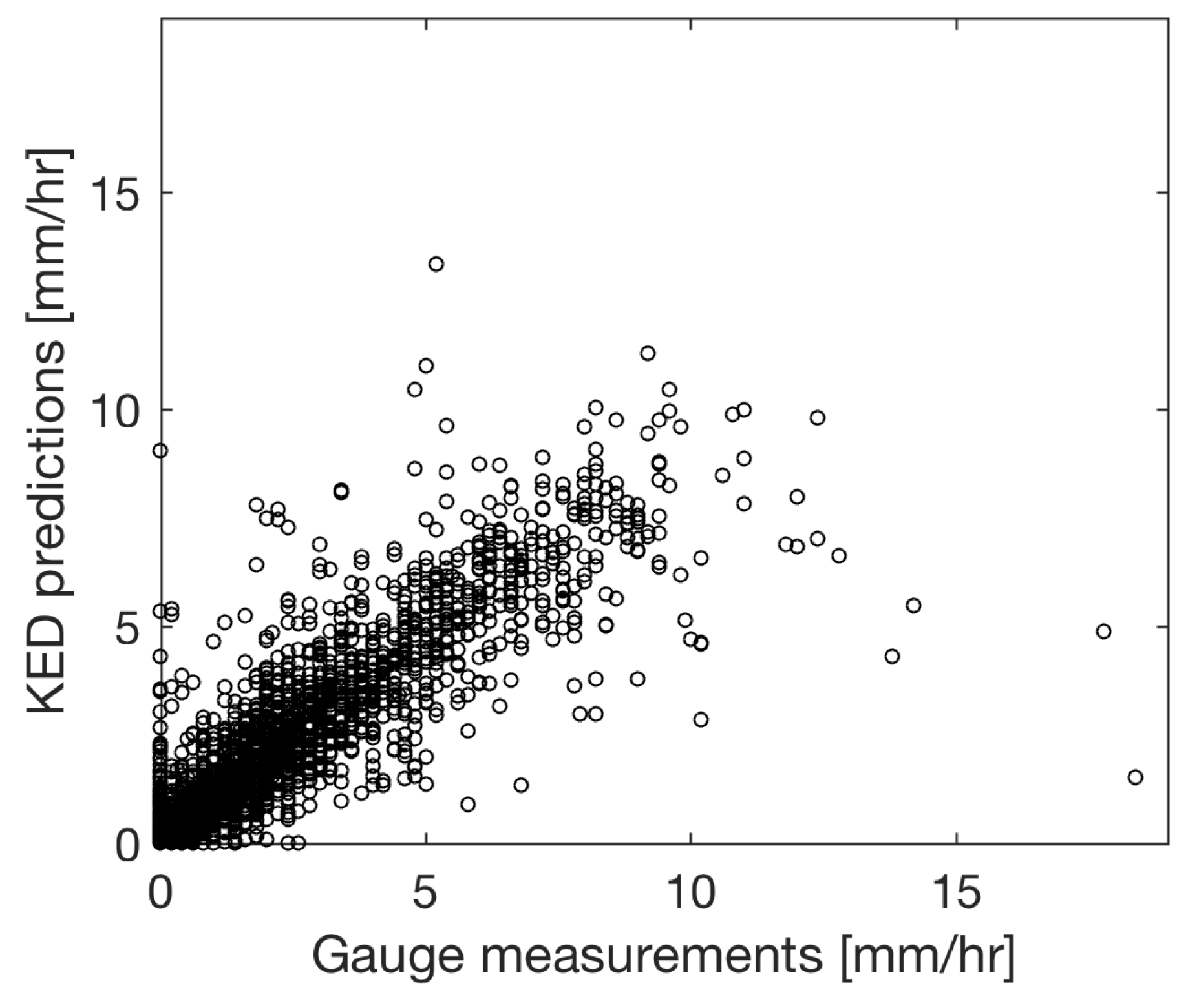
The performance of the KED rainfall predictions was evaluated by using the Leave-One-Out Cross-Validation (LOOCV) method. The method consists of computing the KED rainfall fields by leaving one of the rain gauges out for validation, then repeating the process with another rain gauge, and so on, until all the rain gauges are cross-validated. The results are shown in Figure 7. The KED performance gives a normalised error of 30% , Root Mean Square Error (RMSE) of , bias of 1.0 (i.e., unbiased), Mean Absolute Error (MAE) of and Nash–Sutcliffe efficiency of 0.8.
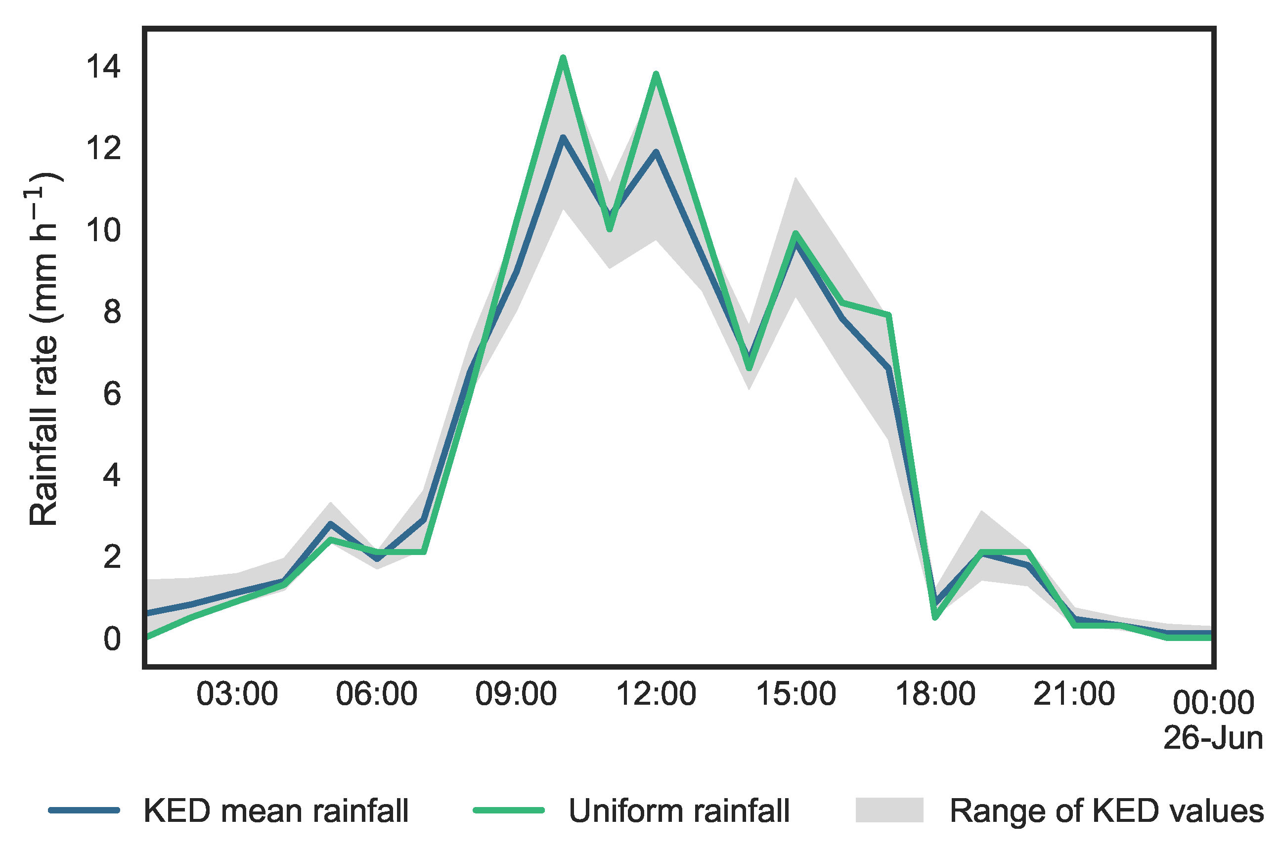
The mean hyetographs of each rainfall, averaged above the urban area, are compared in Figure 8. The peak intensity of the KED rainfall is lower than the uniform rainfall, but at lower intensity, the KED rainfall shows higher values. On the same figure is represented the range of intensity values that are present in the raster rainfall field obtained by KED. This allows for a better understanding of the spatial variability of the rainfall during this event. The spatial variability of the KED rainfall is higher when the intensity is higher. The precipitated volumes during the event are and for the uniform rainfall and the KED rainfall, respectively.
3. Results
We first calibrate the model with the uniform rainfall using the infiltration as a calibration value. Secondly, we run an additional simulation using the calibrated values and the KED rainfall. We then compare the results obtained with the KED rainfall to those obtained with the uniform rainfall. To do so, we subject the results to two types of analysis: a qualitative one and a quantitative one.
3.1. Model Calibration
Since this case is not sensitive to friction [1], we select only the infiltration as a calibration value. As mentioned in Section 2.2.6, we use the uniform infiltration values of 0, 1, 2, 3, 4 and 5 . For this process of calibration, we use the uniform rainfall. We calibrate the model using the identified flood extents as references. We have two maps of flood extent with significant differences between them (see Section 2.2.3). Therefore, we use those two maps plus a union of those two extents as references against which the model results will be compared.
In order to compare the computed flooded areas to the observed ones, we classify each cell as flooded or dry by applying a water depth threshold on the computed water depth. There is no definite literature on the value of this threshold, and it is mostly arbitrary [40]. Therefore, we use a series of 31 values from 0.5 cm to 35 cm distributed with a 1 cm step. Logically, the generated binary maps shows a larger extent of inundation when the threshold is lower and a smaller extent with a higher threshold. The first step to compare those generated maps to the observed extent maps is to classify the results in a contingency table (see Table 6). This contingency table is then used to calculate the Critical Success Index (CSI) [40], a skill evaluation score commonly used in hydrology (e.g., [41,42]). This score is calculated using . The combination of entry data that obtain the highest CSI will be used as a reference simulation to compare the two rainfall data.
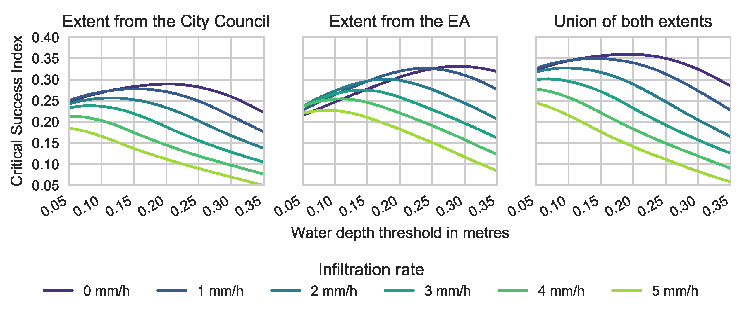
The computed values of CSI obtained of the six simulations are shown in Figure 9. Each individual observed extent gives a lower value of CSI than the union of both extents. In that latter case, the highest value of CSI is obtained without any infiltration and at a water depth threshold of 20 cm. The highest CSI value is 0.36. Therefore, we retain the following calibration values:
- Union of observed flooded extents as the “real-world” reference.
- No infiltration.
- Water depth threshold of 20 cm.
3.2. Qualitative Analysis
During the event, the water accumulates in the lower part of the domain, which is also the most urbanised. Figure 10 compares the computed maximal water levels with the observed extents. It shows that the model is able to identify the main flooded area observed by the two collecting entities, at the centre of the domain. For the other inundated parts, the comparison is more difficult because of the discrepancies between the observations of the EA and the HCC.
Some differences in computed water level occur between the simulation using the KED rainfall and the one using uniform rainfall. Those differences are not easily noticed in Figure 10. Figure 11 allows an easier representation of those differences in maximal water depths. It could be noted that water levels obtained using KED are consistently lower than those using the uniform rainfall. This could be related to the smaller precipitated volume of the KED rainfall (see Section 2.2.7). The discrepancies are mostly between 5 cm to 10 cm and are larger going eastward. In more limited areas, the differences reach 15 cm. Those higher differences in the eastern part of the domain might be due to the inundation being mostly due to the overland flow coming from the upstream areas on the west, and not from the local precipitation. The observed difference might therefore be due to the flood wave not reaching that far east when the precipitated volume is lower.
3.3. Quantitative Analysis
In order to compare the results obtained with the uniform rainfall and those obtained with KED, we calculate for each simulation result the CSI, total flooded area and percentage of the computational domain that is flooded. Those calculations are first done with maximal water depths map, then we proceed to do a similar analysis with the evolution in time of those values along the simulation. For all those analyses, we employ the values determined by the model calibration (see Section 3.1).
First, we compare the maximal water depth maps obtained by the two rainfalls. Table 7 shows the results of this analysis. The surface flooded is lower when using the KED rainfall. This is explained by the lower accumulated precipitated volume of the KED rainfall compared with the uniform rainfall (see Section 2.2.7). Regarding the skill, the CSI obtained with each of the rainfalls is quite weak, with values lower than 0.4. However, the uniform rainfall results in a CSI slightly higher than the KED, with 0.36 against 0.35.
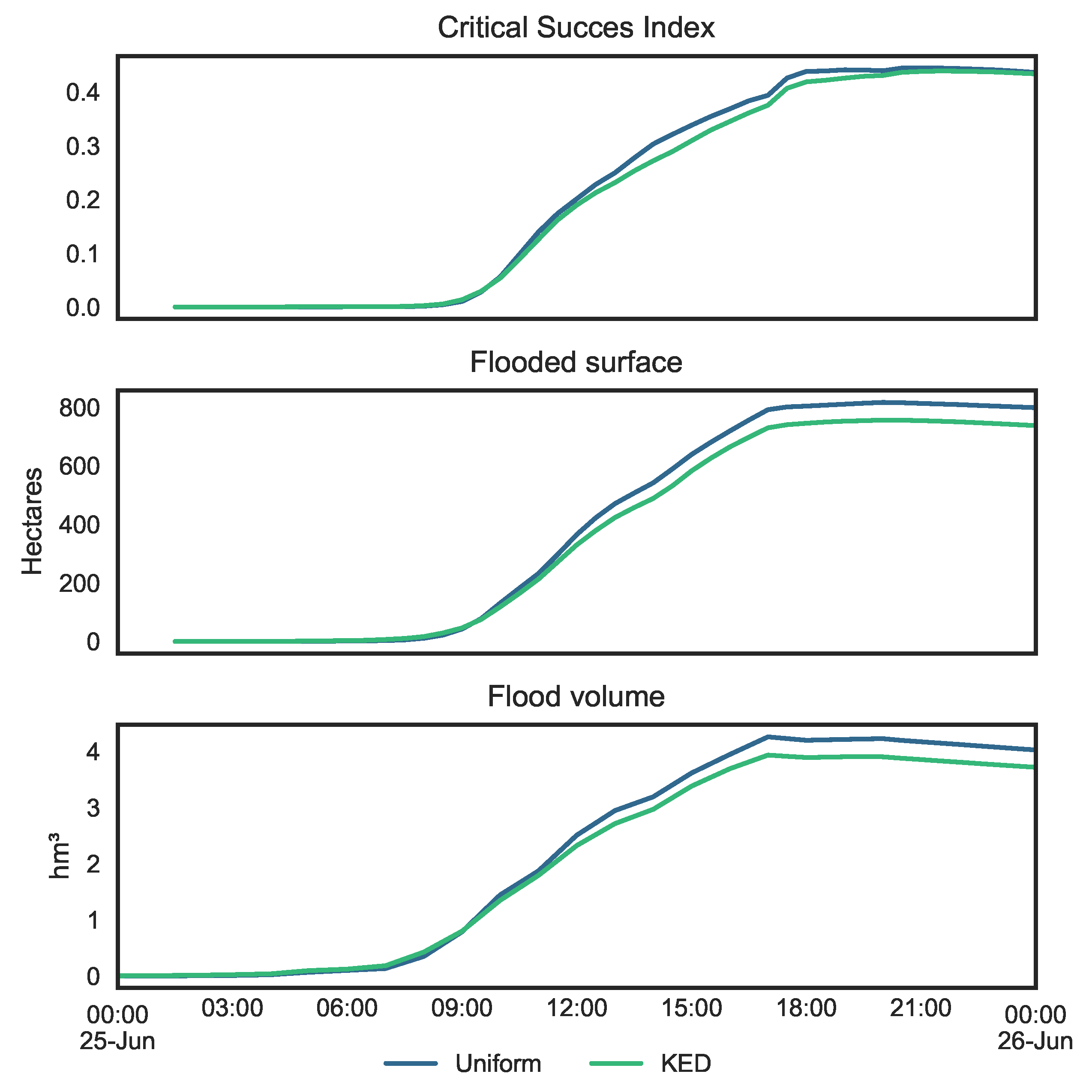
Second, we examine the evolution in time of the flooded area, the flood volume and the CSI. Figure 12 shows the plots in time of those values obtained with the two different rainfalls. We can notice that the rate of change of all three values is logically affected by the intensity of the rainfalls (see Figure 8), with the steepest increase being between 07:00 and 17:00. The flooded volumes obtained with the two rainfalls reach their highest values at the same time, 17:00. However, the flooded area continues to grow afterwards, with a peak occurring at 20:00. This is likely due to the spreading of the inundation continuing at smaller depths, resulting in a growing flooded area, even though the volume is getting smaller. Considering the CSI, the values obtained with the uniform rainfall are higher than those obtained with KED for most of the simulation. However, the difference becomes much smaller as the water level stabilizes. With the uniform rainfall, the CSI peaks at 21:00 with a value of 0.445, while with the KED, it peaks at 21:30 with a value of 0.439. At the end of the simulation, the CSI values for uniform and KED rainfall are 0.436 and 0.434, respectively. Furthermore, it is notable that the maximum CSI obtained during this exercise is higher than that obtained with the maximum water level (see Table 7). We can explain that by the fact that the maximal water depth map includes the water channels that form in the more hilly west part of the basin (see Figure 10). This creates flooded cells in those areas that are not reported as flooded by any of the two authorities, inducing a lower skill for both of the tested rainfalls. On the other hand, those channels dry out when the rain stops, which induces a higher CSI when calculating it using maps of instantaneous water depths. This fact is reflected in the differences observed between the flooded areas calculated by snapshot water depths (816 ha) to the one obtained with the maximal water depths (935 ha; see Figure 8).
4. Discussion and Conclusions
In this paper, we compared the computer simulation results obtained by the use of uniform and KED rainfall to the observed inundation extents of the historical event of June 2007 in Hull, U.K. Although the spatial variability of the KED rainfall is slight (see Figure 6), differences appear. For instance, the flooded area obtained with the KED rainfall is 8% lower than the one obtained with the uniform rainfall (see Table 7). This is due to a lower precipitated volume and, in turn, a lower flooded volume when using the KED. However, those differences in flood volume and inundated areas do not reflect in the skill scores obtained by the two rainfalls when comparing the computed flood extents to the observations of actual affected zones. Indeed, the differences in CSI for those two rainfalls are not sufficient to be conclusive and should not be used to assert the superiority of one rainfall datum against the other.
Two factors inherent to this specific event might influence those results. First, the observations of flooded zones are unlikely to accurately identify the affected areas (see Section 2.2.3). This uncertainty in the observations reduces the reliability of the calibration and evaluation processes. Second, the available radar data for this event come from equipment rather far from the study area. This results in a practical spatial resolution of around 5 km. Furthermore, there were missing time periods in the radar data that needed to be filled using nowcasting interpolation before preforming the KED radar-gauge merging.
Unfortunately, uncertain or scarce observations are common during extreme flood events (e.g., [43]). Maps of observed flooding are especially difficult to obtain in urban areas due to the short time scale of their occurrence (usually a few hours). Few urban areas are instrumented, and remote-sensing techniques might be of limited use [7]. In addition to the relatively low revisit time of spacecraft carrying high-resolution instruments, some technologies like multi-spectral imagery are seldom usable because of the cloud cover during or immediately after the precipitation event. In that sense, in spite of the limitations of the available data, the present case study can be considered data-rich because it includes both non-uniform rainfall data and observations of the affected areas.
Therefore, this study is a step forward in the direction of having a better understanding of the impact of the spatial variation of rainfall on the flood modelling of historical events. It shows that even with limited and uncertain data, the incorporation of the spatial variability of rainfall does have an impact on the numerical results. We can mention that should another flooding event occur in the same area, the definition of the rainfall data might improve due to the inclusion of the data of the Ingham radar, for the south of the study area (see Figure 5), which in turn might improve the reproduction of the inundation. Each event is different, and the relative size of the precipitation compared to the study area is to be considered. In urban areas of limited extent like Hull, more localized events like convective precipitations might require even more consideration of the spatial component of rainfall. More similar studies should be carried out in the future that will tackle the subject with other types of events and study areas, including different types of meteorological events, topography and land use.
Acknowledgments
The authors would like to thank the U.K. Met Office (radar rainfall requests to Met Office [38]) and the Environment Agency (rain gauge data requests at http://environment-agency.gov.uk/) for providing some of the datasets used in this study. We thank Dapeng Yu from Loughborough University for kindly providing the DEM, the maps of observed flooded areas and the rain gauge records at the University of Hull. Laurent Courty is supported by the Coordination of Postgraduate Studies of the Universidad Nacional Autónoma de México through a full doctoral scholarship. Adrián Pedrozo-Acuña and Laurent Courty thankfully acknowledge the support from the Secretaría de Ciencia Tecnología e Innovación de la Ciudad de México through the project number SECITI/113/2017 “Smart Water, smart city”.
Author Contributions
Adrián Pedrozo-Acuña and Laurent Courty designed the study. Laurent Courty performed the experiments and created most of the figures. Miguel Rico-Ramirez generated the KED rainfall field and Figure 5 and Figure 7. All authors participated in the interpretation of the results and the redaction of the manuscript.
Conflicts of Interest
The authors declare no conflict of interest.
Abbreviations
The following abbreviations are used in this manuscript:
| CSI | Critical Success Index |
| DEM | Digital Elevation Model |
| EA | Environment Agency of the United Kingdom |
| GIS | Geographical Information System |
| GLC30 | Global Land Cover |
| GRASS | Geographic Resources Analysis Support System |
| HCC | Hull City Council |
| KED | Kriging with External Drift |
| LiDAR | Light Detection And Ranging |
| LOOCV | Leave-One-Out Cross-Validation |
| MAE | Mean Absolute Error |
| RMSE | Root Mean Square Error |
| SVE | Saint–Venant Equations |
| USDA | United States Department of Agriculture |
References
- Yu, D.; Coulthard, T.J. Evaluating the importance of catchment hydrological parameters for urban surface water flood modelling using a simple hydro-inundation model. J. Hydrol. 2015, 524, 385–400. [Google Scholar] [CrossRef] [Green Version]
- Courty, L.G.; Pedrozo-Acuña, A.; Bates, P.D. Itzï (version 17.1): An open-source, distributed GIS model for dynamic flood simulation. Geosci. Model Dev. 2017, 10, 1835–1847. [Google Scholar] [CrossRef]
- Hirabayashi, Y.; Mahendran, R.; Koirala, S.; Konoshima, L.; Yamazaki, D.; Watanabe, S.; Kim, H.; Kanae, S. Global flood risk under climate change. Nat. Clim. Chang. 2013, 3, 816–821. [Google Scholar] [CrossRef]
- Vojinović, Z.; Abbott, M.B. Flood Risk and Social Justice: From Quantitative to Qualitative Flood Risk Assessment and Mitigation; IWA Publishing: London, UK, 2012; p. 563. [Google Scholar]
- Hunter, N.M.; Bates, P.D.; Neelz, S.; Pender, G.; Villanueva, I.; Wright, N.G.; Liang, D.; Falconer, R.A.; Lin, B.; Waller, S.; et al. Benchmarking 2D hydraulic models for urban flooding. Proc. ICE Water Manag. 2008, 161, 13–30. [Google Scholar] [CrossRef] [Green Version]
- Zevenbergen, C.; Cashman, A.C.; Evelpidou, N.; Pasche, E.; Garvin, S.; Ashley, R. Urban Flood Management; CRC Press: Boca Raton, FL, USA, 2010. [Google Scholar]
- Di Baldassarre, G. Data sources. In Floods in a Changing Climate: Inundation Modelling; Cambridge University Press: Cambridge, UK, 2012; pp. 33–42. [Google Scholar]
- Cristiano, E.; ten Veldhuis, M.C.; van de Giesen, N. Spatial and temporal variability of rainfall and their effects on hydrological response in urban areas—A review. Hydrol. Earth Syst. Sci. 2017, 21, 3859–3878. [Google Scholar] [CrossRef]
- Arnaud, P.; Bouvier, C.; Cisneros, L.; Dominguez, R. Influence of rainfall spatial variability on flood prediction. J. Hydrol. 2002, 260, 216–230. [Google Scholar] [CrossRef]
- Segond, M.L.; Wheater, H.S.; Onof, C. The significance of spatial rainfall representation for flood runoff estimation: A numerical evaluation based on the Lee catchment, UK. J. Hydrol. 2007, 347, 116–131. [Google Scholar] [CrossRef]
- Gires, A.; Onof, C.; Maksimovic, C.; Schertzer, D.; Tchiguirinskaia, I.; Simoes, N. Quantifying the impact of small scale unmeasured rainfall variability on urban runoff through multifractal downscaling: A case study. J. Hydrol. 2012, 442–443, 117–128. [Google Scholar] [CrossRef]
- Bruni, G.; Reinoso, R.; Van De Giesen, N.C.; Clemens, F.H.L.R.; Ten Veldhuis, J.A.E. On the sensitivity of urban hydrodynamic modelling to rainfall spatial and temporal resolution. Hydrol. Earth Syst. Sci. 2015, 19, 691–709. [Google Scholar] [CrossRef]
- Rico-Ramirez, M.; Liguori, S.; Schellart, A. Quantifying radar-rainfall uncertainties in urban drainage flow modelling. J. Hydrol. 2015, 528, 17–28. [Google Scholar] [CrossRef]
- Seo, D.J. Real-time estimation of rainfall fields using radar rainfall and rain gage data. J. Hydrol. 1998, 208, 37–52. [Google Scholar] [CrossRef]
- Nesbitt, S.W.; Anders, A.M. Very high resolution precipitation climatologies from the Tropical Rainfall Measuring Mission precipitation radar. Geophys. Res. Lett. 2009, 36. [Google Scholar] [CrossRef]
- Smith, J.A.; Baeck, M.L.; Meierdiercks, K.L.; Miller, A.J.; Krajewski, W.F. Radar rainfall estimation for flash flood forecasting in small urban watersheds. Adv. Water Resour. 2007, 30, 2087–2097. [Google Scholar] [CrossRef]
- Smith, J.A.; Krajewski, W.F. A modeling study of rainfall rate-reflectivity relationships. Water Resour. Res. 1993, 29, 2505–2514. [Google Scholar] [CrossRef]
- Ercan, M.B.; Goodall, J.L. Estimating Watershed-Scale Precipitation by Combining Gauge- and Radar-Derived Observations. J. Hydrol. Eng. 2013, 18, 983–994. [Google Scholar] [CrossRef]
- Goudenhoofdt, E.; Delobbe, L. Evaluation of radar-gauge merging methods for quantitative precipitation estimates. Hydrol. Earth Syst. Sci. 2009, 13, 195–203. [Google Scholar] [CrossRef]
- Velasco-Forero, C.A.; Sempere-Torres, D.; Cassiraga, E.F.; Jaime Gómez-Hernández, J. A non-parametric automatic blending methodology to estimate rainfall fields from rain gauge and radar data. Adv. Water Resour. 2009, 32, 986–1002. [Google Scholar] [CrossRef]
- Coulthard, T.; Frostick, L. The Hull floods of 2007: Implications for the governance and management of urban drainage systems. J. Flood Risk Manag. 2010, 3, 223–231. [Google Scholar] [CrossRef]
- Bates, P.D.; Horritt, M.S.; Fewtrell, T.J. A simple inertial formulation of the shallow water equations for efficient two-dimensional flood inundation modelling. J. Hydrol. 2010, 387, 33–45. [Google Scholar] [CrossRef]
- De Almeida, G.A.M.; Bates, P.D.; Freer, J.E.; Souvignet, M. Improving the stability of a simple formulation of the shallow water equations for 2-D flood modeling. Water Resour. Res. 2012, 48, 1–14. [Google Scholar] [CrossRef]
- De Almeida, G.A.M.; Bates, P.D. Applicability of the local inertial approximation of the shallow water equations to flood modeling. Water Resour. Res. 2013, 49, 4833–4844. [Google Scholar] [CrossRef]
- Neteler, M.; Bowman, M.H.; Landa, M.; Metz, M. GRASS GIS: A multi-purpose open source GIS. Environ. Model. Softw. 2012, 31, 124–130. [Google Scholar] [CrossRef]
- Klein Tank, A.M.G.; Wijngaard, J.B.; Können, G.P.; Böhm, R.; Demarée, G.; Gocheva, A.; Mileta, M.; Pashiardis, S.; Hejkrlik, L.; Kern-Hansen, C.; et al. Daily dataset of 20th-century surface air temperature and precipitation series for the European Climate Assessment. Int. J. Climatol. 2002, 22, 1441–1453. [Google Scholar] [CrossRef]
- Chen, J.; Chen, J.; Liao, A.; Cao, X.; Chen, L.; Chen, X.; He, C.; Han, G.; Peng, S.; Lu, M.; et al. Global land cover mapping at 30 m resolution: A POK-based operational approach. ISPRS J. Photogramm. Remote Sens. 2014, 103, 7–27. [Google Scholar] [CrossRef]
- Chow, V.T. Open Channel Hydraulics; McGraw-Hill Book Company, Inc.: New York, NY, USA, 1959. [Google Scholar]
- Hengl, T.; Mendes de Jesus, J.; Heuvelink, G.B.M.; Gonzalez, M.R.; Kilibarda, M.; Blagotí, A.; Shangguan, W.; Wright, M.N.; Geng, X.; Bauer-Marschallinger, B.; et al. SoilGrids250m: Global Gridded Soil Information Based on Machine Learning. PLoS ONE 2017, 12, e0169748. [Google Scholar] [CrossRef] [PubMed]
- Rawls, W.J.; Brakensiek, D.L.; Miller, N. Green-Ampt infiltration parameters from soils data. J. Hydraul. Eng. 1983, 109, 62–70. [Google Scholar]
- Haberlandt, U. Geostatistical interpolation of hourly precipitation from rain gauges and radar for a large-scale extreme rainfall event. J. Hydrol. 2007, 332, 144–157. [Google Scholar] [CrossRef]
- Jewell, S.A.; Gaussiat, N. An assessment of kriging-based rain-gauge-radar merging techniques. Q. J. R. Meteorol. Soc. 2015, 141, 2300–2313. [Google Scholar] [CrossRef]
- Schuurmans, J.M.; Bierkens, M.F.P.; Pebesma, E.J.; Uijlenhoet, R.; Schuurmans, J.M.; Bierkens, M.F.P.; Pebesma, E.J.; Uijlenhoet, R. Automatic Prediction of High-Resolution Daily Rainfall Fields for Multiple Extents: The Potential of Operational Radar. J. Hydrometeorol. 2007, 8, 1204–1224. [Google Scholar] [CrossRef]
- Wilson, J.W. Integration of Radar and Raingage Data for Improved Rainfall Measurement. J. Appl. Meteorol. 1970, 9, 489–497. [Google Scholar] [CrossRef]
- Chiles, J.P.; Delfiner, P. Geostatistics: Modeling Spatial Uncertainty; John Wiley & Sons: Hoboken, NJ, USA, 2012; p. 726. [Google Scholar]
- Cressie, N. Statistics for Spatial Data, Revised ed.; John Wiley & Sons: Hoboken, NJ, USA, 2015; p. 928. [Google Scholar]
- Harrison, D.L.; Scovell, R.W.; Kitchen, M. High-resolution precipitation estimates for hydrological uses. Proc. Inst. Civ. Eng. Water Manag. 2009, 162, 125–135. [Google Scholar] [CrossRef]
- Met Office. 1 km Resolution UK Composite Rainfall Data from the Met Office Nimrod System; NCAS British Atmospheric Data Centre: Didcot, UK, 2003. [Google Scholar]
- Liguori, S.; Rico-Ramirez, M.A. A review of current approaches to radar-based quantitative precipitation forecasts. Int. J. River Basin Manag. 2014, 12, 391–402. [Google Scholar] [CrossRef]
- Wilks, D. Forecast Verification. In Statistical Methods in the Atmospheric Sciences; Elsevier: Amsterdam, The Netherlands, 2011; pp. 301–394. [Google Scholar]
- Horritt, M.S.; Bates, P.D. Evaluation of 1D and 2D numerical models for predicting river flood inundation. J. Hydrol. 2002, 268, 87–99. [Google Scholar] [CrossRef]
- Cook, A.; Merwade, V. Effect of topographic data, geometric configuration and modeling approach on flood inundation mapping. J. Hydrol. 2009, 377, 131–142. [Google Scholar] [CrossRef]
- Pedrozo-Acuña, A.; Breña-Naranjo, J.A.; Domínguez-Mora, R. The hydrological setting of the 2013 floods in Mexico. Weather 2014, 69, 295–302. [Google Scholar] [CrossRef]
Figure 1.
Location of the Hull study area within Great Britain (satellite imagery Copernicus Sentinel 2016) [2].
Figure 1.
Location of the Hull study area within Great Britain (satellite imagery Copernicus Sentinel 2016) [2].
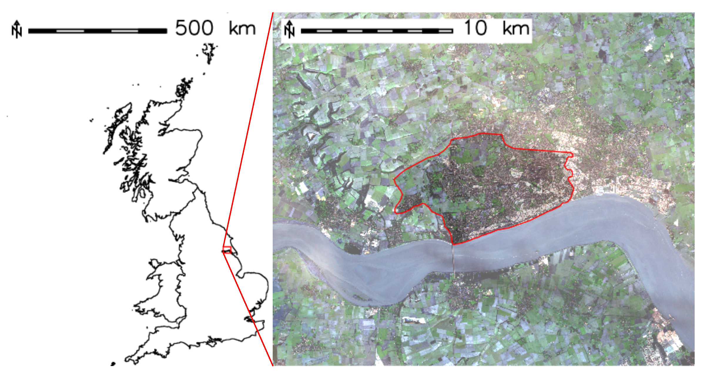
Figure 2.
Digital elevation model of the study area. Contour lines are every 5 .
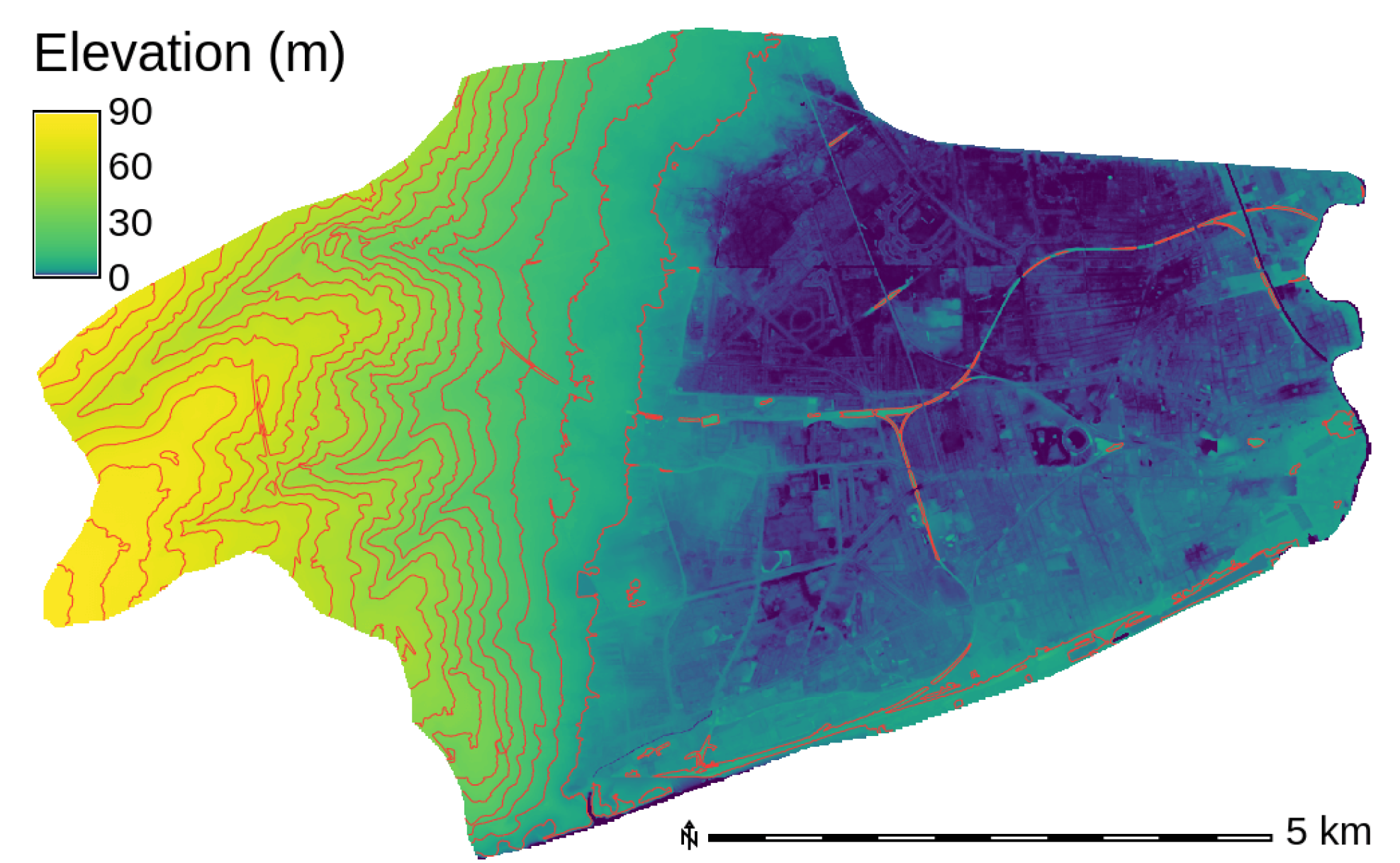
Figure 3.
Identified flooded areas. Light blue: EA only. Dark blue: HCC only. Green: intersection of both administrations.
Figure 3.
Identified flooded areas. Light blue: EA only. Dark blue: HCC only. Green: intersection of both administrations.
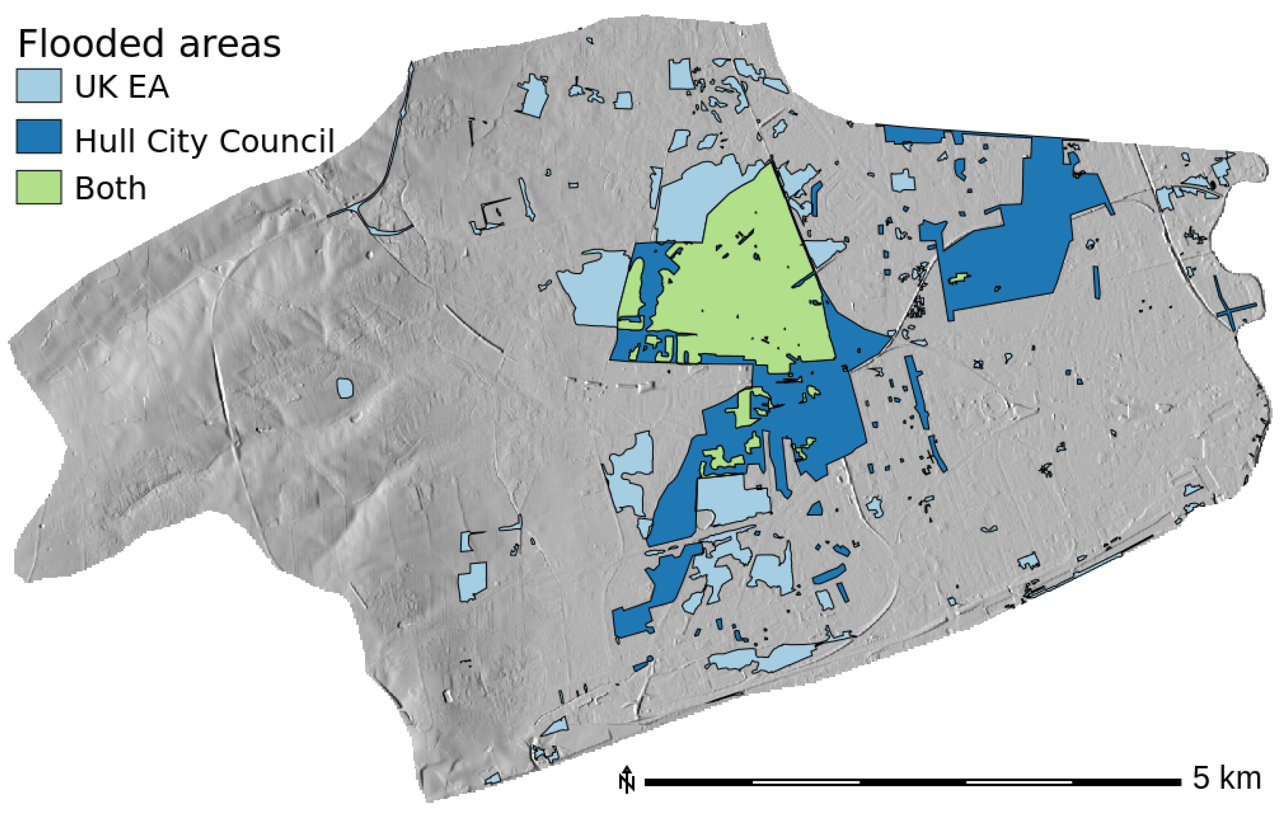
Figure 4.
Land cover classes from Global Land Cover in the study area.

Figure 5.
Accumulated rainfall obtained from Kriging with External Drift on 25 June 2007. The circles represent the rain gauges used. The triangles are the weather radars. The study site is represented by a black polygon. Please note that during this event, only the Hameldon Hill radar (located in the west of the image) was operating.

Figure 6.
Evolution of rainfall intensity above the study area obtained with Kriging with External Drift. Event of 25 June 2007. (a) 00:00–01:00; (b) 03:00–04:00; (c) 06:00–07:00; (d) 09:00–10:00; (e) 12:00–13:00; (f) 15:00–16:00; (g) 18:00–19:00; (h) 21:00–22:00.
Figure 6.
Evolution of rainfall intensity above the study area obtained with Kriging with External Drift. Event of 25 June 2007. (a) 00:00–01:00; (b) 03:00–04:00; (c) 06:00–07:00; (d) 09:00–10:00; (e) 12:00–13:00; (f) 15:00–16:00; (g) 18:00–19:00; (h) 21:00–22:00.
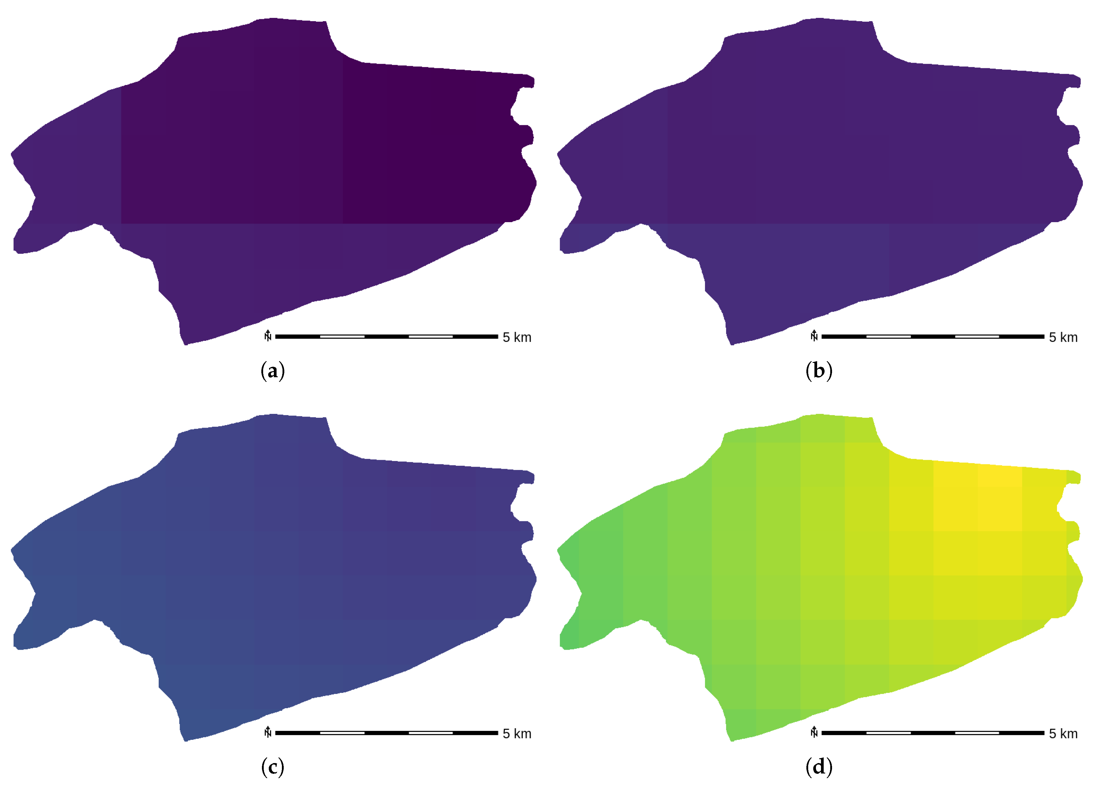

Figure 7.
KED performance using LOOCV for the event of 25 June 2007.

Figure 8.
Hyetographs of the two considered rainfalls above the study area on 25 June 2007.

Figure 9.
Values of Critical Success Index obtained during the calibration process. They are calculated using the maximal water depth maps obtained with uniform rainfall and a combination of infiltration values, water depth thresholds and observed extents.
Figure 9.
Values of Critical Success Index obtained during the calibration process. They are calculated using the maximal water depth maps obtained with uniform rainfall and a combination of infiltration values, water depth thresholds and observed extents.

Figure 10.
Comparison between observed extents and maximal computed water depths. (a) Uniform rainfall; (b) Kriging with External Drift.
Figure 10.
Comparison between observed extents and maximal computed water depths. (a) Uniform rainfall; (b) Kriging with External Drift.
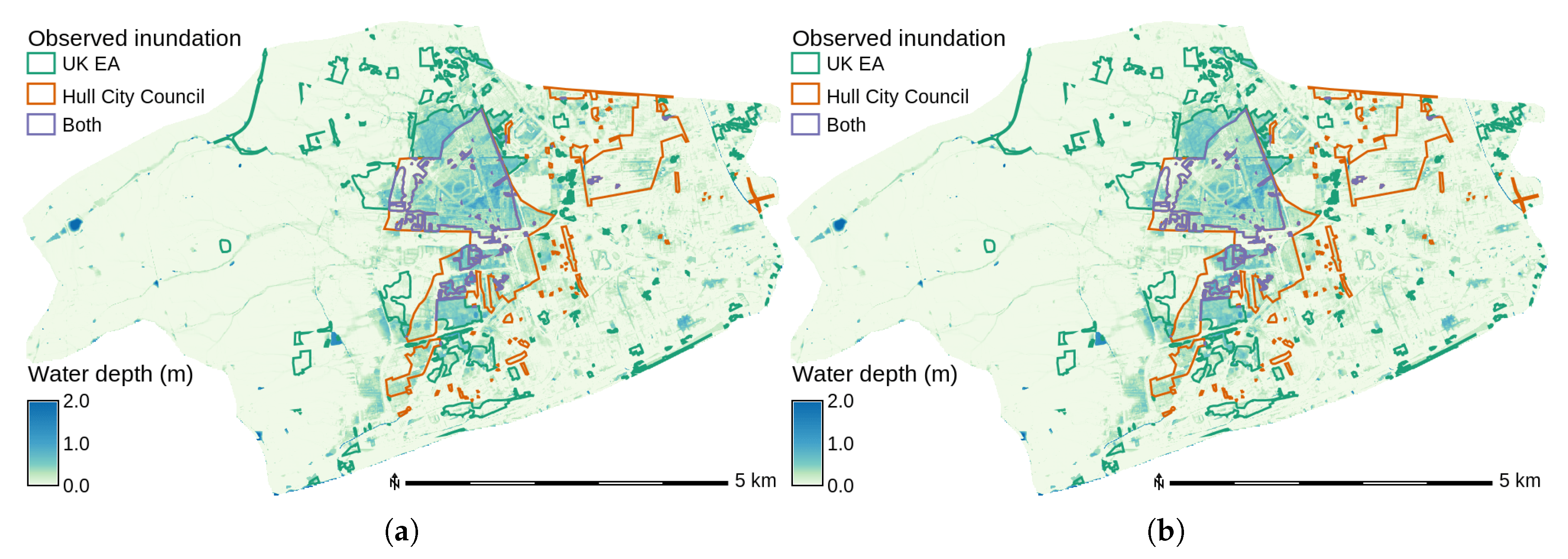
Figure 11.
Differences in maximal water depths between the results using uniform rainfall and those using Kriging with External Drift.
Figure 11.
Differences in maximal water depths between the results using uniform rainfall and those using Kriging with External Drift.
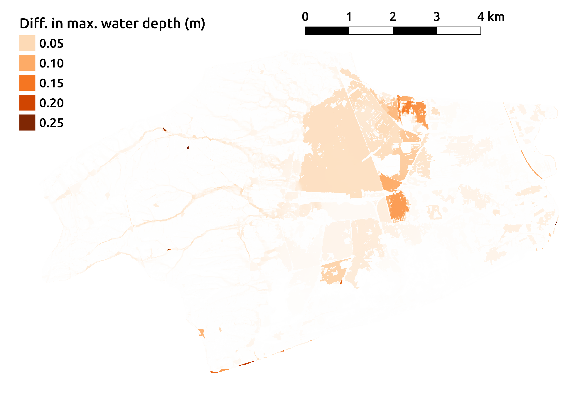
Figure 12.
Evolution in time of the flood volume, flooded surface and Critical Success Index. The flooded surface and CSI are calculated for water depths above 20 cm.
Figure 12.
Evolution in time of the flood volume, flooded surface and Critical Success Index. The flooded surface and CSI are calculated for water depths above 20 cm.

Table 1.
Features comparison between LISFLOOD-FP, FloodMap-HydroInundation2D and Itzï.
| Feature | LISFLOOD-FP | FloodMap | Itzï |
|---|---|---|---|
| Flow equation | Damped partial inertia [23,24] | Partial inertia [22] | Damped partial inertia [23,24] |
| Adaptive time step | Global | Local | Global |
| 1D river model | Yes | Yes | No |
| Infiltration model | No | Green–Ampt | Green–Ampt |
| GIS integration | Loose | Loose | Tight |
| Map time series | |||
| as input | No | No | Yes |
| Free software | No | No | Yes (GNU GPL) |
| Parallel processing | OpenMP | MPI | OpenMP |
Although Glofrim https://github.com/openearth/glofrim contains LISFLOOD-FP and is released under the GNU GPL, its README says “Please note that the downloadable LISFLOOD-FP version is not meant for further unauthorized distribution”. This places LISFLOOD-FP outside the scope of the license.
Table 2.
Modelling parameters.
| Parameter | Value |
|---|---|
| 0.7 | |
| () | 2.0 |
| 0.7 |
Table 3.
Comparison of identified flood extents.
| Collecting Entity | Area () |
|---|---|
| Environment Agency | 5.16 |
| Hull City Council | 6.18 |
| Intersection of both | 2.33 |
Table 4.
Relation between land cover classes and Manning’s n values.
| GLC30 Class | Category from Chow [28] | Manning’s n () |
|---|---|---|
| Cultivated land | Mature field crops | 0.040 |
| Forest | Cleared land with tree stumps, heavy growth of sprouts | 0.060 |
| Grassland | Pasture with short grass | 0.030 |
| Water bodies | Natural stream: clean, straight, full stage, no rifts or deep pool | 0.030 |
| Artificial surfaces | Gunite, good section | 0.019 |
Table 5.
Distribution of estimated hydraulic conductivity above the study area.
| Hydraulic Conductivity () | Surface () | Surface (%) |
|---|---|---|
| 1.00 | 18.88 | 0.30 |
| 1.50 | 654.5 | 12.0 |
| 3.50 | 4507.5 | 82.3 |
| 10.9 | 295.6 | 5.40 |
Table 6.
Contingency table used to calculate the Critical Success Index.
| Observed | |||
|---|---|---|---|
| Flooded | Not Flooded | ||
| Computed | Flooded | hits | false alarms |
| Not flooded | misses | correct negatives | |
Table 7.
Comparison of maximum flooded areas between uniform and KED rainfalls.
| Rainfall | CSI | Flooded Area (ha) | Surface Flooded (%) |
|---|---|---|---|
| Uniform | 0.36 | 934.62 | 17.07 |
| KED | 0.35 | 861.06 | 15.73 |
© 2018 by the authors. Licensee MDPI, Basel, Switzerland. This article is an open access article distributed under the terms and conditions of the Creative Commons Attribution (CC BY) license (http://creativecommons.org/licenses/by/4.0/).
Share and Cite
MDPI and ACS Style
Courty, L.G.; Rico-Ramirez, M.Á.; Pedrozo-Acuña, A. The Significance of the Spatial Variability of Rainfall on the Numerical Simulation of Urban Floods. Water 2018, 10, 207. https://doi.org/10.3390/w10020207
AMA Style
Courty LG, Rico-Ramirez MÁ, Pedrozo-Acuña A. The Significance of the Spatial Variability of Rainfall on the Numerical Simulation of Urban Floods. Water. 2018; 10(2):207. https://doi.org/10.3390/w10020207
Chicago/Turabian StyleCourty, Laurent Guillaume, Miguel Ángel Rico-Ramirez, and Adrián Pedrozo-Acuña. 2018. "The Significance of the Spatial Variability of Rainfall on the Numerical Simulation of Urban Floods" Water 10, no. 2: 207. https://doi.org/10.3390/w10020207
Note that from the first issue of 2016, this journal uses article numbers instead of page numbers. See further details here.