A Heuristic Method for Measurement Site Selection in Sewer Systems

Abstract

Although calibration of a hydrodynamic model depends on the availability of measurement data representing the system behavior, advice for the planning of necessary measurement campaigns for model calibration is scarce. This work tries to address this question of efficient measurement site selection on a network scale for the objective of calibrating a hydrodynamic model case study in Austria. For this, a model-based approach is chosen, as the method should be able to be used before measurement data is available. An existing model is assumed to represent the real system behavior. Based on this extended availability of “measurement data” in every point of the system, different approaches are established to heuristically assess the suitability of one or more pipes in combination as calibration point(s). These approaches intend to find suitable answers to the question of measurement site selection for this specific case study within a relatively short time and with a reasonable computational effort. As a result, the relevance of the spatial distribution of calibration points is highlighted. Furthermore, particular efficient calibration points are identified and further measurement sites in the underlying network are recommended.

1. Introduction

The rise in complexity of our models over recent decades also increases the difficulty in assessing their accuracy. This holds also true for calibrating and validating hydrodynamic sewer models. The need for calibration of these models, which are applied to predict the behavior of urban drainage systems, is undisputed in science. In modeling practice however, calibration is still often neglected. In particular, data availability and quality tend to be limiting factors [1,2] and the consequently required sampling campaigns for calibration can increase the economic costs of projects up to an unachievable level for many operators [3].

The model calibration process was subject to manifold studies, e.g., discussing underlying calibration algorithms [4,5], the choice of the calibration variable [6,7], the objective functions used for calibration [8,9], varying model input data [10,11] or uncertainties of various sources and their propagation throughout the model [12,13]. However, guidance regarding the question of measurement site selection for the calibration of hydrodynamic sewer models is still scarce. In other contexts, the question of optimal sensor locations has already been discussed in the early 1980s, for example by Walski [14] for the calibration of water distribution networks.

Regarding more practical aspects of sewer system management, the general conduction of measurements for modeling is discussed by several authors [15,16]. Multi-purpose advice for optimal sensor placement in any kind of urban water system network are presented in the PREPARED project [17], where also detailed locations for pollutant measures are considered, e.g., the position within the cross-section in dependence to the flow distribution. The majority of these studies however concentrate on conceptual drainage models [1], pluvial flood models [16] or pollutant models [18,19,20], respectively. Focus is laid therein on the quantification of mass fluxes, either to the receiving water bodies via combined sewer overflows or to the wastewater treatment plants. Research activities having the calibration of hydrodynamic models to predict flow conditions (velocity, water levels, peak flows, etc.) as the objective function for sensor placement are still limited. In particular hydrodynamic drainage models require a more elaborate process for setting up a model compared to hydrological models. In return, they are able to provide an increased amount of possible output information.

Installing and operating of measurement devices in a drainage system is a cost-intensive endeavor that requires careful planning to deal with different and sometimes contradictory requirements. For example, measurement sites in the system’s periphery result in data that can differentiate involved subareas accurately, but do not provide information about the more downstream behavior. In contrast, collecting data near outlets and overflows provides a summarizing signal for large parts of the system but obscures detailed spatial information due to compensation effects of the different substreams. However, the measurement campaign should meet the challenge to provide a sufficient amount of data for a specified task, while being economically viable by using the minimum amount of measurement stations to fulfill this task. Only few existing publications questioned the optimal measurement site selection in sewer-systems for the objective of calibration so far. A possible solution for finding optimal measuring locations was investigated by Clemens [21], who performed a mathematical analysis of the model parameterization and information content of potential measuring locations. Heuristic algorithms to find close-to-optimal results are established for the design of a wastewater monitoring network for water quality aspects [19,20]. General advice for measurement sites to use for calibration can be found in the PREPARED project [17], which are derived from other contexts of sensor placements in urban water systems.

The presented research contributes to the problem of identifying feasible measurement sites for the calibration of a hydrodynamic sewer model. As such, this resembles an “experimental design” problem, where the conducting of a measurement campaign represents the actual experiment. The question of how to design this experiment is addressed by regarding a model’s reliability with testing different scenarios of underlying calibration data sets.

Because the objective function surface of a calibration is a function of numerous inputs for extensive and even medium sized sewer networks, the global optimum of this function cannot be determined most definitely, unless infinite data availability and computational resources are given. Therefore, we used a heuristic model-based approach to enable this analysis prior to the execution of a measurement and to keep the computational efforts within reasonable margins.

Furthermore, depending on where calibration data is available, differences occur in the resulting sets of calibration parameters to fit the model results to those measurements. Therefore, the spatial distribution of the calibration measurements in the network topology introduces some amount of uncertainty for the model parameters and consequently results. In order to highlight this effect, different scenarios of data availability for calibration are simulated and sensitivity analyses are carried out. The method is applied to a real world case study in Tyrol, Austria, aiming to improve the planning of measurement campaigns for model calibration.

2. Materials and Methods

The developed approach requires a baseline system as benchmark to compare different measurement layouts and their effect on the calibration performance. However, as a measurement campaign is planned before a detailed model calibration can be executed, measured values are not available at this early stage and a model-based approach is necessary. For the sake of exemplifying the methodology, an existing model is assumed to represent the real system behavior. Based on this extensive availability of “measurement data” in every point of the system, different heuristic approaches are established to assess the suitability of one or more pipes in combination as calibration point(s). These approaches will be described in more detail in the following Section 2.3.

The existing model is created from the available network and surface data. It was calibrated with a one year measurement series of the water level at the catchment’s outlet and tested for plausibility [22].

2.1. Case Study

The methodology is demonstrated using an existing hydrodynamic model of Telfs in Tyrol, Austria. Telfs is a municipality about 27 km west from Innsbruck in Tyrol, Austria. Located at an altitude of about 634 m above sea level in the valley of the river Inn, Telfs is reaching from the river up to the footlets of the mountain chain Karwendel. It can be designated as a typical Tyrolean urban settlement. By September 2017, the population of Telfs is about 15,781 inhabitants [23]. The average annual rainfall is at about 1000 mm [24].

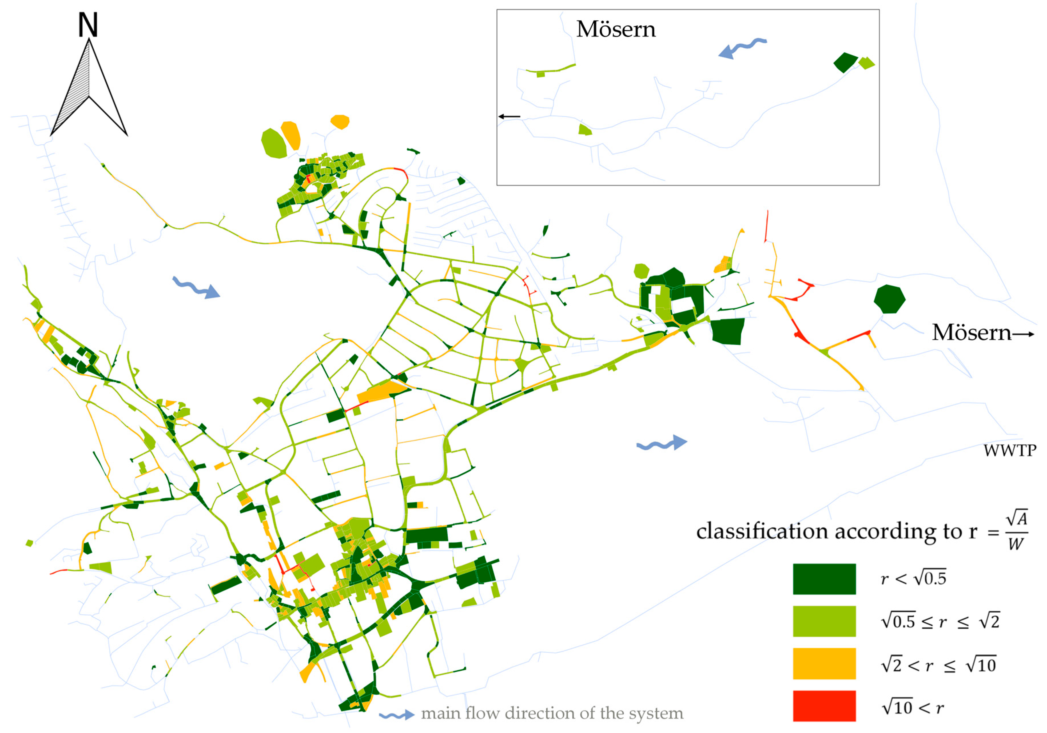
Telfs has one remote parcel, called Mösern. This part is about 3 km away and connected in the east of the system. For a better depiction, Mösern is shown in a separate image section in all figures of this paper showing the drainage system.

During a previous measurement campaign in 2014, three rain gauges were installed spatially distributed all over the area of Telfs. Their recordings are now used for this study as model input data. A model has been established and calibrated on measured water levels using the genetic calibration tool of PCSWMM [25]. It has then been tested for plausibility by comparing its simulated discharged volumes to the wastewater treatment plant to measurement data of the plant, further by comparing the simulated to the measured total pumping durations, and also through considering the operator’s assessment of the system’s behavior. An area of approximately 73 ha in total is connected to the sewer system in the model, with an average imperviousness of 58% [22]. This model is used as a reference system.

The only wastewater treatment plant (WWTP) is located southeast of the town. This plant treats the wastewater of five nearby communities (including Telfs) and its capacity is designed for 40,000 population equivalents. Accordingly, the drainage network of Telfs has to cope with draining also the wastewater of the other association members to the WWTP.

Historically the drainage system is a combined system, which was adapted over time by disconnecting several settlements (i.e., subcatchments) for alternative drainage options. Such options include e.g., the direct discharge of stormwater into the river Inn and decentralized methods such as local infiltration. This study focuses on sensor placement for calibrating the combined system. Only noticeably complex parts of the separate system are considered additionally. System parts are considered as noticeably complex when in order to model their hydraulic behavior anything other than conduits and junctions are necessary in the hydrodynamic model (e.g., storages or weirs).

A more detailed description of the model is provided by Tscheikner-Gratl et al. [10].

2.2. Implementation and Automation

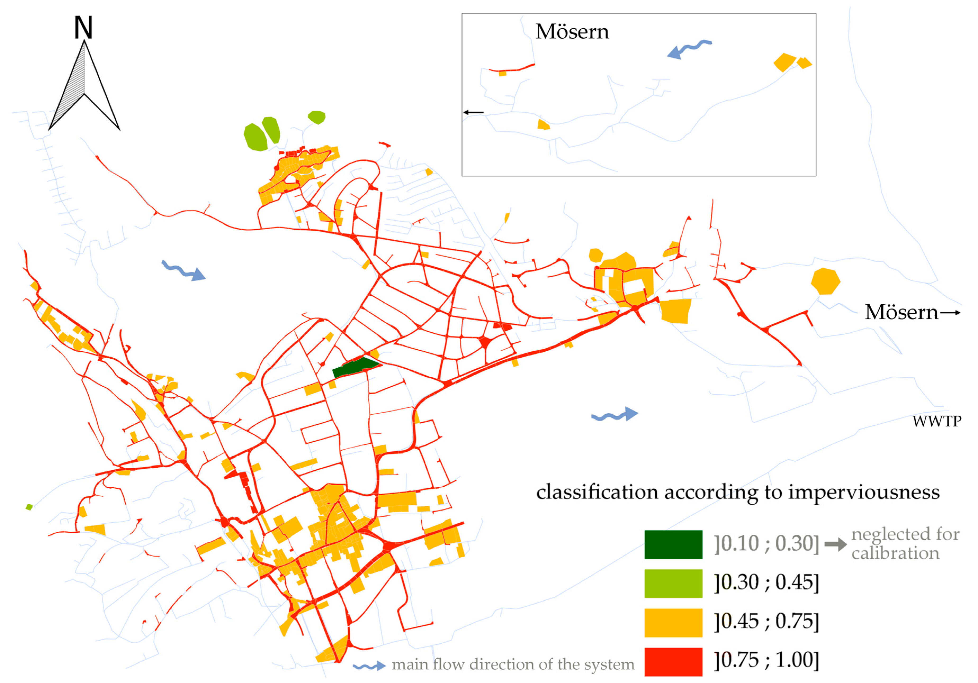
For modeling and hydrodynamic simulation, the software SWMM [26,27] is used. The investigations of this study are based on the variation of calibration parameters controlling the subcatchment’s runoff concentrations and their imperviousness. In SWMM, these attributes are expressed for each subcatchment by a value for the subcatchment width and the imperviousness, respectively. SWMM represents the subcatchments in a rectangular shape and therefore the width influences the flow time on the surface and in consequence the shape of the hydrograph on each subcatchment. In this work, we clustered subcatchments to assign them to the same calibration parameter. This reduces the total amount of calibration parameters significantly. Subcatchments are clustered according to their deviation from a quadratic shape taken from GIS data (a ratio between the coextensive square side length and the width, see Figure 1) and their land-use (imperviousness, see Figure 2) in the uncalibrated model.

The initial values of all subcatchments with the same color are further multiplied with the same respective parameter. We used four factors (parameters) for the width and three factors for the imperviousness. The group with the lowest imperviousness consists of only one subcatchment and is therefore assumed to have a neglectable impact on calibration. A change in one parameter consequently has an impact on variously spread subcatchments simultaneously.

Calibration parameter assignment as well as the subsequently performed calibrations and sensitivity analyses were automated by using the programming language R [28].

To calibrate the model and find a suitable set of parameters, an optimization algorithm based on a Nelder-Mead simplex [29] is used with the objective function of maximizing the Nash-Sutcliffe Efficiency in the regarded calibration point. This optimization algorithm is a derivative free numerical method for nonlinear optimization problems. This algorithm is applicable for the heuristic approach used here, as the calculation of derivatives for this multidimensional problem requires unreasonably large computational efforts and an analytical solution is unavailable.

2.3. Approaches to Assess the Suitability of Pipes as Measurement Sites

The identification of suitable locations to conduct measurements can be performed in various ways. This paper presents two main approaches to identify such suitable locations for measurements:

• Calibration to specific measurement layouts: At first, a calibration for each possible measurement site is executed separately. In a next step, combinations of different measurement locations based on the established results are tested for calibration.
• Sensitivity analyses: Local sensitivity analyses are carried out to assess which pipes are most sensitive to changes in the input parameter.

These two approaches are explained in more detail in the following subsections. They both rely on the same previously described parameter assignment as well as a precedent selection process for possible measurement sites. This selection is a decision process based on changes in the total inflow to the sewer network in order to restrict the possible measurement sites.

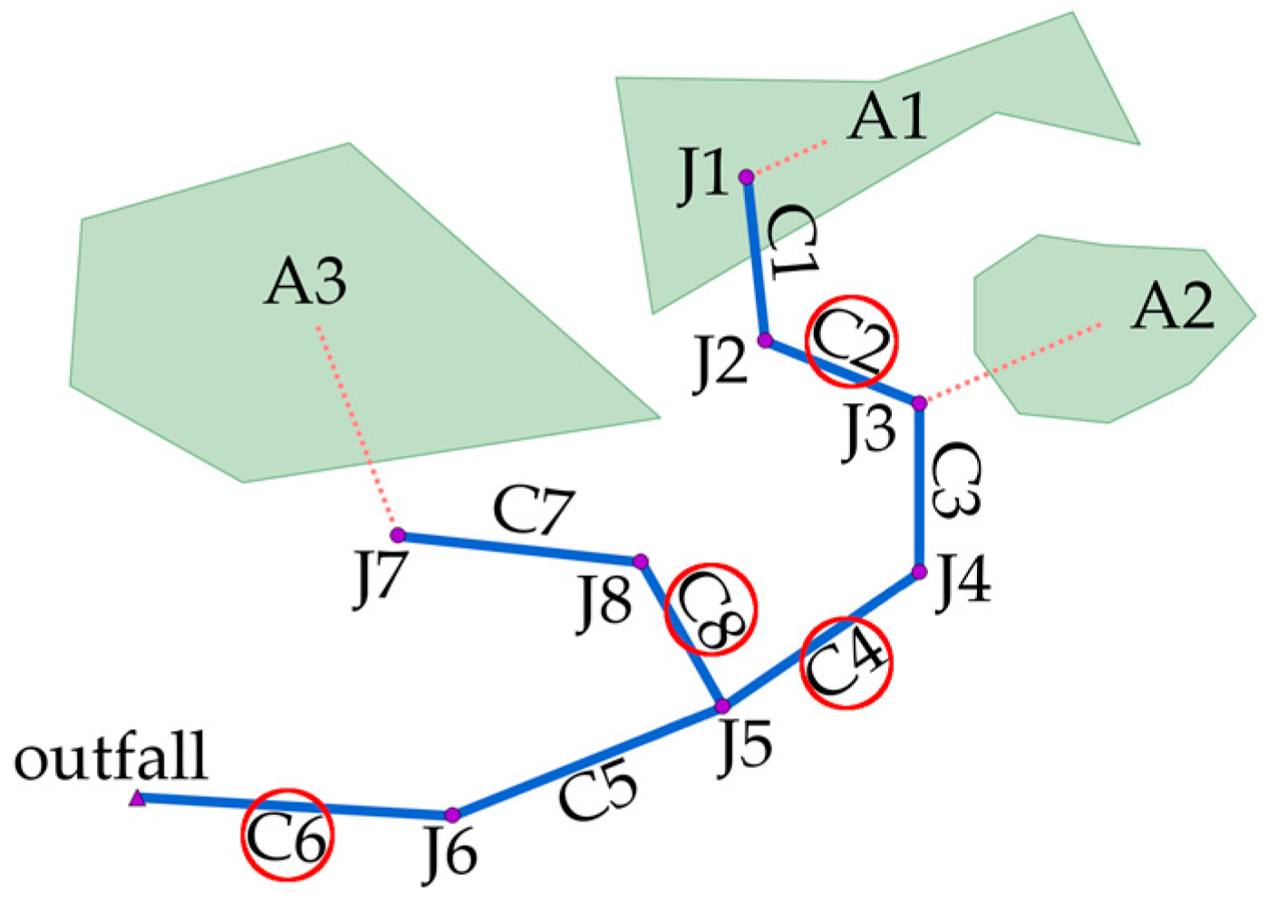
Although the total catchment area is relatively small, the model consists of over 3000 pipes and all pipes can theoretically be used individually as a measurement site. A first restriction in the choice of potential measurement locations is set in order not to test every single pipe section of the model as a calibration point, and thereby lower the necessary computational effort. The decision, if a pipe is considered to be a potential measurement location or not, is based on changes in the total inflow. A pipe is specified as a potential measurement location, if a subsequent change in the total inflow occurs. This is exemplarily depicted by means of the encircled conduits in Figure 3:

• before a junction, which is determined as an inflow node of a subcatchment
• before a junction, which has more than one incoming or outgoing connected conduits
• in conduits leading to an outfall

This classification leads to a reduction from over 3000 available pipes to 1094 potential measurement locations. Still, this amount would demand unreasonably large computational efforts for a mathematical solution of optimum measurement site selection, as it is used in Clemens [21] with 295 potential measurement locations. Only the simulation results of these 1094 pipes are then compared to their reference values. This comparison is mainly based on the evaluation of the Nash-Sutcliffe-Efficiency (NSE) [30] of the water level time series in each pipe. Additionally, other performance indicators are evaluated in order to increase the significance of the results. These include the Index of Agreement (d) [31], the correlation coefficient (r), the root mean square error (rmse) as well as the sum of the squared residuals (ssq). Differences of these values as well as their advantages and disadvantages for calibration can be found in Krause et al. [8].

In order to verify the model behavior and the algorithm for automatic calibration, the procedure of calibration with one calibration point each and the sensitivity analyses are executed with two different rainfall inputs. At first, a consolidated rain series [32] consisting of three real measured rain events, with peaks of 5.4, 9.2 and 4.8 mm/5 min respectively, taken from the existing rain gauges is applied. Then, the procedures are repeated for a design storm event type Euler II with a return period of 5 years, prepared according to Austrian design guidelines [33] with a peak of 12.2 mm/5 min.

2.3.1. Calibration to Specific Measurement Layouts

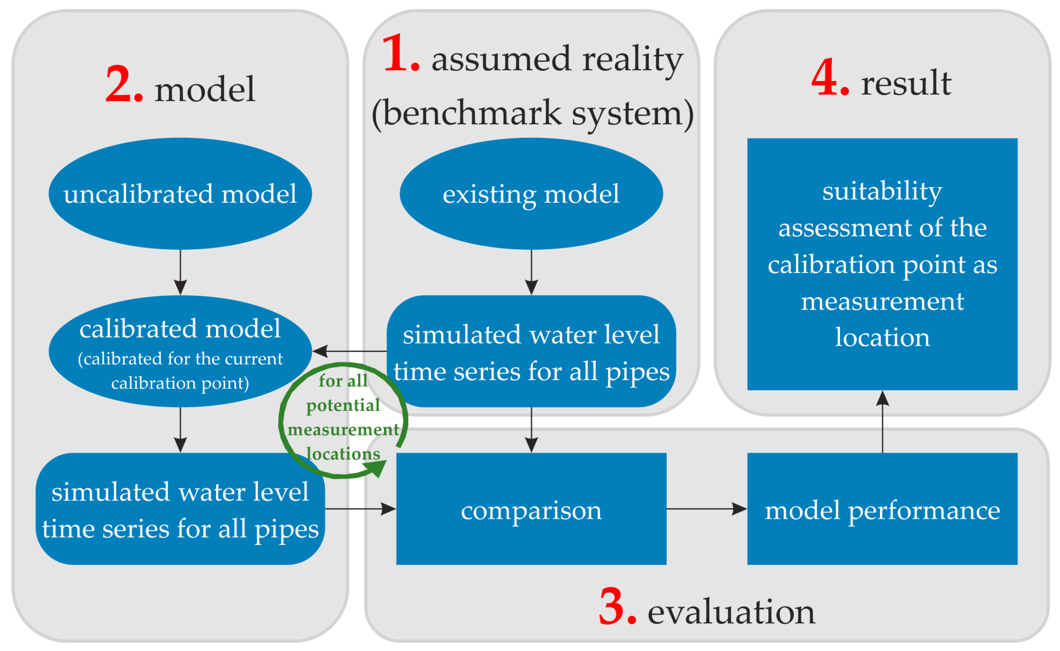
As a first approach, all of the 1094 remaining potential measurement locations are used to simulate separate calibration scenarios. In each scenario, only the dataset from one measurement site is used for calibration. Figure 4 shows the general scheme of this approach, as well as the way of abstracting the reality to the used benchmark system.

The method works as follows (enumerations corresponding to the numbering in Figure 4):

• The basis is an existing and for plausibility tested hydrodynamic model of the case study’s urban drainage network. Its simulation results are assumed to represent the reality i.e., to be measurement data of the system behavior. It serves as a reference system for all further investigations and benchmarks in this study.
• A new uncalibrated model is created from the existing reference model. This model is created by setting model parameters to typical values based on the analysis of available orthophotos while applying the same clustering as described in Section 2.3. It is then used to test different scenarios of measurement layouts for calibration. For each scenario, a calibration is carried out using the reference model as measurement. Each scenario results therefore in a newly calibrated model.
• Simulated water level time series from the newly calibrated models for each scenario are compared to their (assumed) measurements in the benchmark system. In order to ensure a multi-perspective view on the calibration results [9], different objective functions (NSE, d, r, rmse, ssq) are evaluated to compare the simulated with the reference water level time series and thus assess each calibration performance.
• This approach results in assessing the calibration performance of each calibration point based on the comparisons between model results and assumed system behavior (which are the reference model’s simulation results) in all pipes.

As a criterion for sufficient calibration, a threshold for the NSE at the respective measurement station of 0.9 is chosen (1.0 would represent a perfect fit). In a first run, over 1000 model calibrations are proceeded with one calibration point each. Then, the model performance of each calibrated model is evaluated.

The NSE values of all pipes in the network are evaluated statistically for each calibration scenario to assess the individual suitability of a pipe as a measurement station. These evaluations contain eleven values, i.e., the 10%, the 25%, the 50% (median), the 75% and the 90%-quantile and minimum, maximum and mean values of the NSEs as well as the standard deviation over the network. Furthermore, the mean absolute change in the NSEs and the number of pipes with a NSE > 0.9 are calculated. The median, the mean absolute change and the number of pipes with a NSE > 0.9 are regarded as the most meaningful values. These values are used for the assignment of an individual prospect of success for an accurate calibration to each measurement station.

To combine the advantages of different measurement sites, calibration to combined measurement stations is additionally performed by using the results of the first calibration procedure to single pipe measurements. Combinations of different calibration points are assumed as a measurement campaign and calibration is proceeded until the NSE exceeds a value of 0.9 in all of these pipes.

With 1094 individual potential measurement locations, a total number of ${\sum }_{k=2}^{1094}\frac{1094!}{\left(1094-k\right)!}=3.12\ast {10}^{2850}$ combinations are possible. As this represents an unrealistic computational effort, a second restriction in the selection of potential measurement campaigns is made in order to keep the computational effort within reasonable limits. Only systematically sampled measurement combinations are tested for calibration. The combinations are identified according to the following procedure:

• A first pipe a is chosen as a measurement point from the foregoing ranking of calibration to single pipes. Therefore, calibration points with a resulting high calibration performance are taken into consideration.
• A second pipe b is selected to enhance the model’s agreement to the reference model after it was calibrated to pipe a. For this, attention is paid to pipes showing a poor fit after the calibration to pipe a. Out of the foregoing calibrations to single pipes, a scenario is looked up that results in a good fit for exactly those pipes. The underlying calibration point of this detected scenario is then selected to be pipe b, the second measurement station.
• An automated calibration to those two measurements is executed. The same threshold of NSE > 0.9 has to be fulfilled for both hydrographs.
• A third suitable pipe c for an additional measurement is determined by regarding the NSE values calculated after the calibration for pipes a and b together. The selection of pipe c now follows the same rules as the selection of pipe b.
• Again, a calibration for pipes a, b and c is performed, until all of the three reach a NSE of at least 0.9.
• This scheme can be applied repeatedly to add more calibration points. The stop criterion is the number of measurement sites planned. In this work, we sampled from two up to a maximum of six pipes, which represents the financial constraint in the number of measurement sites.

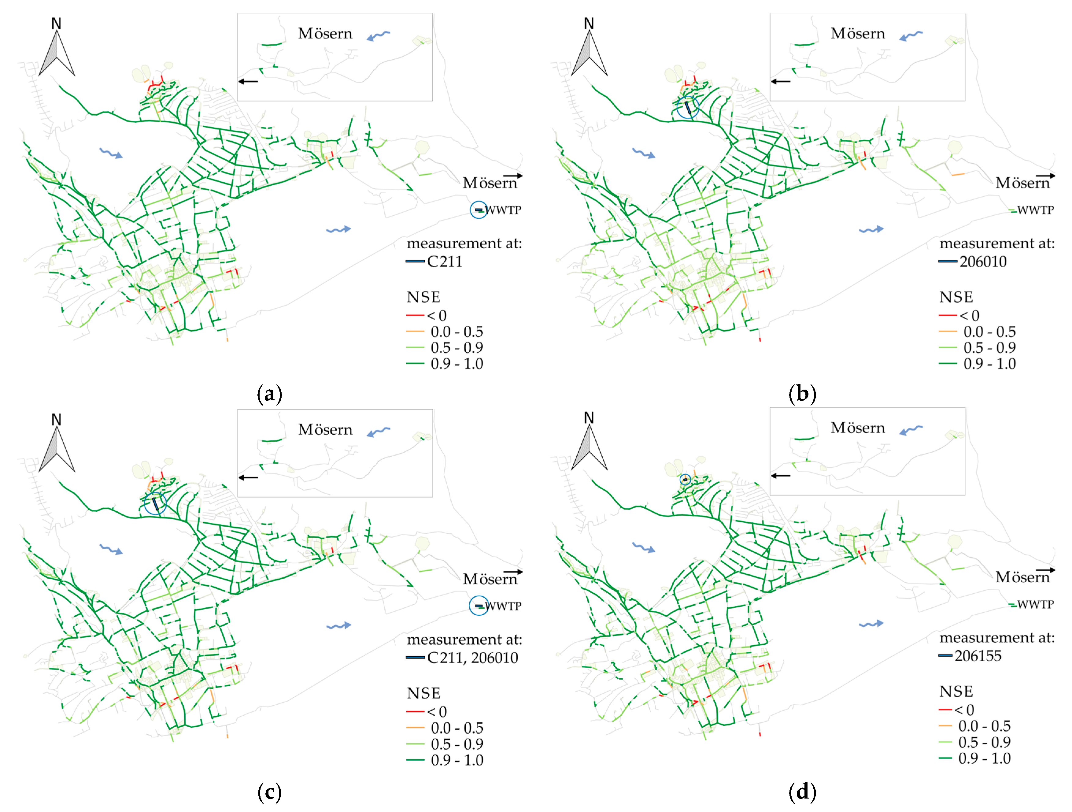
Figure 5 exemplifies the procedure explained above.

Step 1 (Figure 5a): As a first measurement point the pipe C211 (encircled) is chosen, due to a good fit to the overall network. This calibration result is highly rated, because 824 out of 1094 pipes result in a NSE > 0.9 with a median value of 0.944. However good the fit, there are still negative NSEs occurring in the northern part of the network.

Step 2 (Figure 5b): The choice of an additional measurement site is thus focused on a resulting good fit in those parts, regardless of the fit in the rest of the model. There, the best agreement can be reached by calibrating for pipe 206010.

Step 3 (Figure 5c): A new calibration for C211 as well as for 206010 is performed and results in NSEs shown in Figure 5c. Again, system parts with non-sufficient agreements are identified in the northern part.

Step 4 (Figure 5d): An additional measurement station 206155 (with original results according to Figure 5d) is determined in order to improve those links in particular.

Step 5: A calibration for C211, 206010 and 206155 is conducted and the resulting NSEs are evaluated.

Step 6: Another pipe can be chosen and added to the measurement campaign to improve specific system parts with occurring low NSEs. This procedure is continuously repeated until the wanted number of measurement sites is reached.

2.3.2. Sensitivity Analyses

Independent of the straight-forward calibrations described above, sensitivity analyses to the same calibration parameters as in the previous approach are performed [34]. Therefore, 1000 models are created and simulated with random parameter sets complying with set boundary conditions. Then, the simulation results of the randomly created models are compared to the results of the reference model. For this comparison, each pipe is regarded individually, unrelated to the behavior of other pipes. The idea behind is the assumption that pipes that clearly respond to changes in the input parameters are good measurement locations to determine those parameters. Pipes with nearly steady values do not respond to changes in the model parameters and are not suitable for calibration. So the amount of information in a measurement is assumed to increase with the sensitivity of the pipe [35].

3. Results and Discussion

The following results are based on the evaluation of over 20,000 simulation runs. Each previously described approach will be discussed separately with its respective results. Further comparisons and integrated considerations are also given at the end of this chapter.

3.1. Calibration to Specific Measurement Layouts

To compare the results of calibrations with scenarios of varying measurement data samples (single as well as combined calibration points), different common statistical values for the NSEs in all pipes after calibration are evaluated to assess the calibration performance.

This computational run was the most CPU-intensive as over 7500 simulations were executed during the optimization procedures. Even though, for the 1094 calibration scenarios to single pipe measurements with the measured rainfall, only 299 succeeded in a NSE > 0.9 at the regarded calibration point. For the calibration scenarios with the design storm, only 206 out of 1094 calibrations were successful.

Figure 6 shows the network with each pipe colored according to the calibration performance after the model has been successfully calibrated to this pipe, using the measured rain events as input. To represent the calibration performance, the number of pipes that exceed a NSE of 0.9 after model calibration is the chosen statistic presented in Figure 6.

Figure 6 also shows where calibration is not necessary or not possible. The uncalibrated model has been a rough estimation of the model parameters. It already showed up a good agreement (NSE > 0.9) for those pipes depicted as “cal. not necessary”. Therefore, calibrations with the aim of improving the agreement in those pipes are not necessary. Further pipes are depicted as “cal. not poss.”, which means that a calibration to these pipes was not possible. In the cases of considering these pipes as calibration points, the optimization algorithm could not succeed in reaching the determined threshold and thus could not meet the calibration criteria.

For a better understanding of Figure 6, two points of the network are discussed exemplarily in the following. The two outlets to the wastewater treatment plant are colored in light green and blue, respectively. Considering the northern (light green) pipe as a single measurement station, between 718 and 876 pipes result in a NSE > 0.9 when comparing the calibrated model to the reference model. The other (blue) outlet has not been considered as a calibration point, because this pipe already exceeded the threshold of NSE = 0.9 when comparing the uncalibrated model to the reference model. Consequently, an optimization aiming at maximizing the NSE at this point is not necessary.

Figure 6 does not allow drawing significant conclusions about the general location of such sites. A slight tendency can be made out for efficient calibration points to be located downstream. Nevertheless, high performances are also indicated occasionally with calibration points at upstream ends of pipe branches.

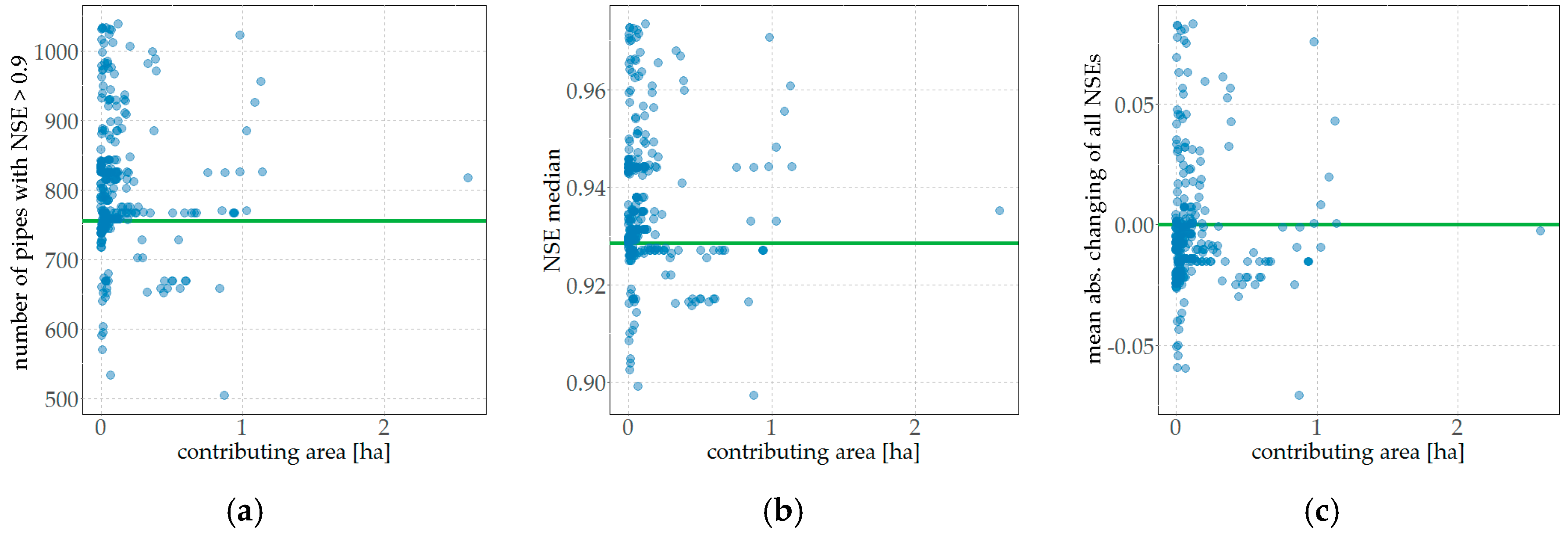
In Figure 7a, the number of pipes with a NSE > 0.9 is plotted. Figure 7b shows the median of all evaluated NSE values after a calibration, depending on the connected impervious area to the applied calibration point. In Figure 7c, the averaged absolute change in the evaluated NSE compared to the uncalibrated model is shown.

Also other evaluations of relationships in the calibration performance, e.g., dependencies on the diameter or the stream hierarchy of the measured pipe (the calibration point) etc., show similar scattered values.

The calibration approach is continued with the sampling of different pipes to a measurement campaign. The presented results of the calibrations using multiple calibration points simultaneously are restricted to the results of one of the established combinations. This measurement campaign consists of five calibration points and resulted in the best model performance compared to the other investigated combinations (11 in total). The resulting NSEs in all pipes are shown in Figure 8.

1025 out of 1094 evaluated links (93.7%) result in a NSE > 0.9 with a median value of 0.97. Only six pipes result in a NSE < 0, indicating that the mean value of their simulated water level time series would provide a higher NSE than the predicted values. These numbers represent a nearly perfect agreement of the model to the reference model after calibration. Therefore, this measurement campaign is highly rated to apply the here used calibration procedure to.

3.2. Sensitivity Analyses

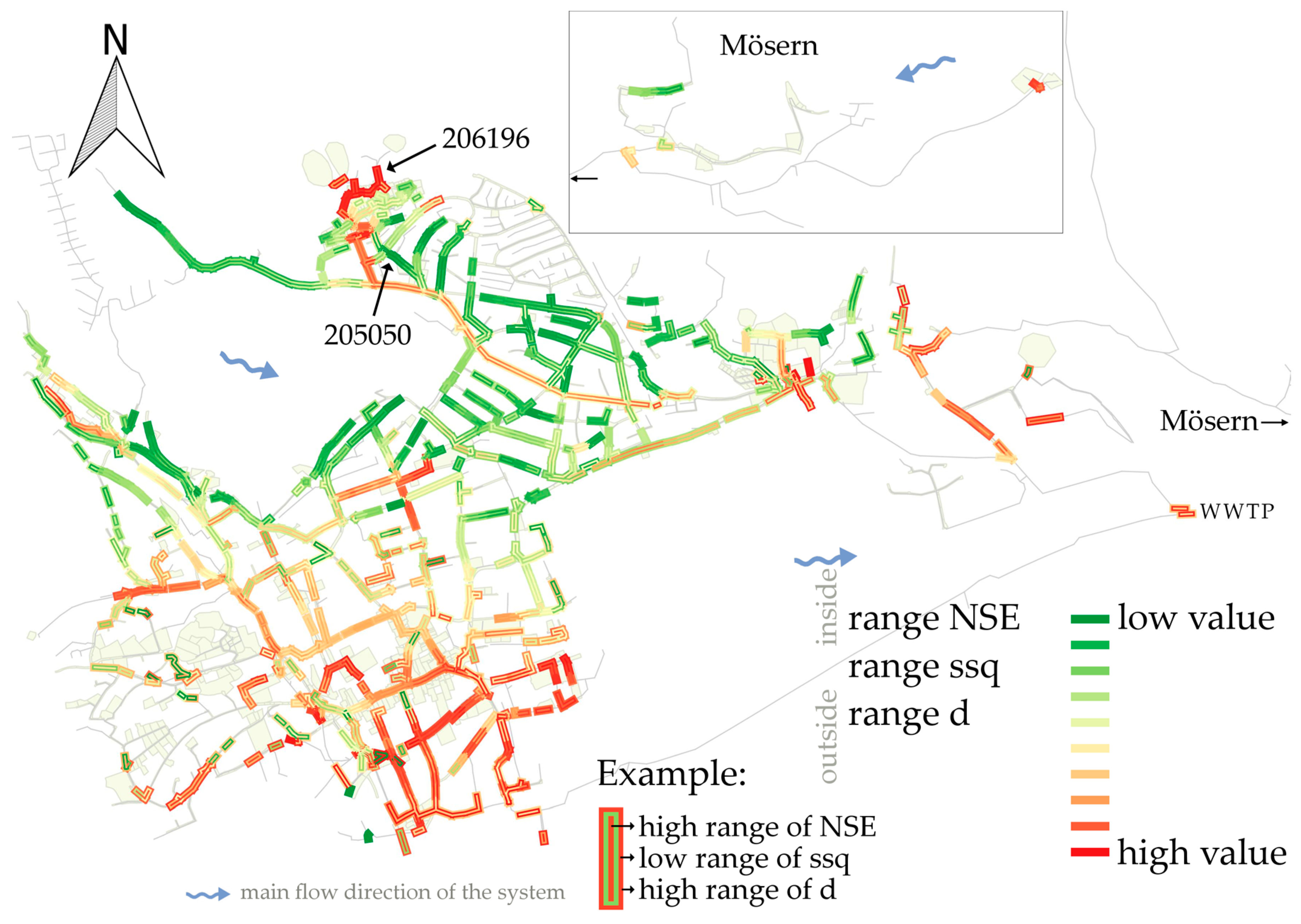
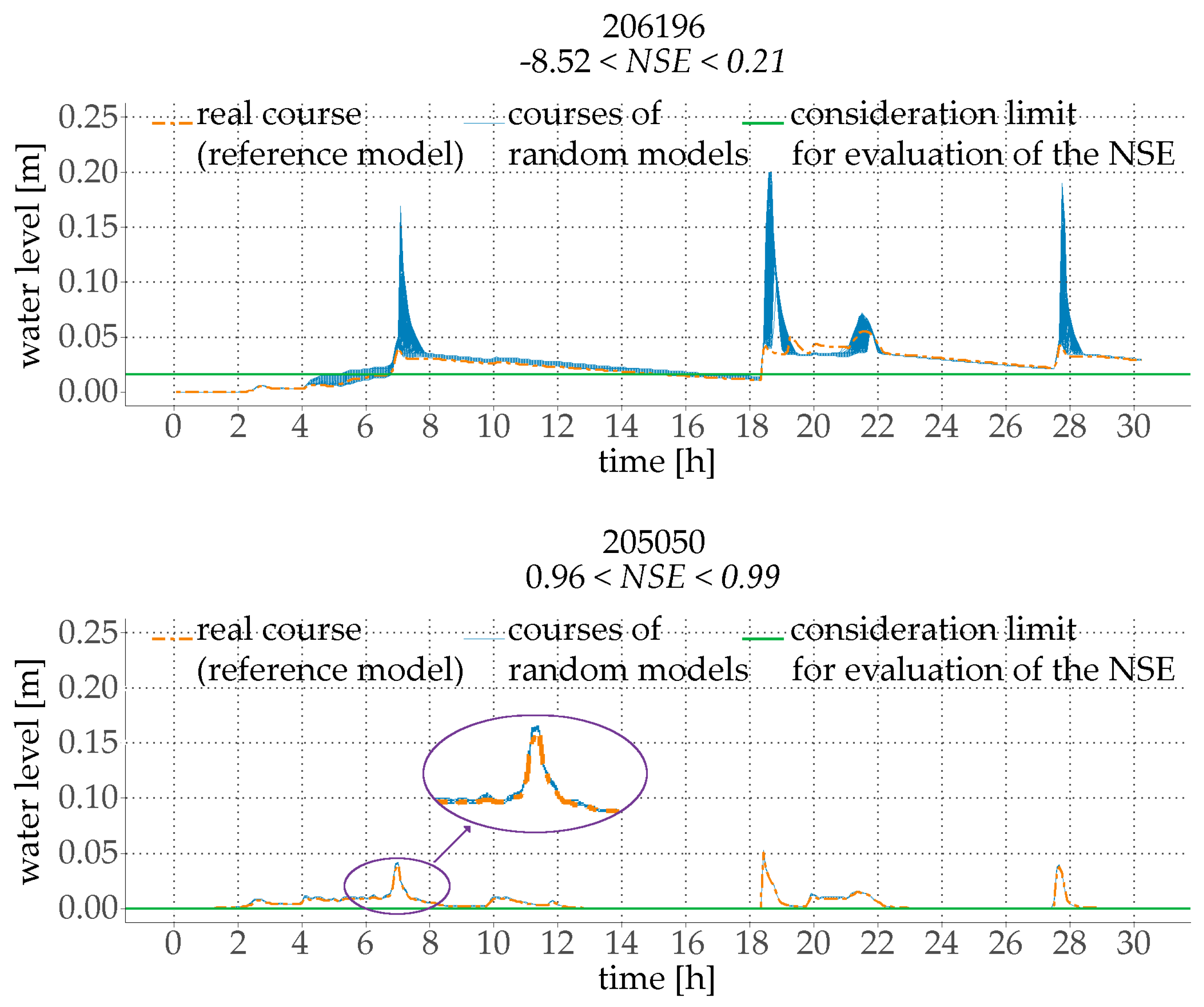
The sensitivity analyses provide recognizable tendencies, where data collection for calibration appears to be efficient. Figure 9 shows the network with each pipe colored according to the resulting ranges of five different performance indicators. The innermost color represents the range of the NSE, the outermost stands for the range of d. The closer to the red end of the spectrum that a pipe is colored, the more sensitive it is to changes in the calibration parameters. Pipes directly connected to high inflow rates (e.g., from large subcatchments) and pipes lying more downstream and/or connected to outfalls show high sensitivities to random parameter changes. Therefore, they are considered as recommended measurement locations. Their sensitivities indicate a high calibration performance and model performance if they are used as calibration points. The two pipes with the highest (206196) and lowest (205050) occurring range are highlighted in Figure 9.

For a more detailed depiction, Figure 10 shows the resulting water level time series of the reference model compared to the variations of the random models for these pipes. Periods with dry weather flow (values below the horizontal mark) are neglected when calculating the NSE (and all other objective functions) in order to prevent biased results caused by a good data fitting during quasi-static low flow periods.

The highest range of the NSE due to a random parameter variation occurs in pipe 206196 (Figure 10, upper graph). The accordance between random models and the reference model ranges from values of −8.52 to 0.21. Conversely, pipe 205050 (Figure 10, lower graph) shows the lowest sensitivity to parameter changes. Thus, the resulting flow depth course in pipe 205050 is rather independent of the calibration parameters whereas results for pipe 206196 strongly depend on the parameter choice. Both pipes are located upstream at the very beginning of a branch. Pipe 206196 drains a large subcatchment with higher inflow rates while only a small area is connected to pipe 205050.

3.3. Final Recommendations for Measurement Sites

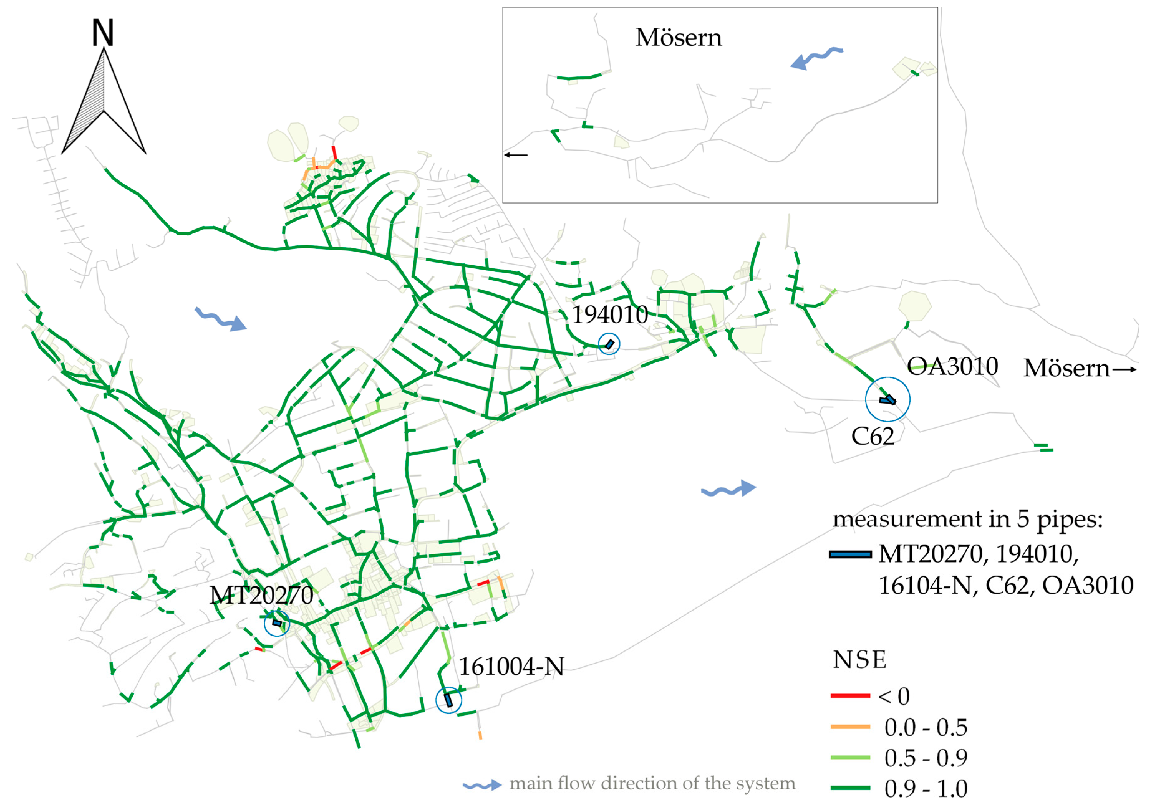
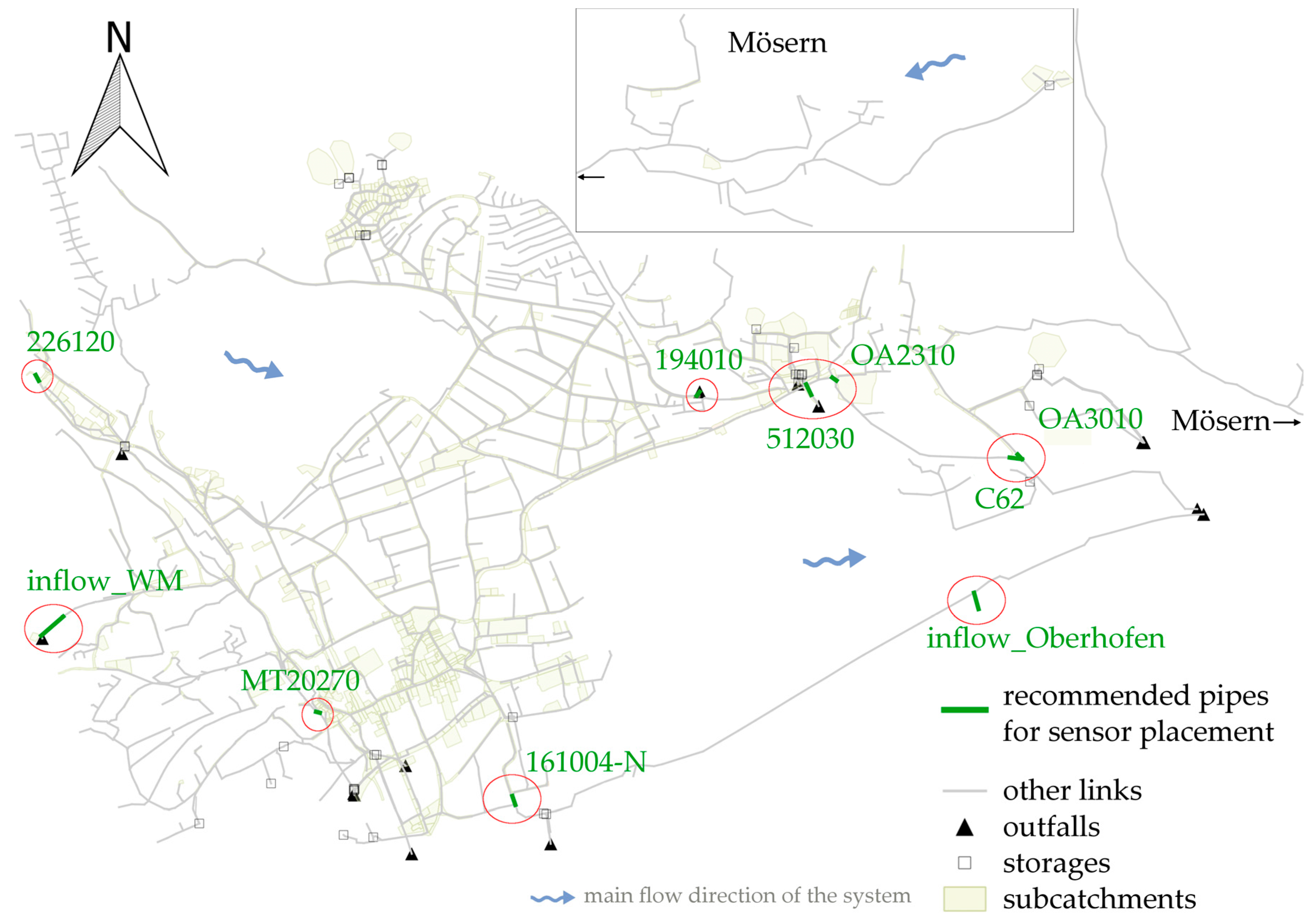
Finally, several efficient calibration points are identified for this specific case study. The final recommendations are shown in Figure 11, where the results from the different approaches (calibrations and sensitivity analyses) are combined.

They are mainly located at the end of collector branches of the combined sewer system (MT20270, 161004-N, OA3010, C62, OA2310). In separated drainage networks, larger subcatchments should be monitored at locations prior to outlets discharging into receiving water bodies (512030, 194010). However, it is considered to be important not only to measure right before outlets, but also that calibration data should be collected in collector pipes spread over the entire network. This allows the identification of significant model parameters in terms of influential subcatchments on a more detailed level [36].

Apart from the results of the previously explained approaches, external inflows should be quantified for additional reasons of economy. This includes known discharges from industrial companies (226120) as well as inflows from external catchments, i.e., adjacent municipalities (here inflow_WM, inflow_Oberhofen) into the network. As the wastewater treatment plant is operated jointly, related expenses can be allocated to each of the municipalities depending on those measurements.

Additionally, the case study’s operator roughly estimated favorable locations of measurement sites based on his empirical knowledge of the drainage network. There is a good agreement between the pipes theoretically recommended as measurement sites by means of the method described above and those suggested by the operator. This agreement confirms the plausibility of the approach. However, additional suggestions for measurements are locations with known operational problems (e.g., capacity overload).

All of the approaches use seven subcatchment-related parameters for calibration. This reduces the degrees of freedom of the automatic calibration algorithm to a reasonable extent. Consequently, the change of one parameter affects various subcatchments all over the catchment simultaneously and a differentiation between subcatchments lying upstream and downstream to the measurement site lapses. The results show a certain independence of the consequences of parameter changes from the actual location of the measurement. Thus, no correlation between characteristics of the measurement site (e.g., location, diameter, flow, etc.) and calibration performance could be found.

Furthermore, although the used numerical optimization algorithm for calibration may find suitable solutions efficiently, it is likely to converge at a local optimum and to miss the global optimum. As such, it is advisable to perform the calibration with different initial conditions.

However, the performed sensitivity analyses allow the derivation of systematic trends. High sensitivities can be seen in collector sewers and pipes with high inflow rates, meaning that those pipes are good locations for calibration. This observation corresponds to the advices for sensor placement on a network scale given in Skjetne et al. [17].

4. Conclusions and Outlook

This paper presents a heuristic approach for an experimental design of measurement campaigns and allows the identification of measurement sites for an efficient model calibration. The testing of different measurement layouts, the evaluation of the calibration performance as well as the impacts of parameter variations on the water level time series in every pipe is enabled by a model-based methodology. This makes it especially useful for setting up a completely new measurement campaign with no or few existing previous measurement data.

Even though this case study is a small catchment, its model contains over 3000 pipes and computational effort had to be kept manageable by setting some restrictions. Firstly, focus was led on the decisive network parts, i.e., by neglecting most of the independent sewer branches without a connection to the WWTP (stormwater sewers). Secondly, the here used calibration algorithm was implemented with seven calibration parameters for the whole model, of which all are adapting subcatchment-related characteristics of multiple subcatchments simultaneously. Thirdly, neither every single pipe nor every possible combination of pipes was tested as a calibration scenario. Only systematically determined calibration points and combinations are considered in the evaluations.

Regarding the presented heuristic approach, it may not be able to show up the optimal solutions for measurement campaigns. Nevertheless, it is sufficient to compare different possible measurement sites for calibration. This further allows finding a suitable solution for the question of measurement site selection in a relatively short time frame and with an appropriate computational effort.

As a result, a number of 10 pipe sections are provided for recommendable measurement sites. They do not only meet the criteria of efficiency for calibration (i.e., the six measurement sites established with the here presented methodology), but also cover operational and economic aspects (four more measurements). Thus, this study emphasizes a calibration to strategically distributed measurements within the network topology in contrast to favor data collection in pipes where operational problems occur. The results indicate an increased model performance when calibration data is available for collector sewers and sewers placed immediately after inlets with high inflow rates. This exemplifies the crucial role of high inflow rates to hydrodynamic model predictions (e.g., flooding incident, combined sewer overflow).

As an outlook, further studies could enhance the methodology by increasing the number of calibration parameters by considering the subcatchment’s location within the network (e.g., upstream or downstream of the regarded calibration point) or the inclusion of redundant measurements in order to cope with possible failures of sensors or errors in the measurements.