Article

Using a Distributed Hydrologic Model to Improve the Green Infrastructure Parameterization Used in a Lumped Model

1
ReNUWIt Engineering Research Center, Colorado School of Mines, 1500 Illinois St., Golden, CO 80401, USA
2
Hydrologic Science and Engineering Program, Department of Geology and Geological Engineering, Colorado School of Mines, 1500 Illinois St., Golden, CO 80401, USA
*
Author to whom correspondence should be addressed.
Current address: Enginuity Engineering Solutions, 10106 W. San Juan Way, Suite 215, Littleton, CO 80127, USA.
Water 2018, 10(12), 1756; https://doi.org/10.3390/w10121756
Submission received: 12 October 2018 / Revised: 20 November 2018 / Accepted: 25 November 2018 / Published: 29 November 2018

Abstract

:
Stormwater represents a complex and dynamic component of the urban water cycle. Hydrologic models have been used to study pre- and post-development hydrology, including green infrastructure. However, many of these models are applied in urban environments with very little formal verification and/or benchmarking. Here we present the results of an intercomparison study between a distributed model (Gridded Surface Subsurface Hydrologic Analysis, GSSHA) and a lumped parameter model (the US Environmental Protection Agency (EPA) Storm Water Management Model, EPA-SWMM) for an urban system. The distributed model scales to higher resolutions, allows for rainfall to be spatially and temporally variable, and solves the shallow water equations. The lumped model uses a non-linear reservoir method to determine runoff rates and volumes. Each model accounts for infiltration, initial abstraction losses, but solves the watershed flow equations in a different way. We use an urban case study with representation of green infrastructure to test the behavior of both models. Results from this case study show that when calibrated, the lumped model is able to represent green infrastructure for small storm events at lower implementation levels. However, as both storm intensity and amount of green infrastructure implementation increase, the lumped model diverges from the distributed model, overpredicting the benefits of green infrastructure on the system. We performed benchmark test cases to evaluate and understand key processes within each model. The results show similarities between the models for the standard cases for simple infiltration. However, as the domain increased in complexity the lumped model diverged from the distributed model. This indicates differences in how the models represent the physical processes and numerical solution approaches used between each. When the distributed model results were used to modify the representation of impermeable surface connections within the lumped model, the results were improved. These results demonstrate how complex, distributed models can be used to improve the formulation of lumped models.

1. Introduction

Stormwater management is increasingly becoming integrated and interdisciplinary, and there are a growing number of hydrologic models being used to address the challenges of urban hydrology [1,2,3]. Many of these models can simulate integrated surface and subsurface flow with the aim of representing the relevant physical processes that influence the hydrologic response at varying scales [4,5]. Distributed models more accurately represent the built environment at varying scales, can integrate local geographic information, and have fewer lumped parameters that need calibration [6,7,8]. However, they also require larger amounts of input data and require substantially more computing resources [7]. Lumped models require less input data, and less computational time, and when calibrated have many advantages over distributed models [9]. However, representing the urban system requires many different parameters with varying spatial patterns that present challenges to lumped models that use uniformly distributed parameters [5,10]. With multiple models to choose from, decision makers are left with the challenge of determining which modelling approach is most appropriate for urban systems. Is there a way that distributed models can inform parameterization in lumped models? Thus, providing decision makers with the appropriate tools and information needed to assess difficult urban stormwater challenges.
A challenge when evaluating model capabilities and accuracy is the lack of published analytical solutions [11] and known coupled surface-subsurface analytical solutions. There are two options to evaluate model performance:
  • Compare solutions to observations.
  • Compare simulations using benchmark cases and compare results to other published solutions [4,12,13,14,15,16,17].
The challenge with the first option is that lumped models are typically calibrated to observations, making exposure of their internal states challenging. Previous studies found that lumped model results vary significantly with small changes in lumped parameters, such as percent impervious, that vary in complexity based on the model resolution and spatial patterns [5,18,19,20,21]. In addition, previous studies also identify the need to reduce model uncertainty [22]. Even though models are calibrated to observations, it is not clear how transferrable these parameters and approaches are to nonstationary future conditions [4,9]. The second option requires accepted and established standard procedures and benchmark test cases.
There have been several successful intercomparison exercises in the field of hydrology, such as the Project for Intercomparison of Land-Surface Parameterization Schemes (PILPS) [23,24,25,26,27,28], the Distributed Model Intercomparison Project (DMIP) [29,30], and Intercomparison for Integrated Hydrologic Models (IH-MIP) [4,17]. These studies have compared lumped and distributed models extensively, evaluating model performance and capabilities at varying scales, but few studies if any have considered the urban system that includes green infrastructure when intercomparing hydrologic models. In addition, a goal of some of the intercomparison exercises has been to try to determine global parameters for different schemes based on validated results [23,24,25,26,27,28,29,30]. The PILPS studies indicate that global catchment parameters could be used by modelers using different land-surface schemes [27]; our study expands upon this previous work.
In this paper, we present the results of an intercomparison performed for distributed and lumped hydrologic models in a completely urban domain that includes green infrastructure. It tests and compares the distributed and lumped models, uses the distributed model to inform the lumped model, and improves the lumped model’s representation of green infrastructure. We accomplish this by performing a new urban case study that compares and evaluates each model’s representation of green infrastructure in a completely urban domain. We then compare basic model configurations using two of the idealized benchmark test cases presented in Maxwell et al. [4]. These test cases emphasize the role of various model components and their interactions. The benchmark cases compare the flow components of the distributed hydrologic model (Gridded Surface Subsurface Hydrologic Analysis, GSSHA), and one lumped model (the EPA Storm Water Management Model, EPA-SWMM). This study extends the work of Sulis et al. [15], and Maxwell et al. [4,17]. The guiding principle of this work is like the previous studies in which different integrated hydrologic models perform standardized benchmark problems to gain an increased understanding of the representation of coupled hydrologic processes and how they can be used to inform and improve modeling schemes and systems [4,17,27].
The intercomparison starts with the new urban case study between a fully coupled distributed model (GSSHA) and a lumped model (EPA-SWMM) within a real-world urban domain in Denver, CO, USA. This study evaluates each model’s capability to model green infrastructure within an existing urban watershed and the resulting impacts to water quantity. Since no known solution is available for this watershed and simulated implementation of green infrastructure, we compare and discuss the results. It should be noted that this work expands upon the work completed by Fry and Maxwell [7] that used regional calibration parameters for a distributed model in the Denver metro area. Next, we perform the simple benchmark cases for the models, to evaluate differences seen between the distributed and lumped models for the urban case study. Like the urban case study, no known solution is available for these simple benchmark cases, so we compare and discuss the results. Finally, we synthesize the results and present a methodology based on the work performed by Fry and Maxwell [7] that incorporates the distributed model results into the lumped model. The methodology informs lumped model parameters and improves performance and accuracy when compared to the distributed model. We discuss and compare the results to provide better understanding and confidence in the use of both distributed and lumped hydrologic models to represent green infrastructure in urban environments.

2. Materials and Methods

2.1. Description of Models

2.1.1. GSSHA

Gridded Surface Subsurface Hydrologic Analysis (GSSHA) is a physically-based, distributed-parameter, structured grid, hydrologic model that simulates the hydrologic response of a watershed subject to given hydro meteorological inputs. The GSSHA uses a uniform finite difference grid to divide the watershed. Processes that occur before, during, and after a rainfall event are calculated for each grid cell and then the responses from individual grid cells are integrated to produce the watershed response. The governing equations for GSSHA are:
Manning’s Equation (2-D):
Q = 1 n A R 2 3 S f 1 2
Diffusive Wave Equation (2-D):
S f = S 0 Δ d Δ x
where n is a roughness coefficient, A is the area (L2), R is the hydraulic radius (L), and Sf is the friction slope (L/L). S0 is the land surface slope (L/L) and d is the surface depth (L) [31].
GSSHA uses a two-step explicit finite volume scheme to route 2-D overland flow. GSSHA computes overland flows based on flow depths (heads) and updates volumes based on the computed flows. The algorithms used in GSSHA are simple when compared with more sophisticated implicit finite difference and finite element schemes. GSSHA calculates the friction slope between one grid cell and its neighbors as the difference in water surface elevations divided by the grid size. Unlike the kinematic wave approach, this diffusive wave approach allows GSSHA to route water through pits or depressions. GSSHA uses Manning’s Equation to relate flow depth to discharge [31]. Infiltration options in GSSHA include 1-D Richard’s Equation, Green and Ampt, multi-layer Green and Ampt, and Green and Ampt with Redistribution (GAR). For this analysis infiltration is simulated using the traditional Hortonian Green and Ampt methods, which are simplifications of the Richards Equation in 1-D [32,33,34].

2.1.2. EPA-SWMM

The EPA Storm Water Management Model (SWMM) is a dynamic rainfall-runoff simulation model that computes runoff quantity and quality from primarily urban areas. SWMM is a nonlinear reservoir runoff model based on the continuity equation and momentum equations.
Conservation of Mass:
d t = i e f q
Manning’s Equation:
Q = 1.49 n W S 1 2 ( d d s ) 5 3
where i is the rate of rainfall (L/T), e is evaporation rate (L/T), f is the infiltration rate (L/T), and q is the runoff rate (L/T). Manning’s equation is modified where W is the width through which runoff flows through the subcatchment area multiplied by the height (dds), and the hydraulic radius is related to the depth (dds) [35].
The runoff component of SWMM operates on a collection of subcatchment areas that receive precipitation and generate runoff. SWMM treats each subcatchment area as a non-linear reservoir. SWMM calculates surface runoff using a method of planes in which it applies a water balance equation over the subcatchment for each time step. The subcatchment is broken down into pervious and impervious planes, based on the parameters input. Each plane has inflows from precipitation, and upstream sub catchments, and outflows from infiltration, evaporation, and surface runoff. SWMM determines the reservoir capacity with the depression storage parameter. Overland flow occurs when runoff exceeds the depression storage, and SWMM calculates outflow using Manning’s Equation [35,36,37]. Infiltration options in SWMM include Horton’s Equation, SCS-CN, and Green and Ampt. To be consistent with GSSHA, we chose to use the Green and Ampt method for infiltration.

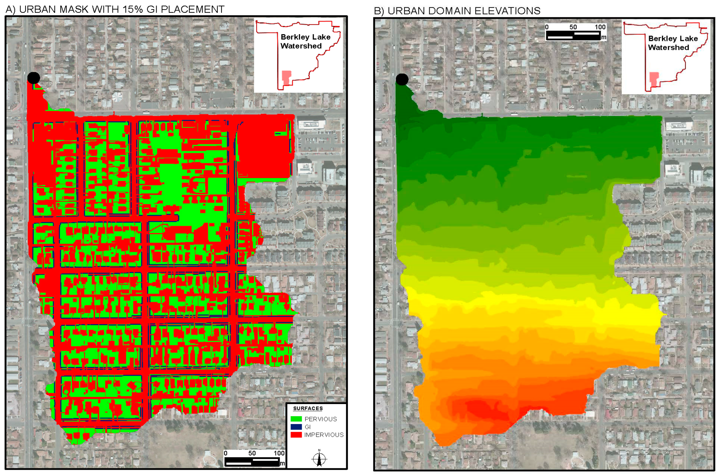
2.2. Urban Benchmark Case Study: Green Infrastructure

One of the challenges of modeling green infrastructure (GI) in urban environments is the heterogeneous arrangement of different land surfaces. Studies have shown that lumped parameter models may not account for the variabilities of the urban environment [5,18,19,20,38,39]. This case study builds upon a simulation test case presented in Fry and Maxwell [7] in which they evaluate the impacts of GI on water quantity within an urban watershed using regional calibration parameters in a distributed coupled model. This case study compares the use of a distributed coupled model (GSSHA) with a lumped model (EPA-SWMM) to evaluate the impacts of GI on total storm runoff (peak flow and volume), infiltration, and storage in an urban environment. The urban benchmark case study consists of a highly complex domain with varying parameters. The case study uses the same study site previously modeled, a neighborhood in the Berkley Lake watershed in Denver, Colorado. The size of the sub-watershed is 26.14 hectares. The model includes the built environment, which consists of a mix of residential, commercial and high density residential land uses. The urban case includes five different synthetic storm simulations representing higher frequency to lower frequency events (2, 5, 10, 50, and 100 Year). The analysis assumes each simulated event to be under dry antecedent moisture conditions based upon the soil type and as a single event. The urban case uses storm events based upon the Urban Drainage and Flood Control District’s criteria for rainfall in the Denver metro area [40]. The rainfall totals for each 2-h storm event were 2-Year: 27.92 mm, 5-Year: 39.38 mm, 10-Year: 45.55 mm, 50-Year: 66.07 mm, and 100-Year: 75.46 mm. The urban case incorporates green infrastructure within under-utilized pervious areas within the domain using the methodology described in Fry and Maxwell [7]. This method converts under-utilized pervious areas, such as tree lawns, medians, and existing green space, to GI at the following intervals 15%, 25%, 35%, and 50% of the area. Input parameters for the domain and GI are provided in Table 1, and visually shown in Figure 1.
We implemented GI in EPA-SWMM through the Low Impact Development (LID) controls module. The module allows the user to specify a type of GI, the size of the GI, the number of them within the basin, and the amount of impervious area routed to them [36]. The GI type chosen in SWMM was a bioretention cell, which allows the user to modify the storage and soil parameters. The size was based on a cell size of 1 m2 to be consistent with the distributed model. The number or amount of GI was based on the percent area converted to GI divided by 1 m2. And the amount of impervious area routed to each GI was determined via a spatial analysis, in which we evaluated the directly connected impervious areas routed to each bioretention cell.
We modeled green infrastructure in GSSHA using a high-resolution grid (1 m2). We assigned an elevation to each cell based on the digital terrain. The model incorporates land use features based on geographic information for pervious and impervious areas. We also assigned Manning’s roughness values based pervious and impervious areas. To add GI, we performed a spatial analysis of under-utilized pervious areas. We then modified each cell to GI using modified soil and retention parameters. For additional information on model set up and parameters used see Fry and Maxwell [7].
This analysis evaluates the use of distributed green infrastructure in an urban domain using a distributed model at a hyper-resolution (1 m). The analysis between SWMM and GSSHA compares the results for the different percent of under-utilized pervious area converted to green infrastructure (GI) and the five different simulated storm events. As there is no analytical solution and only regional calibration parameters for the distributed model, we calibrate the models to each other for the 2-Year storm event under existing conditions (0% GI). We adjust the models to incorporate GI under varying storm events.

2.3. Idealized Benchmark Test Cases

Numerical experiments represent an essential tool for model intercomparison, and in this study simple experiments explore, as a first step, the similarities and differences between the models. The test cases involve simple geometries: a sloping plane and a tilted V-catchment [12,13,15,50,51] with minimal complexity in domain geometry and other features (topography, hydraulic and hydrogeologic properties, and atmospheric forcing), but with complex physical responses designed to compare model behavior [4]. The simulation cases are: Infiltration Excess, and Tilted V-Catchment. We list a summary of all input parameters in Table 2 and provide a summary of each case below.

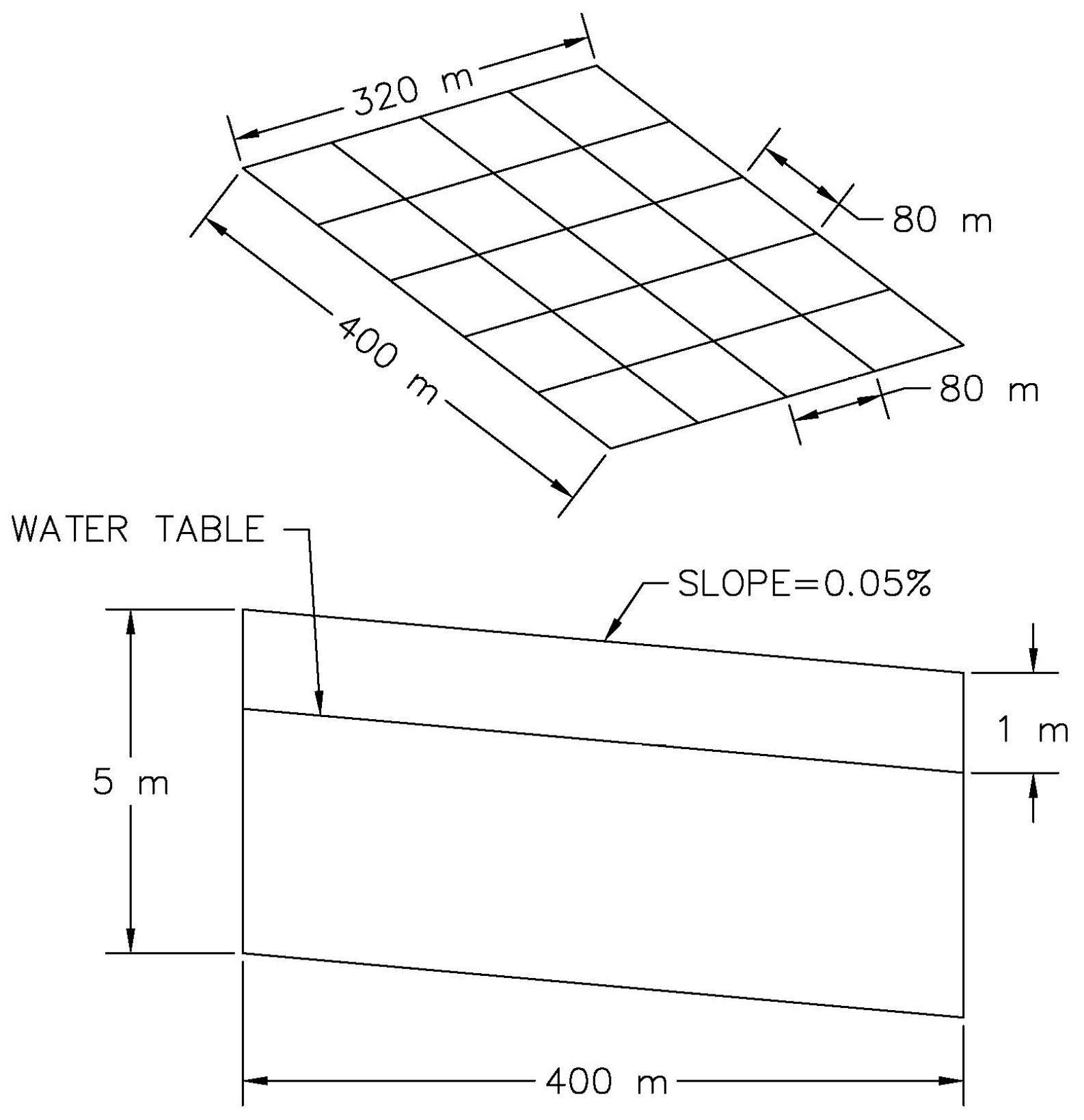
2.3.1. Infiltration Excess

The infiltration excess test case [4,15] generates runoff using a saturated hydraulic conductivity (Ks) that is much smaller than the rainfall intensity. The domain is a simple one-dimensional hillslope with a uniform soil depth of 5 m and a no flow bottom boundary condition (Figure 2). We applied a uniform rainfall of 3.3 × 10⁻⁴ m/min for 200 min followed by a 100-min recession period.

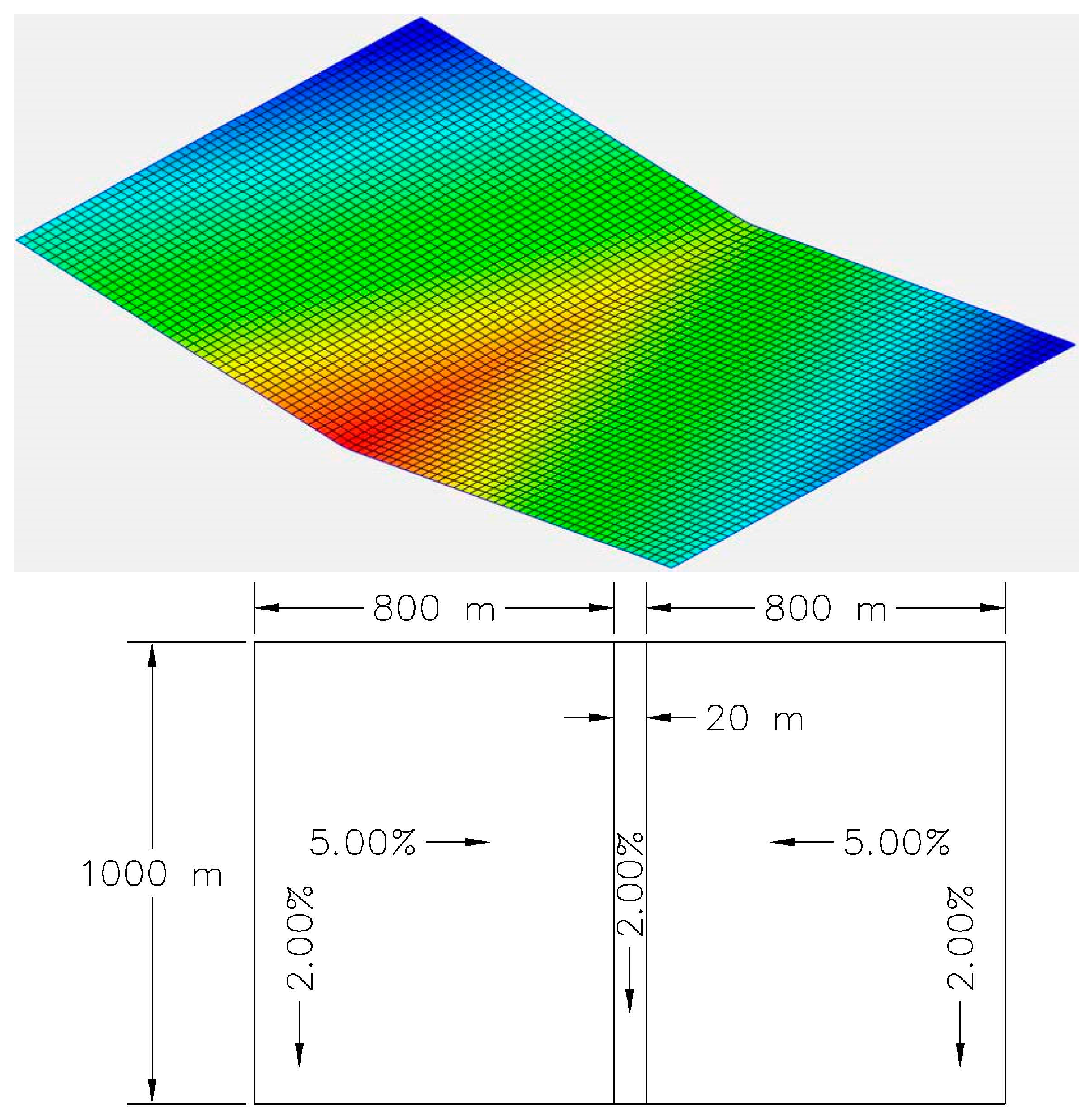
2.3.2. Tilted V-Catchment

The tilted V-catchment case evaluates the routing of each model without any infiltration or subsurface interactions. As the name implies the tilted V-catchment [4,12,13,15,50] is a v-shaped watershed formed by two inclined rectangular planes (800 m by 1000 m) connected by a channel (20 m wide) (Figure 3). We applied a uniform rainfall of 1.8 × 10⁻⁴ m/min for 90 min followed by a 90-min recession.

3. Results

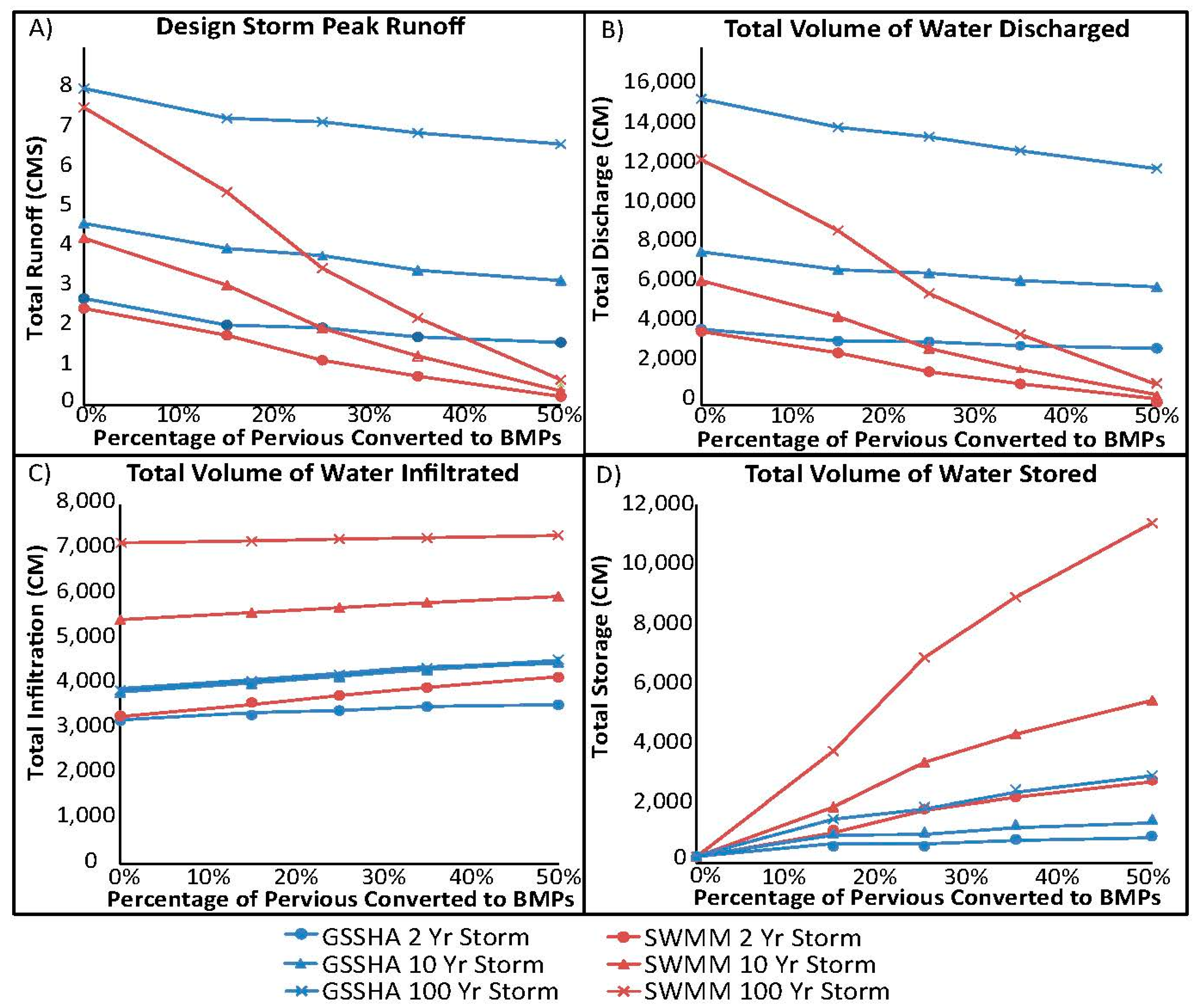
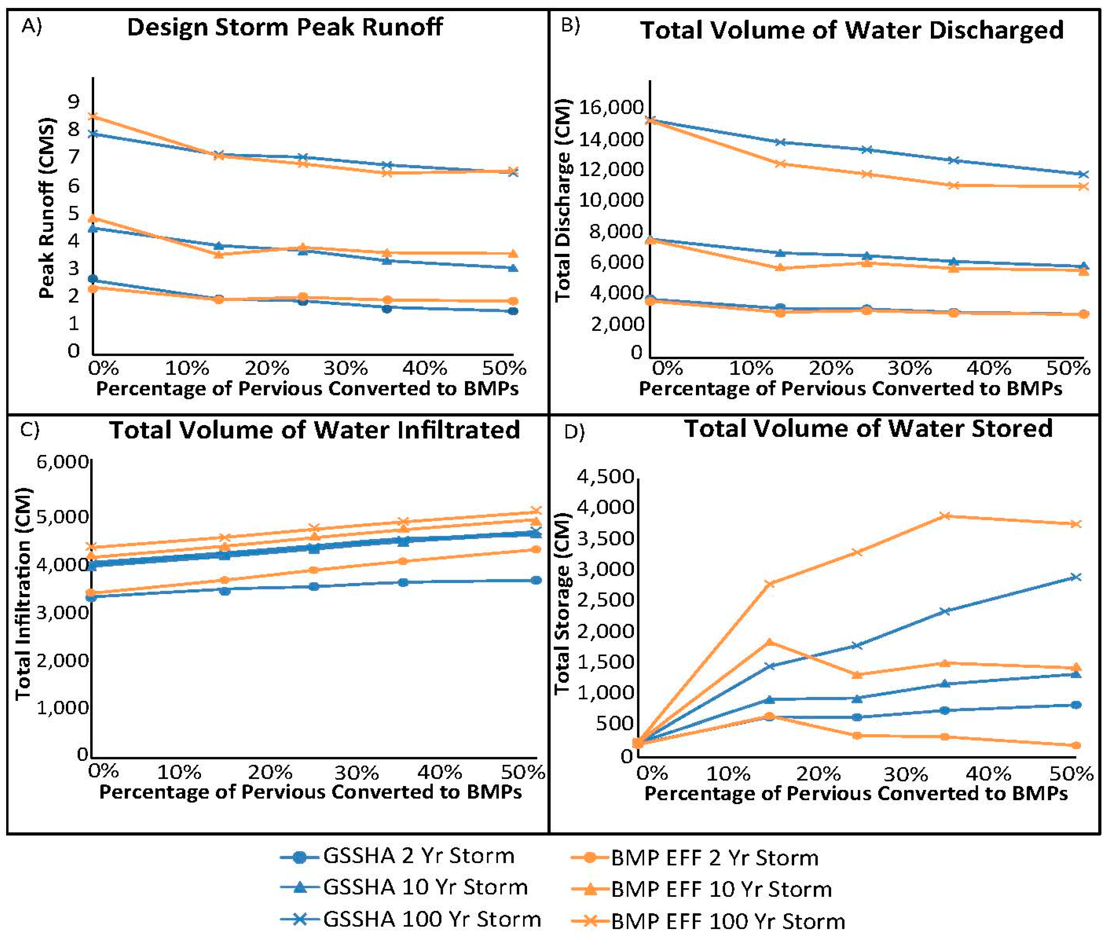
3.1. Urban Benchmark Case Study: Green Infrastructure

The urban case study comparison produces significant model disagreement. The results are shown in Figure 4. For clarity, the results are shown for only three of the five simulations (2-Year, 10-Year, and 100-Year). As described above this analysis built upon the previous modeling analysis completed by Fry and Maxwell [7].
The results show an interesting pattern, although the models were calibrated to each other for the 2-Year storm event, results between the models diverged under existing conditions as storm intensity increased (Figure 4). This is due to the difference in how each model represents runoff and infiltration and highlights the need to calibrate lumped models for each storm event.
Under each simulation for peak runoff the models diverge significantly with increasing GI, as SWMM appears to converge on a minimal peak outflow for the 50% GI simulation (Figure 4A). Peak discharge diverges 86.7% for the 2-Year storm event, and 90.4% for the 100-Year storm event. Total volume of discharge varies like peak discharge for the existing conditions simulation especially for the larger storm events (Figure 4B). Similar to peak discharge, the total volume of discharge appears to converge towards a minimal volume of discharge for the 50% GI simulation, with total discharge volume diverging 89.5% for the 2-Year Storm event, and 91.4% for the 100-Year Storm event. To understand the reasons behind the divergence between the models, an evaluation of the idealized benchmark test cases was performed.

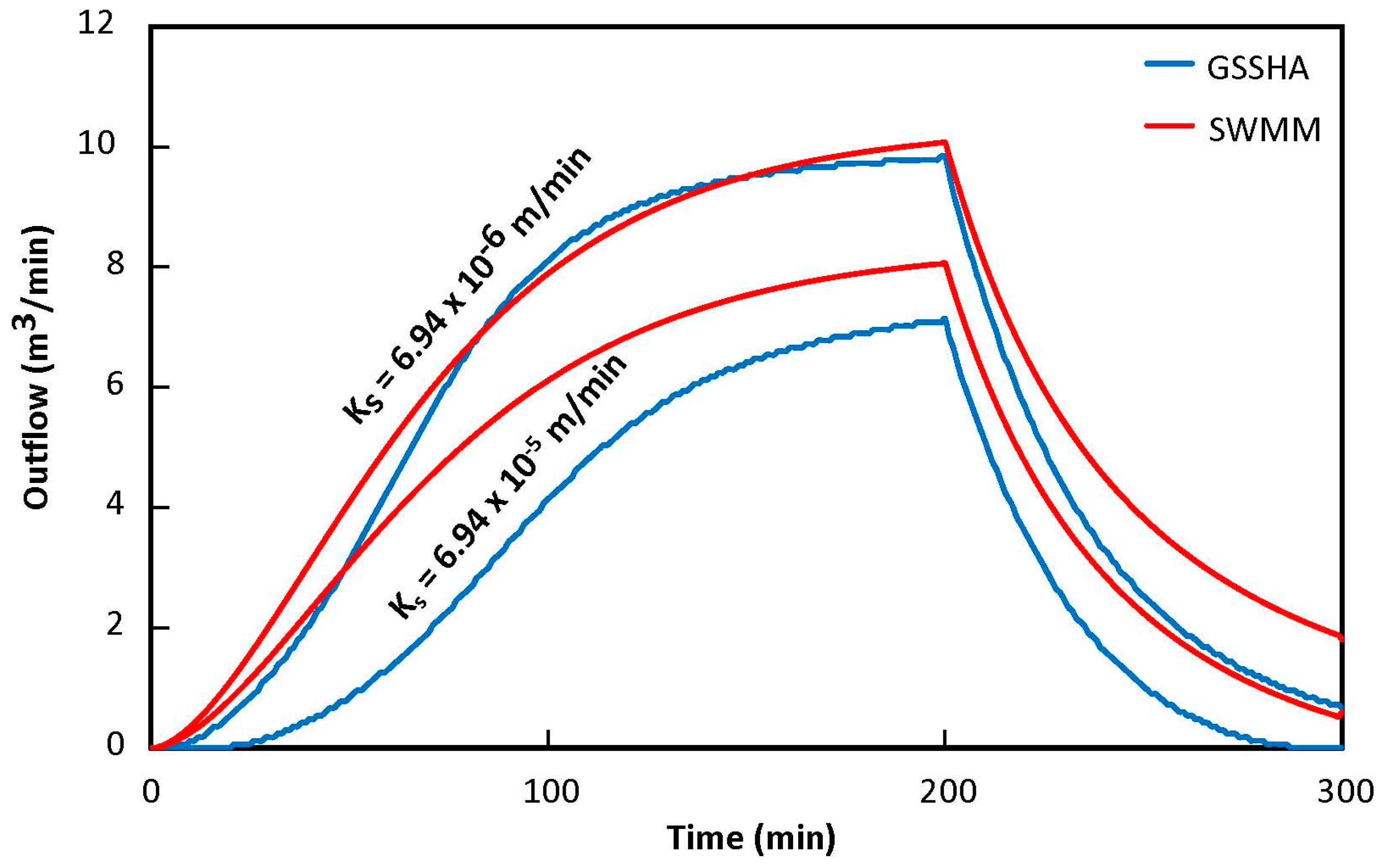
3.2. Infiltration Excess

The results of the infiltration excess benchmark case are shown in Figure 5 and provided in Table 3. The results in Figure 5 show the outflow plotted as a function of time. The plot shows good agreement for the lower Ks value with consistent outflow behavior throughout all phases of the hydrograph. There is much more divergence between the models for the higher Ks value. SWMM produces the largest peak and runoff volumes. The maximum difference between the models occurs during the recession curve (evaluated as the difference between discharges at 250 min.) and is approximately 34% for the lower Ks value and 54% for the higher Ks value.
Overall the results indicate the significant differences in each model’s capability to predict excess runoff, especially as the hydraulic conductivity increases, with SWMM predicting the least amount of infiltration in both cases. This is due to the different modeling methods, for example SWMM has lumped parameters whereas GSSHA has distributed parameters. Without some form of calibration, we anticipate that a lumped parameter model would diverge from a distributed model, and the results indicate this is the case.

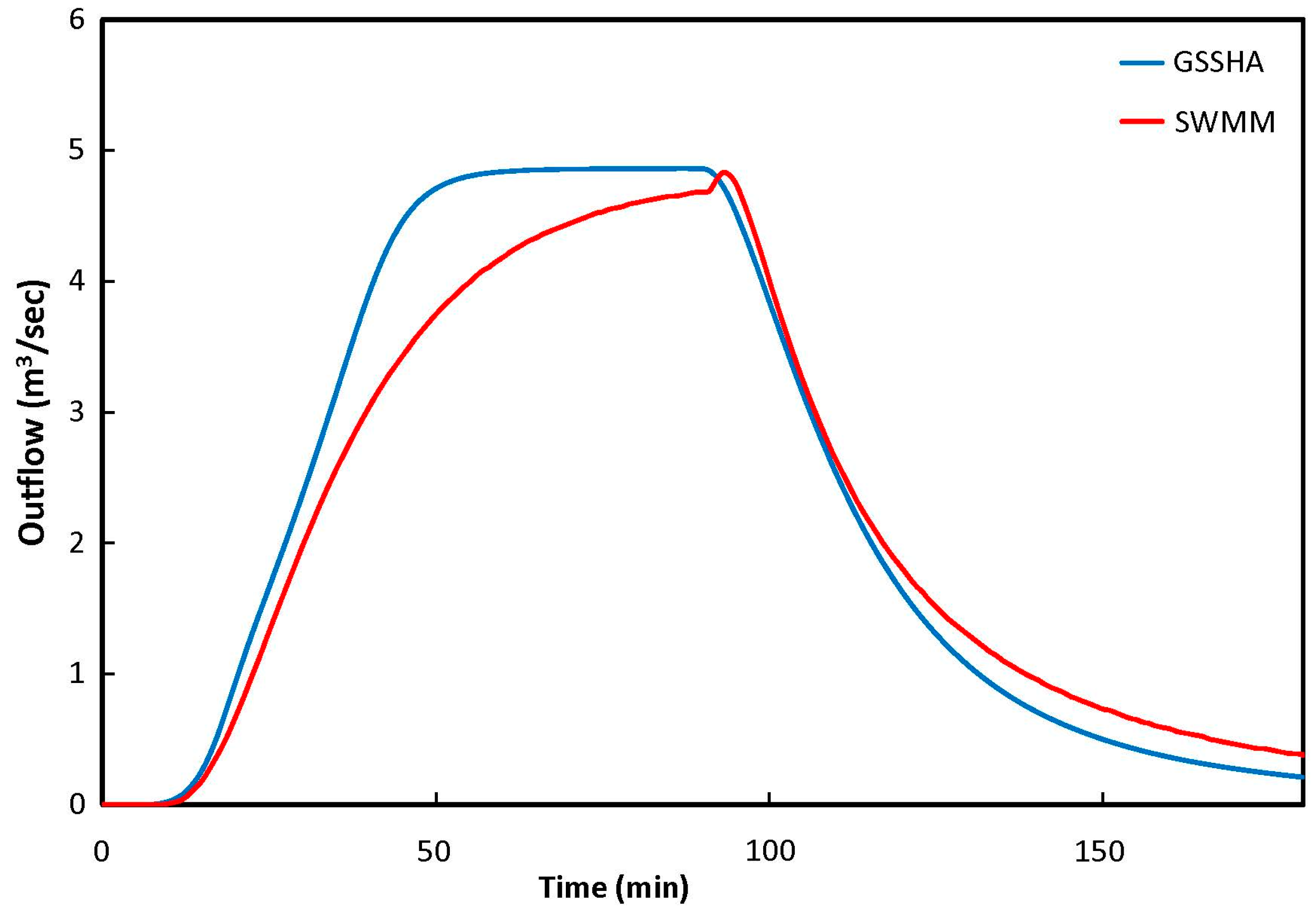
3.3. Tilted V-Catchment

We summarize the results of the Tilted V-catchment in Table 3. The outflow hydrographs are shown in Figure 6. The models predict almost identical peak outflow values (less than 1%). The predicted peak volumes are also similar for each model. The greatest difference seen is in the prediction of time to steady state, approximately 39% (as defined by an outflow area greater than 95% of the value at 90 min) between GSSHA and SWMM. There is greater agreement between the models for the recession curve (difference between discharges at 150 min) than for the rising limb.
The differences in the results are similar to previous studies and are due to the different overland and channel routing schemes used by each model [4,12,15]. The distributed model uses a form of the St. Venant equations to route overland and channel flow, whereas the lumped model uses a nonlinear reservoir method. The results indicate that this approach, if not calibrated, produces significantly different results versus the distributed model.
Based on the Tilted V-Catchment and Infiltration Excess test cases we can reason that SWMM is under predicting the outflow and over predicting the infiltration and storage volumes, thus leading to more significant reductions in peak discharge and the total volume of discharge than the GSSHA model.

4. Discussion

A review of the idealized benchmark test cases indicates good correlation between the models for the simple Infiltration Excess (low Ks). The models diverge under different infiltration parameters and overland flow routing. Even though both models use the Green Ampt method for infiltration the model structure and routing methods have a significant impact on the results. These differences point to the challenge of solving highly nonlinear runoff/run-on mechanisms [4]. These runoff processes are quite important in the application of GI in urban environments, in which surface and sub-surface interactions are more dynamic. We tend to see a large divergence between the two model types when the simulated domain became more complex and dynamic.
Our intercomparison review of the models indicates that the largest contributing factor is the difference in how the models simulate and route runoff. SWMM’s method of planes is significantly different than GSSHA, which physically routes stormwater through the built environment and the distributed GI. The SWMM method assumes that all water on a plane is completely routed through that plane minus abstractions. Therefore, the GI plane assumes all runoff routed to it is captured and treated equally. This would account for and explain the large divergence between the model results. The GSSHA’s physical routing of runoff accounts for spatial distribution of GI, as well as varied flow paths [7].
To validate this assumption, we performed an analysis in which we applied the Effective Ratio results from Fry and Maxwell [7] to the lumped model. This process consisted of using the overall Best Management Practices (BMP) Effective Ratios for each storm and percent of GI, in SWMM. Within the GI module in SWMM, the user can specify the percent of impervious area routed to the designated GI. Initially we calculated this value based on the spatial distribution of impervious areas and location of GI within the sub watershed. We replaced these values with the overall BMP Effective Ratios. We took into account that the overall BMP Effective Ratios consider both the pervious and impervious areas of the sub-watershed. Since SWMM assumes only the impervious area is routed to GI, we applied a weighted average of the BMP Effective Ratios accounting for impervious and pervious areas in the sub-watershed. In addition to more accurately represent the BMP Effectiveness Ratios, we calibrated the SWMM model to the GSSHA model for all Existing Conditions. This eliminated the bias towards divergence due to a change in storm intensity. The results are shown in Figure 7. For clarity, the results are shown for three of the five simulations (2-Year, 10-Year, and 100-Year).
Application of the BMP Effective Ratios in SWMM produced results that were more significantly consistent with the GSSHA results. These results validate that spatial location and available flow paths are highly significant for distributed GI Effectiveness at larger scales and are not easily accounted for in lumped models. The process outlined and applied here provides a framework in which modelers account for and apply physical processes from a distributed coupled model to inform lumped model parameters at the watershed scale.

5. Conclusions

This paper presents the intercomparison of a physics-based distributed hydrologic model and a lumped model using a new urban test case and a standard set of test problems. The models compared use a range of coupled strategies and varying solution techniques. Similar to Maxwell et al. [4] and Kollet et al. [17] the models produced similar results for the simpler set of test problems with the results diverging under more complex simulations. We draw some specific conclusions from this work:
  • A more complex simulation comparing existing urban conditions to proposed GI implementation was completed (Urban Case Study). This simulation compared a distributed model to a lumped model. The results showed a divergence in the model predictions of GI effectiveness. This divergence was the result of significant differences between how each type of model represents and solves the dynamic system. These results highlight the challenges of using lumped models to represent complex systems for future scenarios.
  • The models showed consistent agreement for the simple test cases focused on infiltration (infiltration excess for the low Ks value). Simple test cases can serve to build model confidence as they cover a large range of runoff generating mechanisms often encountered in catchment hydrology [4].
  • The models showed significant differences when comparing infiltration excess (high Ks value), and overland flow (Tilted-V). The different solution techniques used by each model and the increased complexity of the modeled system led to differences between the models.
  • We incorporated BMP Effectiveness Ratios [7] from the distributed model that account for the dynamics of the environment and physics of flow based on storm intensity to a lumped model to improve GI modeling accuracy. Applying the distributed model BMP Effectiveness Ratios to the lumped model produced results consistent with the distributed model. This method provides a framework with which modelers can inform and improve GI modeling within lumped models.
Although there are quantitative differences between the models for the various test cases there is qualitative agreement. While this provides confidence in all of the models in this intercomparison, it also provides an important understanding of runoff processes for each model and how we can apply these models to more complex simulations. While distributed models require substantially greater computational expense than their lumped counterparts, they appear to provide important insight into modeling green infrastructure. This class of model is an important tool for low impact urban planning.

Author Contributions

T.J.F. and R.M.M. reviewed the existing data and conceived of the experiment. T.J.F. created and ran the simulations and conducted the analysis. T.J.F. and R.M.M. collaborated on the experiment results, synthesized the data, and wrote the manuscript.

Funding

This research was funded by the U.S. National Science Foundation Engineering Research Center for Reinventing the Nation’s Urban Water Infrastructure (ReNUWIt), award number EEC-1028968.

Acknowledgments

The authors are grateful to Jeffrey Sickles, Donald Jacobs, and Enginuity Engineering Solutions for their consultation and assistance.

Conflicts of Interest

The authors declare no conflicts of interest.

References

  1. Barbosa, A.E.; Fernandes, J.N.; David, L.M. Key issues for sustainable urban stormwater management. Water Res. 2012, 46, 6787–6798. [Google Scholar] [CrossRef] [PubMed]
  2. Burns, M.J.; Fletcher, T.D.; Walsh, C.J.; Ladson, A.R.; Hatt, B.E. Hydrologic shortcomings of conventional urban stormwater management and opportunities for reform. Landsc. Urban Plan. 2012, 105, 230–240. [Google Scholar] [CrossRef]
  3. Jefferson, A.J.; Bhaskar, A.S.; Hopkins, K.G.; Fanelli, R.; Avellaneda, P.M. Stormwater management network effectiveness and implications for urban watershed function: A critical review. Hydrol. Process. 2017, 31, 4056–4080. [Google Scholar] [CrossRef]
  4. Maxwell, R.M. Surface-Subsurface model intercomparison: A first set of benchmark results to diagnose integrated hydrology and feedbacks. Water Resour. Res. 2014, 50, 1531–1549. [Google Scholar] [CrossRef]
  5. Bell, C.D.; McMillan, S.K.; Clinton, S.M.; Jefferson, A.J. Hydrologic response to stormwater control measures in urban watersheds. J. Hydrol. 2016, 541, 1488–1500. [Google Scholar] [CrossRef]
  6. Bhaskar, A.S.; Jantz, C.; Welty, C.; Drzyzga, S.A.; Miller, A.J. Coupling of the Water Cycle with Patterns of Urban Growth in the Baltimore Metropolitan Region, United States. J. Am. Water Resour. Assoc. 2016, 52, 1509–1523. [Google Scholar] [CrossRef]
  7. Fry, T.J.; Maxwell, R.M. Evaluation of Distributed BMPs in an Urban Watershed–High resolution modeling for Storm Water Management. J. Hydrol. Process. 2017. [Google Scholar] [CrossRef]
  8. Lim, T.C.; Welty, C. Effects of spatial configuration of imperviousness and green infrastructure networks on hydrologic response in a residential sewershed. Water Resour. Res. 2017, 53, 8084–8104. [Google Scholar] [CrossRef]
  9. Bosley, E.K. Hydrologic Evaluation of Low Impact Development Using a Continuous, Spatially-Distributed Model. Master’s Thesis, Virginal Polytechnic Institute and State University, Blacksburg, VA, USA, 2008. [Google Scholar]
  10. Miller, J.D.; Kim, H.; Kjeldsen, T.R.; Packman, J.; Grebby, S.; Dearden, R. Assessing the impact of urbanization on storm runoff in a peri-urban catchment using historical change in impervious cover. J. Hydrol. 2014, 15, 59–70. [Google Scholar] [CrossRef] [Green Version]
  11. Parlange, J.Y.; Rose, C.W.; Sander, G. Kinematic flow approximation of runoff on a plane: An exact analytical solution. J. Hydrol. 1981, 52, 171–176. [Google Scholar] [CrossRef]
  12. Panday, S.; Huyakorn, P.S. A fully coupled physically-based spatially-distributed model for evaluating surface/subsurface flow. Adv. Water Resour. 2004, 27, 361–382. [Google Scholar] [CrossRef]
  13. Kollet, S.J.; Maxwell, R.M. Integrated surface-groundwater flow modeling: A free-surface overland flow boundary condition in a parallel groundwater flow model. Adv. Water Resour. 2006, 29, 945–958. [Google Scholar] [CrossRef]
  14. Shen, C.; Phanikumar, M.S. A process-based, distributed hydrologic model based on a large-scale method for surface–subsurface coupling. Adv. Water Resour. 2010, 33, 1524–1541. [Google Scholar] [CrossRef]
  15. Sulis, M.; Meyerhoff, S.B.; Paniconi, C.; Maxwell, R.M.; Putti, M.; Kollet, S.J. A comparison of two physics-based numerical models for simulating surface water–groundwater interactions. Adv. Water Resour. 2010, 33, 456–467. [Google Scholar] [CrossRef]
  16. Sebben, M.L.; Werner, A.D.; Liggett, J.E.; Partington, D.; Simmons, C.T. On the testing of fully integrated surface–subsurface hydrological models. Hydrol. Process. 2013, 27, 1276–1285. [Google Scholar] [CrossRef]
  17. Kollet, S. The integrated hydrologic model intercomparison project, IH-MIP2: A second set of benchmark results to diagnose integrated hydrology and feedbacks. Water Resour. Res. 2017, 53, 867–890. [Google Scholar] [CrossRef] [Green Version]
  18. Bhaduri, B.; Harbor, J.; Engel, B.; Grove, M. Assessing watershed-scale long-term hydrologic impacts of land-use change using GIS-NPS model. Environ. Manag. 2000, 26, 643–658. [Google Scholar] [CrossRef] [PubMed]
  19. Khader, O.; Montalto, F.A. Development and calibration of a high resolution SWMM model for simulating the effects of LID retrofits on the outflow hydrograph of a dense urban watershed. Int. Low Impact Dev. Conf. 2008. [Google Scholar] [CrossRef]
  20. Lee, G.L.; Heaney, J.P. Estimation of urban imperviousness and its impacts on stormwater system. J. Water Resour. Plan. Manag. 2003, 129, 419–428. [Google Scholar] [CrossRef]
  21. Krebs, G.; Kokkonen, T.; Valtanen, M.; Setala, H.; Koivusalo, H. Spatial resolution considerations for urban hydrological modelling. J. Hydrol. 2014, 512, 482–497. [Google Scholar] [CrossRef]
  22. Elliott, A.H.; Trowsdale, S.A. A review of models for low impact urban stormwater drainage. Environ. Model. Softw. 2007, 22, 394–405. [Google Scholar] [CrossRef]
  23. Henderson-Sellers, A.; Pitman, A.J.; Love, P.K.; Irannejad, P.; Chen, T.H. The Project for Intercomparison of Land Surface Parameterization Schemes (PILPS): Phase 2 and 3. Bull. Am. Meteorol. Soc. 1995, 76, 489–503. [Google Scholar] [CrossRef]
  24. Yang, Z.L.; Dickinson, R.E.; Henderson-Sellers, A.; Pitman, A.J. Preliminary study of spin-up processes in land-surface models with the first stage data of Project for Intercomparison of Land Surface Parameterization Schemes Phase 1(a). J. Geophys. Res. 1995, 100, 16553–16578. [Google Scholar] [CrossRef]
  25. Chen, T.H. Cabauw experimental results from the Project for Intercomparison of land-surface parameterizations schemes. J. Clim. 1997, 10, 1194–1215. [Google Scholar] [CrossRef]
  26. Qu, W. Sensitivity of latent heat flux from PILPS land-surface schemes to perturbations of surface air temperature. J. Atmos. Sci. 1998, 55, 1909–1927. [Google Scholar] [CrossRef]
  27. Wood, E. The Project for Intercomparison of Land-surface Parameterization Schemes PILPS/phase 2c/Red-Arkansas River basin experiment. 1: Experiment description and summary intercomparisons. Glob. Planet. Chang. 1998, 19, 115–135. [Google Scholar] [CrossRef]
  28. Luo, L.; Robock, A. Effects of frozen soil on soil temperature, spring infiltration, and runoff: Results from the PILPS 2(d) Experiment at Valdai, Russia. J. Hydrometeorol. 2003, 4, 334–351. [Google Scholar] [CrossRef]
  29. Reed, S.; Koren, V.; Smith, M.; Zhang, Z.; Moreda, F.; Seo, D.J.; DMIP Participants. Overall distributed model intercomparison project results. J. Hydrol. 2004, 298, 27–60. [Google Scholar] [CrossRef]
  30. Smith, M.B.; Seo, D.J.; Koren, V.I.; Reed, S.M.; Zhang, Z.; Duan, Q.Y.; Moreda, F.; Cong, S. The distributed model intercomparison project (DMIP): Motivation and experiment design. J. Hydrol. 2004, 298, 4–26. [Google Scholar] [CrossRef]
  31. Downer, C.W.; Ogden, F.L.; U.S. Army Corps of Engineers. Gridded Surface Subsurface Hydrologic Analysis (GSSHA) User’s Manual, Version 11,43 for Watershed Modeling System 6.1; Engineer Research and Development Center: Vicksburg, MS, USA, 2006; p. 207.
  32. Green, W.H.; Ampt, G.A. Studies on soil physics, part I: The flow of air and water through soils. J. Agric. Sci. 1911, 4, 1–24. [Google Scholar]
  33. Ogden, F.L.; Saghafian, B. Green and Ampt infiltration with redistribution. J. Irrig. Drain. Eng. 1997, 123, 386–393. [Google Scholar] [CrossRef]
  34. Downer, C.W.; Ogden, F.L. Prediction of runoff and soil moistures at the watershed scale: Effects of model complexity and parameter assignment. Water Resour. Res. 2003, 39, 1045. [Google Scholar] [CrossRef]
  35. Rossman, L.A. Storm Water Management Model Reference Manual Volume I–Hydrology (Revised); U.S. EPA Office of Research and Development: Cincinnati, OH, USA, 2016.
  36. Rossman, L.A. Stormwater Management Model User Manual Version 5.1; U.S. Environmental Protection Agency Office of Research and Development: Cincinnati, OH, USA, 2015.
  37. Gironas, J.; Roesner, L.A.; Davis, J. Storm Water Management Model Applications Manual; National Risk Management Research Laboratory Office of Research and Development, U.S. Environmental Protection Agency: Cincinnati, OH, USA, 2009.
  38. Yao, L.; Chen, L.; Wei, W. Assessing the effectiveness of imperviousness on stormwater runoff in micro urban catchments by model simulation. Hydrol. Process. 2015. [Google Scholar] [CrossRef]
  39. Yao, L.; Wei, W.; Chen, L. How does imperviousness impact the urban rainfall-runoff process under various storm cases? Ecol. Indic. 2016, 60, 893–905. [Google Scholar] [CrossRef] [Green Version]
  40. Urban Drainage and Flood Control District. Urban Drainage and Flood Control District Criteria Manual 1; Urban Drainage and Flood Control District: Denver, CO, USA, 2016.
  41. City and County of Denver. Geographic Information System; City and County of Denver: Denver, CO, USA, 2014. [Google Scholar]
  42. Engman, T. Roughness Coefficients for Routing Surface Runoff. J. Irrig. Drain. Eng. 1986, 112, 39–53. [Google Scholar] [CrossRef]
  43. McCuen, R.; Johnson, P.; Ragan, R. Hydrology; Federal Highway Administration: Washington, DC, USA, 1996.
  44. McCuen, R.; Johnson, P.; Ragen, R. Highway Hydrology, 2nd ed.; Hydraulic Design Series No. 2; US Department of Transportation: Washington, DC, USA, 2002; Chapter 5; pp. 24–28.
  45. Rawls, W.J.; Brakensiek, D.L. A Procedure to Predict Green and Ampt Infiltration Parameters. In Proceedings of the ASAE Conference on Advances in Infiltration, Chicago, IL, USA, 12–13 December 1983; pp. 102–112. [Google Scholar]
  46. Rawls, W.J.; Brakensiek, D.L. Prediction of soil water properties for hydrologic modeling. In Symposium on Watershed Management in the Eighties; Jones, E.B., Ward, T.J., Eds.; American Society of Cicil Engineers: New York, NY, USA, 1985; pp. 293–399. [Google Scholar]
  47. Natural Resources Conservation Service. Soil Survey Data; US Department of Agriculture: Washington, DC, USA, 2014.
  48. City and County of Denver. Ultra-Urban Green Infrastructure Guidelines; City and County of Denver Public Works: Denver, CO, USA, 2016. [Google Scholar]
  49. Urban Drainage and Flood Control District. Urban Drainage and Flood Control District Criteria Manual 3; Urban Drainage and Flood Control District: Denver, CO, USA, 2016.
  50. Gottardi, G.; Venutelli, M. A control-volume finite-element model for two-dimensional overland flow. Adv. Water Resour. 1993, 16, 277–284. [Google Scholar] [CrossRef]
  51. Kumar, M.; Duffy, C.J.; Salvage, K.M. A second order accurate, finite volume based, integrated hydrologic modeling (FIHM) framework for simulation of surface and subsurface flow. Vadose Zone J. 2009, 8, 873–890. [Google Scholar] [CrossRef]
Figure 1. Urban case domain. (A) Example set up of urban mask with 15% green infrastructure (GI) placement; (B) Surface elevations based upon City and County of Denver 2008 Lidar Data.
Water 10 01756 g001
Figure 2. Infiltration Excess test case domain [15].
Water 10 01756 g002
Figure 3. Tilted V-Catchment test case domain [4,13,15].
Water 10 01756 g003
Figure 4. Green Infrastructure comparison results. Gridded Surface Subsurface Hydrologic Analysis (GSSHA) results are presented in blue, and Storm Water Management Model (SWMM) results are presented in red for each simulation and storm event. The results are presented for: Peak Runoff (A); Runoff Volume (B); Total Infiltration Volume (C); and Total Storage (D).
Water 10 01756 g004
Figure 5. Outflow hydrograph response of the Infiltration Excess test case with two values of saturated hydraulic conductivity.
Water 10 01756 g005
Figure 6. Tilted V-Catchment outflow hydrographs.
Water 10 01756 g006
Figure 7. Green Infrastructure comparison results with the BMP Effectiveness Ratios applied in SWMM. GSSHA results are presented in blue, and SWMM with BMP Effectiveness ratios are presented in orange for each simulation and storm event. The results are presented for: Peak Runoff (A); Runoff Volume (B); Total Infiltration Volume (C); and Total Storage (D). The results indicate that application of BMP Effective ratios in SWMM produced results that are consistent with GSSHA.
Water 10 01756 g007
Table 1. Parameter values used in the urban benchmark case: green infrastructure.
Neighborhood Subset CharacteristicsValueUnitsSource
Total Area261,422m2City and County of Denver
Geographic Information system (GIS) (2014) [41]
Impervious Areas137,427m2
Pervious Areas123,995m2
Native Soil Properties
Hydraulic Conductivity0.06cm/hEngman (1986) [42]; McCuen et al. (1996 and 2002) [43,44];
Capillary Head32cmRawls and Brakensiek (1983 and 1985) [45,46];
US Natural Resources Conservation Service (NRCS)
Porosity0.4cm3/cm3Soil Survey Data (soils.usda.gov/survey) [47]
Residual Saturation0.165cm3/cm3
Field Capacity0.09cm3/cm3
Wilting Point0.4cm3/cm3
Initial Moisture0.27%
Surface Roughness Values
Impervious Areas0.015 Engman (1986) [42]; McCuen et al. (1996 and 2002) [43,44]
Pervious Areas0.04
GI Soil Properties
Hydraulic Conductivity1.09cm/hCity of Denver Ultra Urban Manual
Capillary Head11.01cm(2016) [48]; Urban Drainage and Flood Control District (UDFCD)
Vol. III (2016) [49]
Porosity0.412cm3/c3
Residual Saturation0.041cm3/cm3
Field Capacity0.207cm3/cm3
Wilting Point0.095cm3/cm3
Initial Moisture0.358%
GI Characteristics
Surface Storage Depth304.8mmUDFCD Vol. III (2016) [49]
Table 2. Parameter values used in the benchmark cases.
Parameter Values for Benchmark Cases
Units1. Infiltration Excess2. Tilted V-Catchment
Saturated Hydraulic ConductivityKsm/min6.94 × 10−5 (High K)a
m/min6.94 × 10−6 (Low K)a
Manning’s Roughnessn 0.019860.015 (Hillslope)
0.15 (Channel)
Rainfall Rateim/min3.30 × 10−41.80 × 10⁻⁴
Specific StorageSs1/m5 × 10−45 × 10−4
PorosityΦ 0.40.4
van Genuchten Parameters
Alphaα1/cm1.01.0
Pore-size distributionsn-2.02.0
Residual water contentSres-0.20.2
Saturated water contentSsat-1.01.0
Green Ampt Parameters
Capillary HeadΨcm16.716.7
Pore Distribution Indexλ-2.02.0
Residual Saturationθr-0.20.2
Field Capacityθf-0.40.4
Wilting Pointθwp-0.150.15
a The Tilted V-Catchment case is surface flow only.
Table 3. Summary metrics for benchmark cases by model.
Infiltration Excess Ks = 0.01Infiltration Excess Ks = 0.1Tilted V-Catchment
QpeaktpeakVolumeQpeaktpeakVolumeQpeaktpeakVolume
GSSHA0.164199.8016220.119200.009244.86085.0025,417
SWMM0.170199.8017770.134200.0013254.83093.0024,065
Qpeak is the peak flow in m3/s, tpeak is the time of peak flow in min. Volume is in m3.

