Improved Soil Temperature Modeling Using Spatially Explicit Solar Energy Drivers

Abstract
:1. Introduction
2. Materials and Methods
2.1. Previous Solar and Generalized Soil Modeling Methods
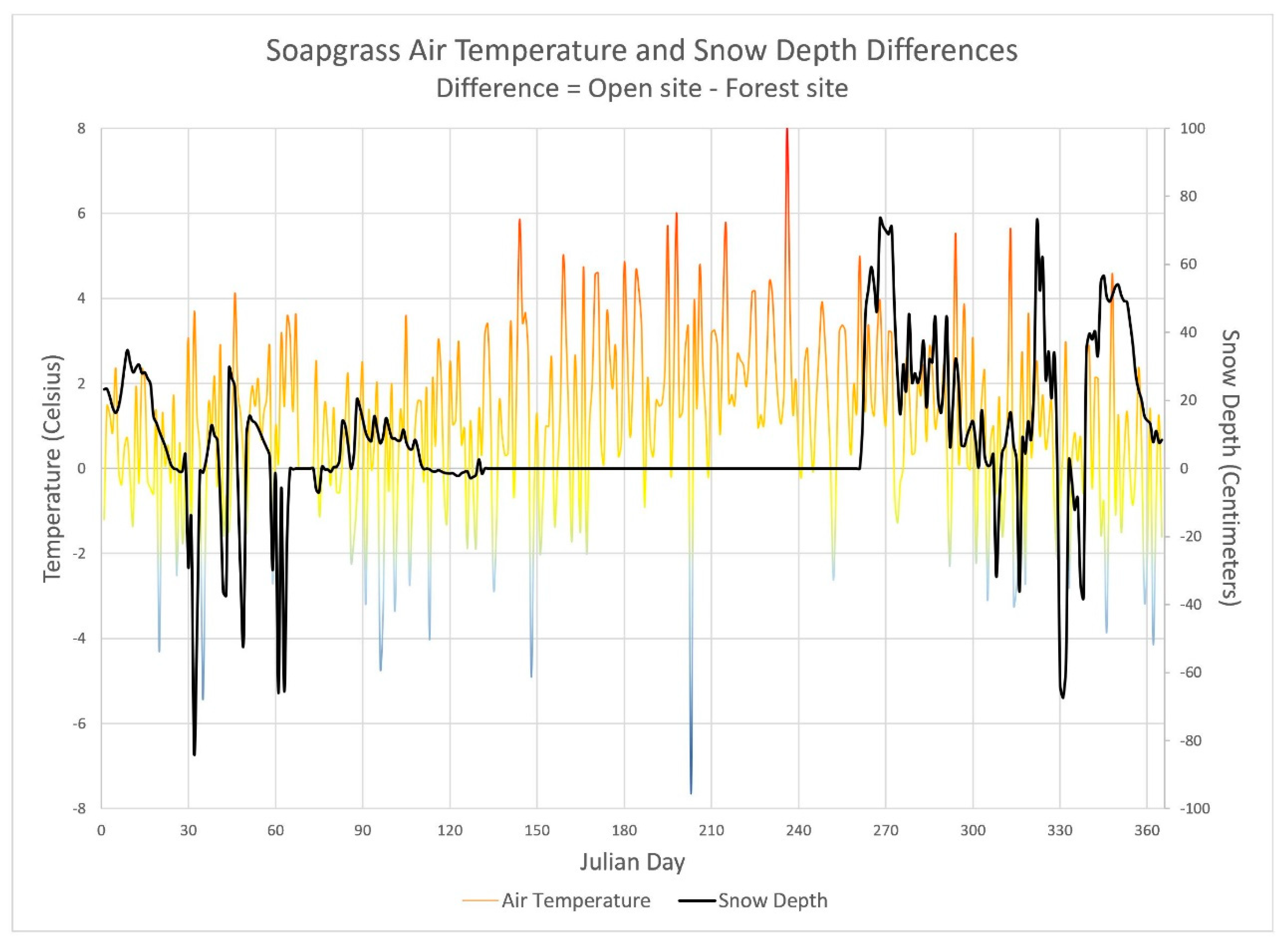
2.2. Soil Temperature Variations Due to Landscape Coverage
2.3. Original VELMA Air Soil Temperature (AST) Subroutine
2.4. New VELMA Air Soil Temperature-Solar (AST-Solar) Subroutine
2.5. Subroutine Testing
2.5.1. O’CCMoN Testing Sites
2.5.2. AST versus AST-Solar Subroutine Setup
3. Results
4. Discussion
5. Conclusions
Author Contributions
Funding
Conflicts of Interest
References
- Mayer, T.D. Controls of Summer Stream Temperature in the Pacific Northwest. J. Hydrol. 2012, 475, 323–335. [Google Scholar] [CrossRef]
- Reich, P.B.; Luo, Y.; Bradford, J.B.; Poorter, H.; Perry, C.H.; Oleksyn, J. Temperature drives global patterns in forest biomass distribution in leaves, stems, and roots. Proc. Natl. Acad. Sci. USA 2014, 111, 13721–13726. [Google Scholar] [CrossRef] [PubMed] [Green Version]
- Mellander, P.-E.; Stähli, M.; Gustafsson, D.; Bishop, K. Modelling the effect of low soil temperatures on transpiration by Scots pine. Hydrol. Process. 2006, 20, 1929–1944. [Google Scholar] [CrossRef]
- Stieglitz, M.; Ducharne, A.; Koster, R.; Suarez, M. The impact of detailed snow physics on the simulation of snow cover and subsurface thermodynamics at continental scales. J. Hydrometeorol. 2001, 2, 228–242. [Google Scholar] [CrossRef]
- Abdelnour, A.; Stieglitz, M.; Pan, F.; Mckane, R. Catchment hydrological responses to forest harvest amount and spatial pattern. Water Resour. Res. 2011, 47, 1995–2021. [Google Scholar] [CrossRef]
- Neitsch, S.L.; Arnold, J.G.; Kiniry, J.R.; Williams, J.R.; King, K.W. Soil and Water Assessment Tool Theoretical Documentation Version 2009; Texas Water Resources Institute, Texas A&M University System: College Station, TX, USA, 2011; pp. 32–38. [Google Scholar]
- Tague, C.L.; Band, L.E. RHESSys: Regional hydro-ecologic simulation system—An object-oriented approach to spatially distributed modeling of carbon, water, and nutrient cycling. Earth Interact. 2004, 8, 1–42. [Google Scholar] [CrossRef]
- Bicknell, B.R.; Imhoff, J.C.; Kittle, J.L.; Donigian, A.S.; Johanson, R.C. Hydrological Simulation Program—Fortran, User’s Manual for Version 11; U.S. Environmental Protection Agency, National Exposure Research Laboratory: Athens, GA, USA, 1997; p. 755.
- National Weather and Climate Center (NWCC). Snow Telemetry (SNOTEL) Data Collection Network; Natural Resources Conservation Service (NRCS): Portland, OR, USA, 2016.
- Reynolds, C.J., III. Aviation Weather Information Dissemination System. U.S. Patent 4,521,857, 4 June 1985. [Google Scholar]
- Foundation, N.S. LTER Network. Available online: https://lternet.edu/ (accessed on 26 September 2018).
- OSU Research Forests. Available online: http://cf.forestry.oregonstate.edu/ (accessed on 26 September 2018).
- Harvard Forest. Available online: https://harvardforest.fas.harvard.edu/ (accessed on 26 September 2018).
- Fuka, D.R.; Walter, M.T.; MacAlister, C.; Degaetano, A.T.; Steenhuis, T.S.; Easton, Z.M. Using the Climate Forecast System Reanalysis as weather input data for watershed models. Hydrol. Process. 2013, 28, 5613–5623. [Google Scholar] [CrossRef]
- Daly, C.; Halbleib, M.; Smith, J.I.; Gibson, W.P.; Doggett, M.K.; Taylor, G.H.; Curtis, J.; Pasteris, P.P. Physiographically sensitive mapping of climatological temperature and precipitation across the conterminous United States. Int. J. Climatol. 2008, 28, 2031–2064. [Google Scholar] [CrossRef] [Green Version]
- Thornton, P.E.; Running, S.W.; White, M.A. Generating surfaces of daily meteorological variables over large regions of complex terrain. J. Hydrol. 1997, 190, 214–251. [Google Scholar] [CrossRef] [Green Version]
- Staff, S.S.D. Soil survey manual. In USDA Handbook 18; Ditzler, C., Scheffe, K., Monger, H.C., Eds.; Government Printing Office: Washington, DC, USA, 2017. [Google Scholar]
- Li, G.; Jackson, C.R.; Kraseski, K.A. Modeled riparian stream shading: Agreement with field measurements and sensitivity to riparian conditions. J. Hydrol. 2012, 428–429, 142–151. [Google Scholar] [CrossRef]
- Boyd, M.; Kasper, B. Analytical Methods for Dynamic Open Channel Heat and Mass Transfer: Methodology for the Heat Source Model Version 7.0; Watershed Sciences Inc.: Portland, OR, USA, 2003. [Google Scholar]
- Seidl, R.; Rammer, W.; Scheller, R.M.; Spies, T.A. An individual-based process model to simulate landscape-scale forest ecosystem dynamics. Ecol. Model. 2012, 231, 87–100. [Google Scholar] [CrossRef]
- Chiacchio, M.; Solmon, F.; Giorgi, F.; Stackhouse, P.; Wild, M. Evaluation of the radiation budget with a regional climate model over Europe and inspection of dimming and brightening. J. Geophys. Res. Atmos. 2015, 120, 1951–1971. [Google Scholar] [CrossRef] [Green Version]
- Alexandri, G.; Georgoulias, A.K.; Zanis, P.; Katragkou, E.; Tsikerdekis, A.; Kourtidis, K.; Meleti, C. On the ability of RegCM4 regional climate model to simulate surface solar radiation patterns over Europe: An assessment using satellite-based observations. Atmos. Chem. Phys. 2015, 15, 13195–13216. [Google Scholar] [CrossRef]
- Waschmann, R.S.; U.S. Environmental Protection Agency—Western Ecology Division. Oregon Crest-to-Coast Climate Observations; NOAA National Centers for Environmental Information: Corvallis, OR, USA, 2014.
- Ficklin, D.L.; Luo, Y.; Stewart, I.T.; Maurer, E.P. DeveloFpment and application of a hydroclimatological stream temperature model within the Soil and Water Assessment Tool. Water Resour. Res. 2012, 48. [Google Scholar] [CrossRef]
- Bokhorst, S.; Huiskes, A.; Aerts, R.; Convey, P.; Cooper, E.J.; Dalen, L.; Erschbamer, B.; Gudmundsson, J.; Hofgaard, A.; Hollister, R.D.; et al. Variable temperature effects of Open Top Chambers at polar and alpine sites explained by irradiance and snow depth. Glob. Chang. Biol. 2012, 19, 64–74. [Google Scholar] [CrossRef] [PubMed]
- McKane, R.B.; Brookes, A.; Djang, K.; Stieglitz, M.; Abdelnour, A.G.; Pan, F.; Halama, J.J.; Pettus, P.B.; Phillips, D.L. VELMA Version 2.0: User Manual and Technical Documentation; U.S. Environmental Protection Agency—Western Ecology Division: Corvallis, OR, USA, 2014; p. 60.
- Carslaw, H.S.; Jaeger, J.C. Conduction of Heat in Solids, 2nd ed.; Clarendon Press: Oxford, UK, 1959. [Google Scholar]
- Waschmann, R.S. EPA Oregon Crest to Coast Overview, Figure 2; NOAA National Centers for Environmental Information: Corvallis, OR, USA, 2018; p. 16.
- Daly, C. 30-Year Normals. Available online: http://www.prism.oregonstate.edu/normals/ (accessed on 26 September 2018).
- Halama, J.J. Penumbra: A Spatiotemporal Shade-Irradiance Analysis Tool with External Model Integration for Landscape Assessment, Habitat Enhancement, and Water Quality Improvement. Ph.D. Thesis, Oregon State University, Corvallis, OR, USA, 2017. [Google Scholar]
- Halama, J.J.; Kennedy, R.E.; Graham, J.J.; McKane, R.B.; Barnhart, B.L.; Djang, K.; Pettus, P.B.; Brookes, A.; Wingo, P.C. Penumbra: A spatially-distributed shade percent and incident ground-level irradiance model for simulating landscape scale solar energy. PLoS ONE 2018, in press. [Google Scholar]


| AST Variables | Descriptions |
| AirAVETEMP | Fixed value of 8.2 (°C) |
| AirLAG | Historic air temperature derived from the PhaseLAG. |
| LSDEPTH | Soil column depth to center (mm) per layer of interest |
| LTDACCUMULATION | Summation of the thermal deltas per layer of interest |
| SoilBELOW | Soil layer below the current layer being calculated |
| AST-Solar Variables | Descriptions |
| AirTEMP | Daily average air temperature in the open site |
| SoilAVE_TEMP | Two-day running average (°C) |
| ReducerSOLAR | Derived value from the input solar energy data |
| LayerSM | Volume to volume soil moisture level |
| SoilTemp(JDAY) | Current time steps soil temperature value |
| SoilTemp(JDAY−1) | Prior time steps soil temperature value |
| Site Name | Elevation (m) | Vegetative State | Annual Rainfall (cm) | Tree Height (m) | Soil Parent Material |
|---|---|---|---|---|---|
| Cascade Head: Open (CHO) | 157 | Lawn | 200–250 | - | Marine Sediment |
| Cascade Head: Forest (CH14) | 190 | Alder Douglas-fir Sitka Spruce | 50–60 | ||
| Moose Mountain: Open (MMO) | 668 | Clear-cut | 150–180 | - | Volcanic |
| Moose Mountain: Forest (MMF) | 658 | Douglas-fir | 50–60 | ||
| Soapgrass: Open (SGO) | 1298 | Clear-cut | 180–200 | - | Volcanic |
| Soapgrass: Forest (SGF) | 1190 | Douglas-fir | 60–70 | ||
| Toad Creek: Open (TCO) | 1202 | Clear-cut | 180–200 | - | Volcanic |
| Toad Creek: Forest (TCF) | 1198 | Douglas-fir | 50–60 |
| O’CCMoN Location | Sites | Soil Layer 1 | Soil Layer 2 | ||
|---|---|---|---|---|---|
| AST (r2) | AST3 (r2) | AST (r2) | AST3 (r2) | ||
| Cascade Head | Open Site (CHO) | 0.83 | 0.76 | 0.71 | 0.95 |
| Forest Site (CH14) | 0.74 | 0.87 | 0.71 | 0.94 | |
| Moose Mountain | Open Site (MMO) | 0.81 | 0.92 | 0.67 | 0.93 |
| Forest Site (MMF) | 0.89 | 0.93 | 0.70 | 0.94 | |
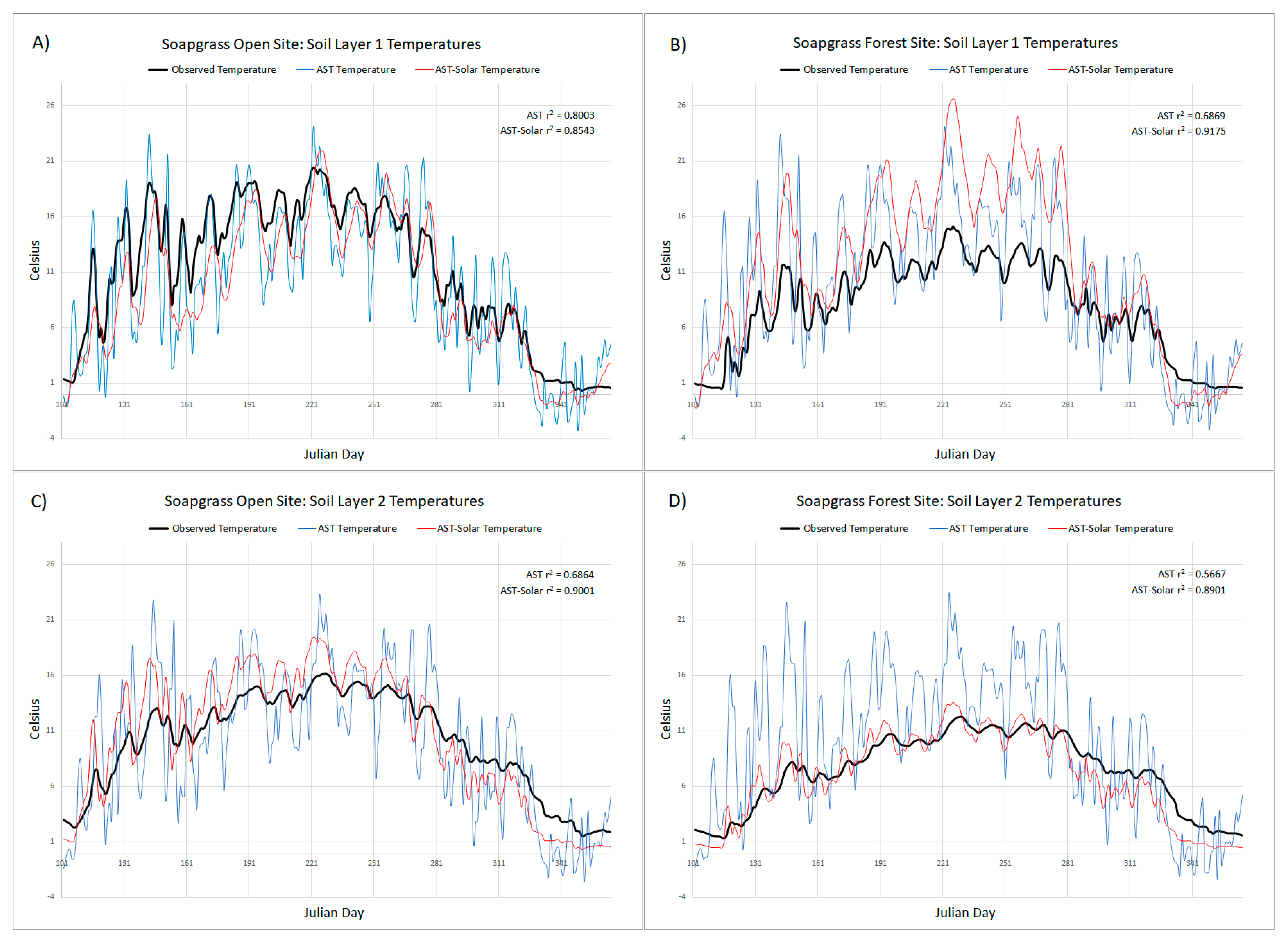
| Soapgrass | Open Site (SGO) | 0.80 | 0.85 | 0.69 | 0.90 |
| Forest Site (SGF) | 0.69 | 0.92 | 0.57 | 0.89 | |
| Toad Creek | Open Site (TCO) | 0.82 | 0.83 | 0.72 | 0.92 |
| Forest Site (TCF) | 0.83 | 0.90 | 0.64 | 0.89 | |
© 2018 by the authors. Licensee MDPI, Basel, Switzerland. This article is an open access article distributed under the terms and conditions of the Creative Commons Attribution (CC BY) license (http://creativecommons.org/licenses/by/4.0/).
Share and Cite
Halama, J.J.; Barnhart, B.L.; Kennedy, R.E.; McKane, R.B.; Graham, J.J.; Pettus, P.P.; Brookes, A.F.; Djang, K.S.; Waschmann, R.S. Improved Soil Temperature Modeling Using Spatially Explicit Solar Energy Drivers. Water 2018, 10, 1398. https://doi.org/10.3390/w10101398
Halama JJ, Barnhart BL, Kennedy RE, McKane RB, Graham JJ, Pettus PP, Brookes AF, Djang KS, Waschmann RS. Improved Soil Temperature Modeling Using Spatially Explicit Solar Energy Drivers. Water. 2018; 10(10):1398. https://doi.org/10.3390/w10101398
Chicago/Turabian StyleHalama, Jonathan J., Bradley L. Barnhart, Robert E. Kennedy, Robert B. McKane, James J. Graham, Paul P. Pettus, Allen F. Brookes, Kevin S. Djang, and Ronald S. Waschmann. 2018. "Improved Soil Temperature Modeling Using Spatially Explicit Solar Energy Drivers" Water 10, no. 10: 1398. https://doi.org/10.3390/w10101398