Prediction of Water Inflow in Subsea Tunnels under Blasting Vibration

Geotechnical and Structural Engineering Research Center, Shandong University, Ji’nan 250061, China
*
Author to whom correspondence should be addressed.
Water 2018, 10(10), 1336; https://doi.org/10.3390/w10101336
Submission received: 6 August 2018
/
Revised: 1 September 2018
/
Accepted: 18 September 2018
/
Published: 27 September 2018
(This article belongs to the Section Hydraulics and Hydrodynamics)
Abstract
:The subsea tunnel of Qingdao metro line 1 has been excavated using the drill and blast method. Blasting vibration during tunneling may cause larger water inflow and even severe security risks and considerable economic losses. However, the prediction of water inflow in subsea tunnels under blasting vibration still remains a challenging problem. Thus, this paper proposes an approach combining tests and numerical calculations for analyzing this problem. The approach is developed by analyzing the mechanical and deformation characteristics of the surrounding rock through a laboratory triaxial compression test and then establishing the strain softening constitutive model of the surrounding rock. Based on the elastic compression theory of porous media and the cubic law of fractured rock mass, we establish and analyze the evolution model of the permeability characteristics during the damage process of the surrounding rock. Then, a Fast Lagrangian Analysis of Continua in 3 Dimensions (FLAC3D) is used to verify the rationality and accuracy of the model. According to the actual blasting design scheme, the surrounding rock constitutive model, and the permeability characteristic evolution model, the blasting process and water inflow of the subsea tunnel is simulated. The amount of water inflow in the subsea tunnel calculated by using the permeability coefficient under blasting vibration (PCuBV) is compared with the measured water inflow and the amount of water inflow calculated by using the exploration permeability coefficient (EPC) and the initial permeability coefficient (IPC) of the surrounding rock. The results show that the prediction of water inflow quantity under blasting vibration is both closer to reality and more reasonable than existing models.
1. Introduction
The subsea tunnel of Qingdao metro line 1 in China is the most important traffic line connecting Qingdao to Huangdao. It is part of the recent Qingdao Metro Line Planning Network, which aims to alleviate road traffic in order to improve the quality and duration of travel. Compared to conventional on-shore tunnels, subsea tunnels involve greater risk due to the less-detailed knowledge about the geology and rock mass properties in the planning phase. The tunnel was planned in a V-shaped trend, which prevents or hinders natural drainage. The Huangdao section was constructed with the conventional drill and blast method, which may cause damage to surrounding rock and increase its permeability.
Parallel to the mechanical and stability behavior of the rock mass, an important engineering and environmental aspect that had to be considered in the project was the prediction of water inflow into the tunnels under the influence of blasting vibration [1]. Although accurately predicting water inflow during tunnel construction is extremely complicated, a large number of studies have been devoted to the problem during the past several years. Goodman et al. [2] used the image well method to obtain simple approximate analytical equations for tunnel inflow into horizontal tunnels in homogeneous, isotropic, and semi-infinite aquifers. Zhang and Franklin [3] took into account the various hydraulic conductivities of the medium to predict the inflow of groundwater. Tani [4] proposed an exact solution to the inflow problem for a circular tunnel in a semi-infinite aquifer, which considered the internal pressure of a lined tunnel, leakage and recharging infiltration. Park et al. [5] compared existing analytical solutions for the steady-state groundwater inflow into a drained circular tunnel. Perrochet [6] and Renard [7] proposed simple approximation of the Jacob and Lohman solution. Although analytical solutions are convenient and allow a rapid parametric study of design alternatives and rock properties, they are often incomplete in terms of feasibility under the influence of blasting vibration.
The drill and blast method is still being extensively used in tunneling engineering, because it is an economical and efficient excavation approach for rock fracture and fragmentation [8]. For mechanical excavation (using no blasting) in a moderate-stress environment, the damage zone may be limited to a few centimeters thickness, where a limited change in porosity and permeability may take place [9]. When the drill and blast method is used in subsea tunnels, blasting vibration is generated, which propagates deep into the surrounding rock mass in the form of stress waves, which may cause damage zone is more extensive in surrounding rock mass and increase its permeability by two to three orders of magnitude [10,11,12]. Therefore, it is necessary to study a new approach to predicting water inflow by considering the damage caused to surrounding rock mass under blasting loads.
Together with advanced exploration and monitoring techniques, numerical simulations are important tools for the design and construction of tunnels. To account for the deformation characteristics of the surrounding rock under blasting loads, this paper proposes a calculation approach combining tests and numerical simulations for analyzing the problems of water inflow in a subsea tunnel under blasting loads. At present, engineering calculations are often based on the Mohr-Coulomb model, which is relatively simple and convenient but does not always accurately reflect the mechanical properties of the rock, especially the strain softening and hardening properties. Therefore, a numerical calculation approach is developed by establishing a strain-softening constitutive model of the surrounding rock and analyzing the evolution model of the permeability characteristics during the damage process of the surrounding rock.
2. Triaxial Compression Test
Cylindrical specimens (diameter d = 50.0 mm and height h = 100.0 mm) were collected from the surrounding rock in the subsea tunnel. The specimens were divided into 4 groups with 2 test blocks in each group. Then they were subjected to the triaxial compression test. The confining pressures used were 0, 5, 10, and 15 MPa. Axial loading was carried out by axial deformation control (0.02 mm/min) until the test block broke, and then the experimental data were obtained.
According to Equations (1) and (2), typical curves of deviatoric stress versus axial strain and radial strain, and volume strain versus axial strain were obtained after processing the data from the triaxial test as shown in Figure 1.
where εv is volume strain, ε1 is axial strain, ε2 and ε3 are radial strain, q is deviatoric stress (MPa), σ1 is axial stress or maximum principal stress (MPa), and σ2 and σ3 are confining pressure or minimum principal stress (MPa).
As shown in Figure 1a, the compressive strength of the surrounding rock increased with confining pressure. The axial strain under different confining pressures increased gradually when the compressive strength reached peak strength. In addition, strain softening characteristics gradually became inconspicuous as confining pressure increased. Thus, the confining pressure had a significant effect on the deformation characteristics of the surrounding rock. As shown in Figure 1b, the volume of the rocks all contracted in the initial loading stage and then increased. The inflection point of the volume contraction and inflation approximately appeared at peak strength.
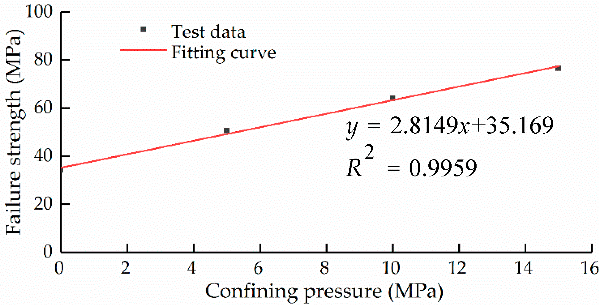
According to the triaxial compression test data of the surrounding rock, the mechanical parameters such as triaxial compression strength, modulus of elasticity, and Poisson’s ratio, were determined. When the influence of the confining pressure on the cohesion force and internal friction angle was not considered, the cohesion force and internal friction angle of surrounding rock could be determined by using data fitting according to the Mohr-Coulomb formula [13].
where c is the cohesion force of surrounding rock (MPa) and φ is the internal friction angle of surrounding rock (°).
The failure strength and fitting curve of the surrounding rock under different confining pressures are shown in Figure 2.
Thus, the elastic modulus, Poisson’s ratio, cohesion force, and internal friction angle of each specimen under triaxial condition were determined. The mechanical parameters of each test block are shown in Table 1.
3. Constitutive Model
From the curve of full stress versus strain, the surrounding rock in the subsea tunnel does not match the ideal elastoplastic model well. The biggest difference is that it has obvious softening characteristics after peak strength. Based on this, this section focuses on the post-peak softening law to establish the strain softening constitutive model of the surrounding rock.
Hardening and softening properties of rock depend on the hardening parameters which are the intrinsic factors affecting and controlling the deformation characteristics of rock [14]. In the process of strain hardening, the yield surface expands with the increase in the hardening parameter; in the process of strain softening, the yield surface shrinks with the decrease in the hardening parameter. Therefore, to study the strain softening constitutive model of rock, the hardening parameters must be determined first, and then the yield surface variation rule with hardening parameters is further determined. That is, the loading function of the rock has the following form:
where F is the loading function that controls the change in the subsequent yield and Hα are the hardening parameters.
The commonly used hardening parameters include plastic principal strain εip (I = 1, 2, 3), plastic shear strain γp, plastic volume strain εvp, and other plastic parameters. In the strain softening model of FLAC3D, the hardening parameter is called the plastic softening parameter, η. We assumed that the cohesion force c, the internal friction angle φ, and the dilatancy angle ψ are functions of plastic softening parameter η.
3.1. Evolution Law of Strength Parameters
This section mainly studies the evolution law of cohesion force c and the internal friction angle φ with the plastic softening parameter η, and the evolution law of the elastic modulus E and Poisson’s ratio μ with the confining pressure σ3.
The plastic softening parameter is determined as follows:
where ε1p, ε2p, ε3p are the first, second, and third plastic principal strains, respectively; ε1e, ε2e, ε3e are the first, second, and third elastic principal strains, respectively; ε1, ε2, ε3 are the first, second, and third total principal strains, respectively.
3.1.1. Evolution Law of c and φ with η
From Equations (5) to (9), the plastic softening parameters of rock under different confining pressures and different deviatoric stress can be determined. In the study, we considered that the rock was in the elastic stage before peak strength, and the main plastic strain produced before the peak strength was neglected, so the plastic softening parameter of peak strength was 0. The curve of relationship between post-peak deviatoric stress and post-peak plastic softening parameter is shown in Figure 3.
As shown in Figure 3, four groups of principal stresses—(σ11, σ31), (σ12, σ32), (σ13, σ33), and (σ14, σ34)—can be determined under the same plastic softening parameter. Then according to Equation (3), the cohesion force and the internal friction angles on the loading surface (for any plastic softening parameter) can be determined by using data fitting, which are shown in Figure 4. In order to depict the relationship between the cohesion force and plastic softening parameters, a fitting formula is proposed in Figure 4a. Also, in order to depict the relationship between the internal friction angles and plastic softening parameter, a fitting formula is proposed in Figure 4b.
3.1.2. Evolution Law of E and μ with σ3
According to the calculation results in Table 1, the elastic modulus and the Poisson’s ratios of rock under different confining pressures are determined and drawn in Figure 5. In order to depict the relationship between the elastic modulus and confining pressures, a fitting formula is proposed in Figure 5a. In order to depict the relationship between the Poisson’s ratios and confining pressures, a fitting formula is proposed in Figure 5b.
3.2. Evolution Law of Dilatancy Angle
According to the curve of the volume strain versus axial strain in Figure 1, the rate of change of the volume strain with the axial strain was constantly changing. The variation in the volume strain of rock is often represented by the dilatancy angle, and its calculation formula [15] is:
where Δεvp is plastic volume strain increment and Δε1p and Δε3p are plastic axial strain increment and plastic radial strain increment, respectively.
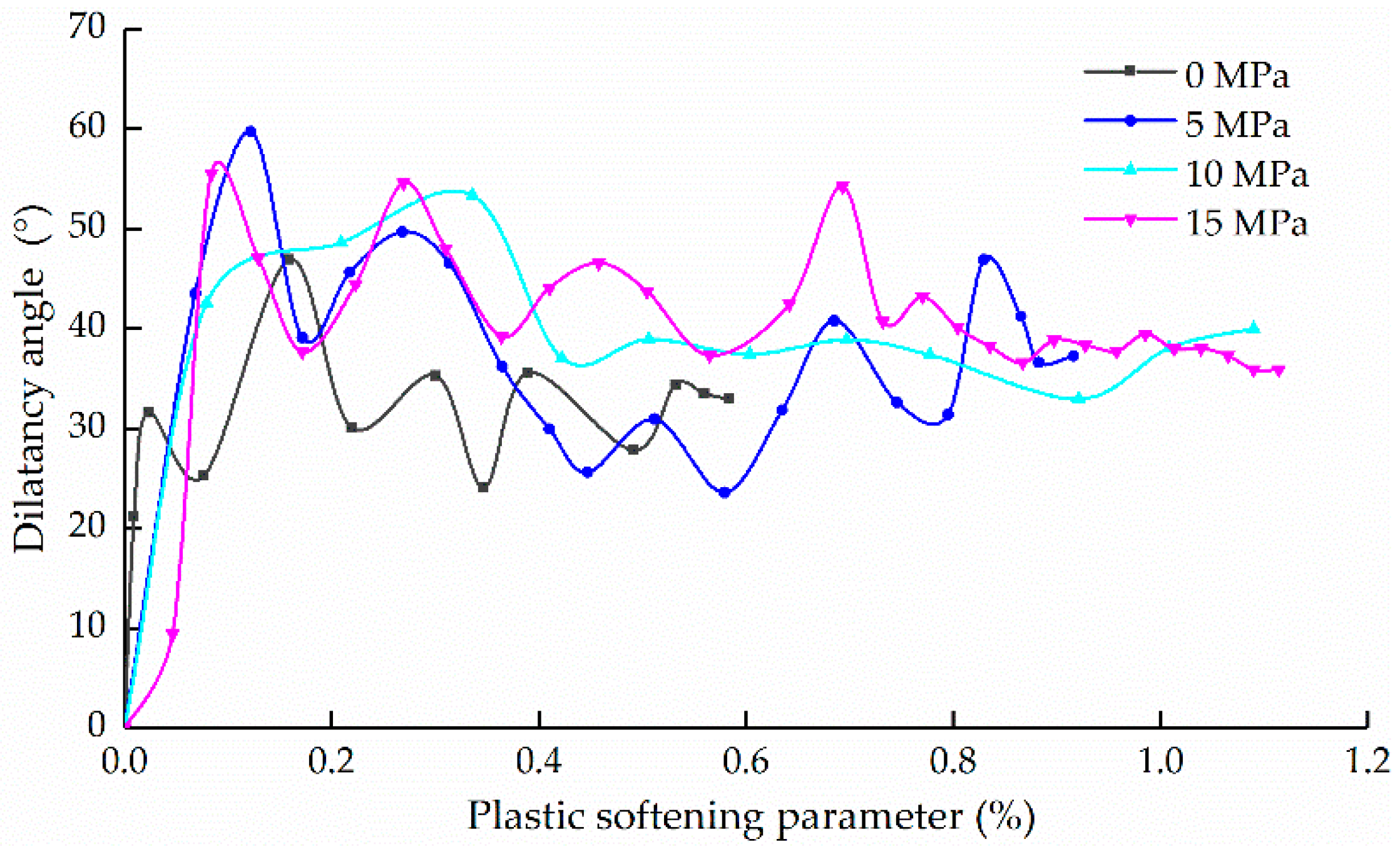
The dilatancy angles corresponding to different plastic softening parameters can be determined according to Equations (5)–(11). The negative dilatancy angle was ignored in the study (i.e., the dilatancy angle was 0 when the plastic softening parameter was 0). Therefore, we determined that the change law of the dilatancy angle with the plastic softening parameter under different confining pressures is as shown in Figure 6.
Through the study, we found that the relationship between dilatancy and plastic softening parameters under different confining pressures can be better fitted by using the following function.
where a, b and c are all fitting coefficients.
The fitting coefficients in Equation (12) under different confining pressures are given in Table 2.
By comparing the fitting coefficients a, b and c under different confining pressures in Table 2, it can be seen that the dilatancy angle was controlled not only by the plastic softening parameter, but also by the confining pressure, which cannot be ignored. In order to further determine the effect of confining pressure on the dilatancy angle, a function between the fitting coefficients a, b, c and confining pressure σ3 was established as follows.
The overall fitting of the relationship between confining pressure, plastic softening parameter and rock dilatancy angle can be determined by Equations (12)–(15). The comparison between the fitting curve and the measured value is shown in Figure 7.
The overall fitting curve of the dilatancy angle has a good corresponding relationship with the measured curve, which accurately reflects the stage characteristics of the sudden increase and steady decline of the dilatancy angle.
4. Evolution Law of Infiltration Characteristic and Numerical Verification
4.1. Evolution Law of Infiltration Characteristic
Fracture shape and width are two main reasons for the change in the permeability coefficient of rock. Although the relationship between permeability coefficient and the axial and radial strain is relatively difficult to establish, it is comparatively easy to establish a relationship between the permeability coefficient and the volume strain of rock. We assumed that the permeability coefficient of rock is controlled by the volume strain of rock. In addition, Zhao and Cai [15] considered that the change in volume strain of rock is controlled by the cohesion force, internal friction angle, Poisson’s ratio, and dilatancy angle of rock. Therefore, Section 2 and Section 3 are the basis for analyzing the evolution law of the permeability characteristics of rock.
Before the peak strength, the volume strain is usually greater than 0 (volume contraction) because no penetrating cracks are generated inside the rock. After the peak strength, the volume strain is usually less than 0 (volume inflation) due to the penetration of cracks, and the rock permeability coefficient increases dramatically. Therefore, according to the positive and negative volume strain, the evolution process of rock permeability is divided into two stages.
4.1.1. Case 1: εv > 0
According to the porous media elastic compression theory deduced by Li et al. [16], the formula for the change of permeability coefficient of rock at this stage is:
where K0 is the initial permeability coefficient (IPC), n0 is the initial porosity, p is the stress applied to the solid particle, Ks is the bulk modulus of the solid particle. In general, solid particles are difficult to compress, whose deformation can be negligible. Therefore, the formula for rock permeability when εv > 0 can be simplified as:
4.1.2. Case 2: εv < 0
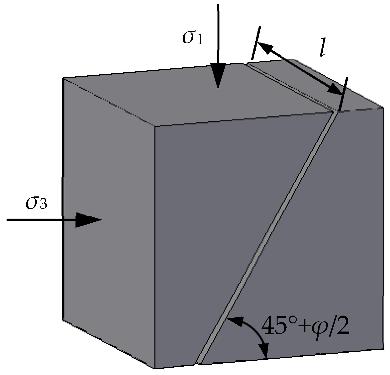
The phenomenon in the triaxial compression test showed that the rock failure is caused by the perforation of macroscopic fractures. Therefore, rock permeability depends almost entirely on the formation and morphology of the penetrating fractures. At present, the triaxial compression test of coupled stress-infiltration with a cylindrical specimen is usually used to study the evolution law of the rock permeability coefficient [17,18]. According to Mohr-Coulomb theory, the rock fracture angle (the angle between the rupture surface and the maximum principal stress direction) is about 45 + φ/2, and the internal friction angle is controlled by the confining pressure. Therefore, the crack opening e and the crack shape S are greatly affected by the shape of the specimen. In many cases, it is difficult to achieve complete penetration of the crack from the top surface to the bottom of the specimen and to analyze the nature of the evolution of the permeation performance.
According to the data from the triaxial compression test and Mohr theory [19], the internal friction angles of rock under different confining pressures can be obtained. The relationship between the internal friction angle and the confining pressure can also be obtained by data fitting.
In order to reveal the evolution law of infiltration of rock under loading conditions, a cubic element was used for analysis. The calculation model is shown in Figure 8. We assumed that the increase in rock volume was entirely due to a penetrating crevice, and that minor effects caused by changes in shape of the specimen were ignored.
According to Figure 8 and Equation (18), the crack opening is:
where e is the perforated crack opening (m), V0 is the initial volume of specimen (m3), S is the fracture surface area (m2), and l is the side length of the cube (m).
4.1.3. Analysis of Evolution Law of Infiltration Characteristic
Assume that the IPC of rock is 1.0 × 10⁻¹² m/s, the initial porosity is 0.01, the dynamic viscosity of water is 1.0 × 10⁻³ Pa·s, and the unit weight of fluid is 1.0 × 10⁴ N/m3. Based on the above theoretical calculations and the triaxial compression test data, the evolution curves of rock permeability coefficients under different confining pressures are shown in Figure 9.
The permeability coefficient of rock decreases continuously with the decrease in volume during the volume contraction stage (εv > 0), but the permeability coefficient of rock increases sharply with the increase in volume during volume inflation (εv < 0). In the volume inflation stage, the confining pressure has a certain influence on the permeability coefficient. The larger the confining pressure, the smaller the permeability coefficient, but the difference was not obvious. In practical applications, since the permeability coefficient of rock itself is very small, the change in the permeability coefficient in the volume contraction stage is completely negligible, and only the change in the permeability coefficient caused by volume inflation was considered.
4.2. Modeling and Verification of Triaxial Compression Test
4.2.1. Models and Parameters
Similar to the laboratory triaxial compression test, a cylindrical specimen (diameter d = 50.0 mm and height h = 100.0 mm) was used in the numerical simulation. The calculation model and the model specimen after the failure are shown in Figure 10. The tensile strength obtained from tensile strength test of rock was 2.328 MPa. Cohesion force and internal friction angle are depicted in Figure 4a,b respectively. The modulus of elasticity and Poisson’s ratio are depicted in Figure 5a,b respectively. The dilatancy angle is shown in Equations (12)–(15). The model lateral boundary was set to a constant pressure boundary, and the upper and lower boundaries were compressed inward at a constant rate. The strain softening model was used in the calculation and the relevant parameters were defined in the FISH language [23]. The parameters were updated in each calculation step to simulate the triaxial compression test process, and the model-related data were recorded.
4.2.2. Comparison of Results
According to the simulation results, the curves of the deviatoric stress versus axial strain, radial strain and volume strain versus axial strain of the test block were plotted. The simulation curve and test curve when the confining pressure was 10 MPa are shown in Figure 11.
From Figure 11, there is a good correspondence between the simulation curve and test curve, and the numerical simulation fully reflects the mechanical and deformation characteristics of the rock. Two reasons can explain the observed differences. (1) The calculation parameters were determined by fitting the data under different confining pressures, aiming at obtaining the fitting formulas of parameters that were used under different confining pressures, and not aiming at a specific confining pressure. Thus, when the data are highly discrete, it will inevitably cause a certain amount of error. (2) The specimen used in the triaxial compression test was essentially only one analysis unit, whereas the specimen in simulation consists of many units. Thus, the simulation curve reflects the reflection of the overall performance of many units, which inevitably led to the existence of errors.
4.2.3. Analysis of Evolution Law of Infiltration Characteristic
In the actual calculation, only the change in the rock permeability coefficient, which is determined by Equation (22), was considered when the volume strain was less than 0 (volume inflation). When the volume strain was greater than 0 (volume contraction), the rock permeability coefficient was completely negligible (i.e., the permeability coefficient of the volume contraction stage did not change). After the calculation of the model, the unit’s permeability coefficient was traversed and assigned by defining the unit extra variable.
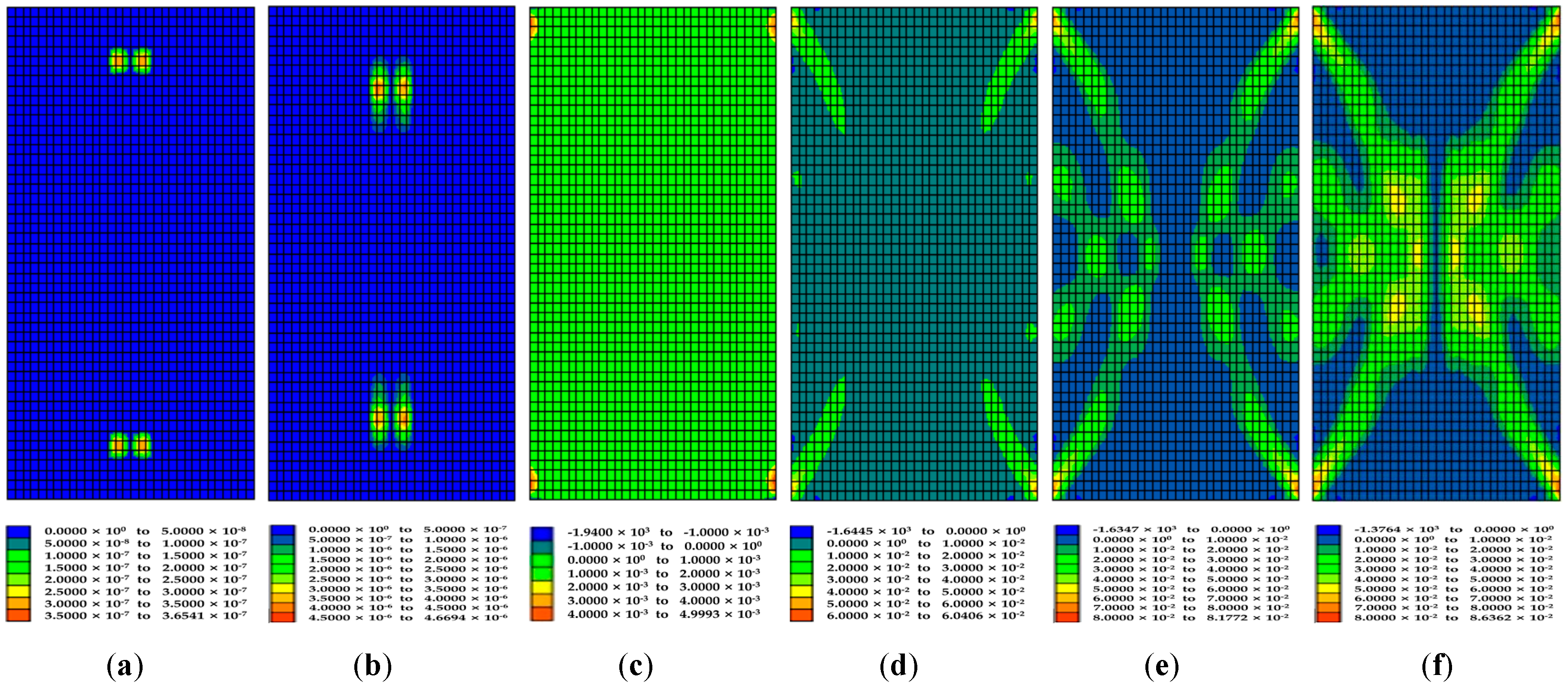
Figure 12 shows cloud pictures of the model specimen permeability coefficient distribution cross section at 400, 900, 1400, 1900, 2400, and 2900 steps. Among them, 400 and 900 steps are in front of the peak value of the deviator stress-axial strain curve, 1400 steps are positioned at the peak value, and 1900, 2400 and 2900 steps are behind the peak value.
It can be seen from Figure 12 that the model specimen permeability coefficient increased with calculation steps, and the figures gradually depict the fracture morphology. At 400 and 900 steps, the increase in the permeability coefficient was mainly concentrated in the middle micro area of the upper and lower parts of the specimen. From 1400 steps, the permeability coefficient of the specimen begins to be affected by the rupture surface, which significantly increases in the upper and lower edges of the specimen. At 2400 and 2900 steps, the specimen is completely fractured, the permeability coefficient increases significantly, and the fracture morphology is obvious.
5. Prediction of Water Inflow under Blasting Vibration
5.1. Models and Parameters
The studied subsea tunnel was excavated using the benching tunneling construction method. The circulating footage in the excavation was 2.0 m and the depth of the blast hole was 2.2 m. According to Guo et al. [24], it is possible to consider only the damage of the surrounding rock by the peripheral hole and ignore the superposition effect of the seismic wave. The blasting design parameters are shown in Table 3.
According to the reconnaissance report, the longitudinal wave velocity cpw of the surrounding rock was 3768.89 m/s and the shear wave velocity csw was 2083.33 m/s.
Since the excavation was carried out using the benching tunneling construction method in the actual project, in the study, the blasting calculations of the upper and lower sections were also carried out separately. In addition, in order to reflect the real boundary conditions, the scope of blasting simulation analysis was 15.0 m in front and 9.0 m behind the blasting range (2.0 m), totaling 26.0 m. According to the blasting design plan, there are 54 blast holes in the upper section and 28 blast holes in the lower section, totaling 82 blast holes as shown in Figure 13.
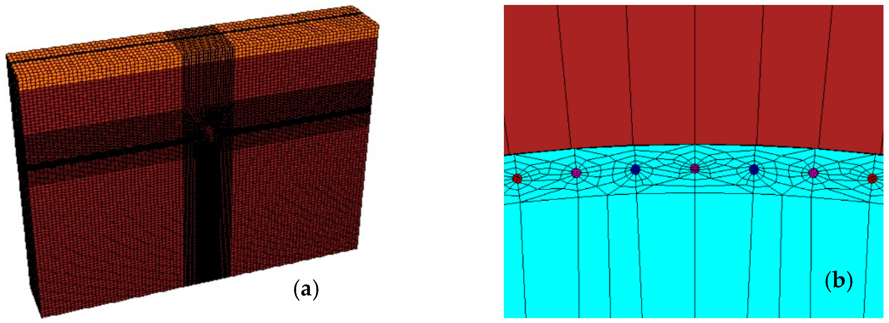
In order to make full use of the computational model and facilitate the subsequent comparative study, in the actual modeling, a blast hole was added to the middle of every two blast holes in the tunnel contour position. That is, there are 108 blast holes in the upper section and 57 blast holes in the lower section, totaling 165 simulated blast holes. Then water inflow was simulated after blasting simulation. Feng et al. [25] showed that accurate water inflow calculation results can be obtained when the distance from the left and right boundary to the tunnel lateral wall is greater than seven times the tunnel diameter, and the distance from the bottom boundary to the tunnel floor is also greater than seven times the tunnel diameter. Therefore, the calculated model length was 168 m and the height was 125.9 m. The corresponding calculation model is shown in Figure 14.
In order to shorten the calculation time, local damping was used to simulate, and the front, back, left, right and bottom boundaries of the whole model were set to static boundaries to reduce the reflection of the waves. In the blasting simulation, the most important thing was to accurately calculate the time history curve of the blasting load. Xin et al. [26] established the model of the blast hole and surrounding rock, and applied the blasting dynamic load to the boundary of the blast hole to determine the time history curve of the blasting dynamic load. According to the calculation of blasting parameters, the formula for calculating the time history curve of blasting load and the time history curve of the blasting load are shown in Figure 15, where P(t) is blasting load (MPa) and t is time (ms).
5.2. Mechanism Analysis of Surrounding Rock Permeability Increment under Blasting Vibration
The model calculation of the surrounding rock adopted the strain softening model established in Section 3. We considered that the increase in the surrounding rock permeability coefficient was mainly caused by the generation, development, and penetration of new cracks in the rock mass. After blasting vibration, the surrounding rock permeability coefficient was mainly composed of two parts: the IPC of the rock mass and the permeability coefficient increment of the rock mass under blasting vibration.
where Kb is the permeability coefficient of surrounding rock after blasting and K0 is the IPC of surrounding rock before blasting. Li et al. [27] proposed an approach to calculate the IPC by monitoring water inflow after tunnel excavation and using back analysis through numerical method. Finally, in this paper, after calculating the IPC, the K0 of surrounding rock was 0.0209 m/day and ΔK is the permeability coefficient increment in the rock mass after blasting.
Under blasting vibration, the surrounding rock is affected by the blasting load to produce internal damage and volume change. The evolution model of the surrounding rock permeability coefficient was used to determine permeability coefficient increment ΔK after surrounding rock blasting. Using the FISH language [23] and Equation (23) to re-traverse and assign the parameters for each unit, the distribution model of the surrounding rock permeability coefficient under blasting vibration was obtained. Since the permeability coefficient varied greatly after blasting, the visibility of the permeability coefficient distribution cloud map was poor. Therefore, the permeability coefficient increment distribution diagram of the surrounding rock was obtained by changing the value of the permeability coefficient increment as shown in Figure 16.
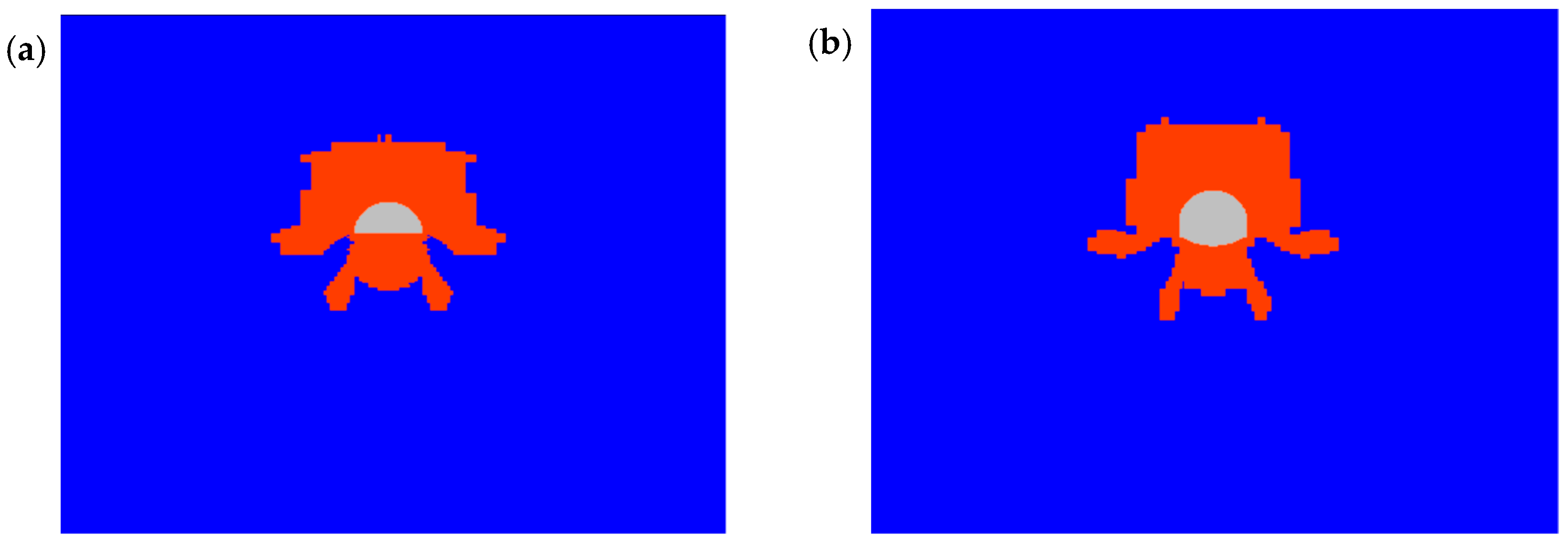
The zone of the permeability coefficient increment was mainly concentrated in the area around the excavation face. The influence of blasting on the surrounding area of the upper section of the tunnel was larger and more concentrated than around the lower section. The zone of permeability coefficient increment near the arch was the smallest and demonstrated obvious discontinuous characteristics. Since the upper section was arranged with the borehole at the bottom during the blasting process, the difference in the zone of permeability coefficient increment between the upper section and the full cross-section excavation was not obvious.
5.3. Prediction and Comparation of Water Inflow under Blasting Vibration
5.3.1. Field Test of Stable Water Inflow
The field test of stable water inflow of five blasting cycles in the 30 m excavation section was tested using the weir method. Due to the limitation of the construction site conditions, the stable water inflow was tested only after blasting for about 24 h. The test results are shown in Table 4.
5.3.2. Comparation and Analysis of Stable Water Inflow
FLAC3D was used to simulate the seepage field and water inflow in the subsea tunnel by using the exploration permeability coefficient (EPC) from the survey report and the IPC which was determined by water inflow after excavation. The permeability coefficient under blasting vibration (PCuBV) of the surrounding rock was used to analyze and calculate the seepage field and water inflow of the subsea tunnel under blasting vibration. In order to ensure the convergence of the calculation and accelerate the calculation speed, the permeability coefficient of each unit of the surrounding rock after blasting damage was extracted and imported into COMSOL multiphysics, which was no more than 10 cm/s. The distribution diagrams of seepage field of surrounding rock are shown in Figure 17.
The amount of water inflow in the subsea tunnel calculated by using the PCuBV was compared with the measured water inflow and the amount of water inflow calculated by using the EPC and the IPC of the surrounding rock. The calculation results and measured results are shown in Figure 18.
It can be seen from Figure 18 that the trend in water inflow in various situations of the subsea tunnel calculated over time was similar. The water inflow was larger in the initial stage of seepage, then decreased with time and tended to stabilize after about six hours. Since the assumption of a constant velocity was adopted in the calculation of water inflow after blasting vibration, and the variation of velocity with rock properties was neglected, only a single value was obtained, which corresponded to the final stationary state. As the blasting caused the permeability of the surrounding rock to increase, the stable water inflow quantity of the subsea tunnel under blasting vibration was larger than other working conditions. Comparing the measured water inflow in the upper section, the stable water inflow quantity from the upper section determined by EPC was 3.511 m3/day/m, which was much smaller than the measured water inflow of 4.6132 m3/day/m, and the stable water inflow quantity from the upper section determined by IPC was 4.318 m3/day/m, which was also smaller than the measured water inflow. Considering the blasting vibration, the water inflow was 4.764 m3/day/m, which was the closest to the measured value, but larger than the measured value, which may be because it was difficult to ensure that all the water outlets were tested in the field.
6. Conclusions
For the subsea tunnel of Qingdao metro line 1 in China, our goal was to predict the water flow into the subsea tunnel under blasting vibration. In this paper, a new practical approach to predict water inflow in subsea tunnel under blasting vibration was presented. The approach was developed by analyzing the mechanical and deformation characteristics of the surrounding rock through a laboratory triaxial compression test and then establishing the strain softening constitutive model of the surrounding rock. Based on the elastic compression theory of porous media and the cubic law of fractured rock mass, an evolution model of the permeability characteristics during the damage process of the surrounding rock was established. The evolution law of the permeability characteristics was analyzed.
In the calculation model during compression, the zone of the permeability coefficient increment increased, and a macro fracture gradually developed. The pre-peak infiltration area was small, and the post-peak infiltration area increased sharply. The post-peak infiltration area began to propagate from the edge of the upper and lower areas and then gradually penetrated the entire specimen.
In the calculation model under blasting vibration, the zone of the permeability coefficient increment was mainly concentrated in the area around the excavation face. The influence of blasting on the surrounding area of the upper section of the tunnel was larger and more concentrated than around the lower section. The zone of permeability coefficient increment near the arch was the smallest and demonstrated obvious discontinuous characteristics.
According to the actual blasting design scheme of the subsea tunnel, the surrounding rock constitutive model, and the permeability characteristic evolution model, the blasting process and water inflow of the subsea tunnel was simulated. The distribution of the surrounding rock permeability coefficient under blasting vibration was determined. Therefore, the water inflow quantity in subsea tunnels under blasting vibration was obtained. Water inflow quantity in the subsea tunnel under blasting vibration was compared with the water inflow quantity calculated using the EPC and the measured water inflow. We found that the predicted amount of water inflow under blasting vibration was closer to reality and more reasonable than existing models.
In conclusion, the workflow presented in this paper resulted in a valid and accurate approach for the prediction of water inflow under blasting vibration, since it considers the mechanical and deformation characteristics and the evolution law of inflation characteristics of surrounding rock.
Author Contributions
R.L. and D.X. conceived and designed the research; S.L. contributed ideas concerning the structure and content of the article; C.M. and C.Z. performed the experiments; R.L. and Y.L. analyzed the data and established the model; D.X., Z.Z. and Y.L. contributed to numerical simulation; C.Z. drew the figures. R.L. and Y.L. wrote the paper; Z.Z. reviewed and edited the manuscript.
Funding
This research was funded by Joint Funds of National Natural Science Foundation of China (U1706223), Shandong Provincial Natural Science Foundation (ZR201709230196), National Key R&D Plan of China (2016YFC0801604) and General Program of National Natural Science Foundation of China (51779133).
Acknowledgments
The authors would like to thank the Editors and anonymous Reviewers for their valuable and constructive comments related to this manuscript.
Conflicts of Interest
The authors declare no conflict of interest.
References
- Coli, N.; Pranzini, G.; Alifi, A.; Boerio, V. Evaluation of rock-mass permeability tensor and prediction of tunnel inflows by means of geostructural surveys and finite element seepage analysis. Eng. Geol. 2008, 101, 174–184. [Google Scholar] [CrossRef]
- Goodman, R.E.; Moye, D.G.; Schalkwyk, A.V.; Javandel, I. Ground water inflows during tunnel driving. Eng. Geol. 1965, 2, 39–56. [Google Scholar]
- Zhang, L.; Franklin, J.A. Prediction of water flow into rock tunnels: An analytical solution assuming a hydraulic conductivity gradient. Int. J. Rock Mech. Min. Sci. Geomech. Abstr. 1993, 30, 37–46. [Google Scholar] [CrossRef]
- Tani, M.E. Circular tunnel in a semi-infinite aquifer. Tunn. Undergr. Space Technol. Inc. Trenchless Technol. Res. 2003, 18, 49–55. [Google Scholar] [CrossRef]
- Park, K.H.; Owatsiriwong, A.; Lee, J.G. Analytical solution for steady-state groundwater inflow into a drained circular tunnel in a semi-infinite aquifer: A revisit. Tunn. Undergr. Space Technol. Inc. Trenchless Technol. Res. 2008, 23, 206–209. [Google Scholar]
- Perrochet, P. A simple solution to tunnel or well discharge under constant drawdown. Hydrogeol. J. 2005, 13, 886–888. [Google Scholar] [CrossRef]
- Renard, P. Approximate discharge for constant head test with recharging boundary. Groundwater 2010, 43, 439–442. [Google Scholar] [CrossRef] [PubMed]
- Ainalis, D.; Kaufmann, O.; Tshibangu, J.P.; Verlinden, O.; Kouroussis, G. Modelling the source of blasting for the numerical simulation of blast-induced ground vibrations: A review. Rock Mech. Rock Eng. 2016, 50, 171–193. [Google Scholar] [CrossRef]
- Rutqvist, J.; Börgesson, L.; Chijimatsu, M.; Hernelind, J.; Jing, L.; Kobayashi, A.; Nguyen, S. Modeling of damage, permeability changes and pressure responses during excavation of the TSX tunnel in granitic rock at URL, Canada. Environ. Geol. 2009, 57, 1263–1274. [Google Scholar] [CrossRef]
- Hao, H.; Wu, C.; Zhou, Y. Numerical analysis of blast-induced stress waves in a rock mass with anisotropic continuum damage models part 1: Equivalent material property approach. Rock Mech. Rock Eng. 2002, 35, 79–94. [Google Scholar] [CrossRef]
- Wu, C.; Lu, Y.; Hao, H. Numerical prediction of blast-induced stress wave from large-scale underground explosion. Int. J. Numer. Anal. Methods Geomech. 2004, 28, 93–109. [Google Scholar] [CrossRef]
- Bäckblom, G.; Martin, C.D. Recent experiments in hard rocks to study the excavation response: Implications for the performance of a nuclear waste geological repository. Tunn. Undergr. Space Technol. 1999, 14, 377–394. [Google Scholar] [CrossRef]
- Zhao, J. Applicability of Mohr-Coulomb and Hoek-Brown strength criteria to the dynamic strength of brittle rock. Int. J. Rock Mech. Min. Sci. 2000, 37, 1115–1121. [Google Scholar] [CrossRef]
- Zheng, Y.R.; Kong, L. Geotechnical Plastic Mechanics, 1st ed.; China Architecture & Building Press: Beijing, China, 2010; pp. 143–154. ISBN 978-7-12-11668-3. [Google Scholar]
- Zhao, X.; Cai, M. A rock dilation angle model and its verification. Chin. J. Rock Mech. Eng. 2010, 29, 970–981. [Google Scholar]
- Li, P.C.; Kong, X.Y.; De-Tang, L.U. Mathematical modeling of flow in saturated porous media on account of fluid-structure coupling effect. J. Hydrodyn. 2003, 18, 419–426. [Google Scholar]
- Yu, J.; Li, H.; Chen, X.; Cai, Y.; Wu, N.; Mu, K. Triaxial experimental study of associated permeability-deformation of sandstone under hydro-mechanical coupling. Chin. J. Rock Mech. Eng. 2013, 32, 1203–1213. [Google Scholar]
- Hu, S.; Chen, Y.; Zhou, C. Laboratory test and mesomechanical analysis of permeability variation of beishan granite. Chin. J. Rock Mech. Eng. 2014, 33, 2200–2209. [Google Scholar]
- Cai, M.F. Rock Mechanics and Engineering, 2nd ed.; Science Press: Wuhan, China, 2013; pp. 214–216. ISBN 703010470. [Google Scholar]
- Dreuzy, J.R.D.; Davy, P.; Bour, O. Hydraulic properties of two-dimensional random fracture networks following power law distributions of length and aperture. Water Resour. Res. 2002, 38. [Google Scholar] [CrossRef]
- Klimczak, C.; Schultz, R.A.; Parashar, R.; Reeves, D.M. Cubic law with aperture-length correlation: Implications for network scale fluid flow. Hydrogeol. J. 2010, 18, 851–862. [Google Scholar] [CrossRef]
- Swartzendruber, D. Darcy’s law. Encyclopedia Soils Environ. 2005, 24, 363–369. [Google Scholar]
- Jay, C.B. The FISH Language Definition; Technical Report; School of Computing Sciences, University of Technology: Sydney, Australia, 1998. [Google Scholar]
- Guo, Y.J.; Bang-Shu, X.U.; Song, Z.Q. Study on induced-blasting damage of covering rocks in submarine tunnel construction. J. Shandong Univ. Sci. Technol. 2008, 27, 56–62. [Google Scholar]
- Feng, X.D.; Shu-Chen, L.I.; Bang-Shu, X.U. Numerical simulation study on influence factors of the seepage volume of submarine tunnels. J. Shandong Univ. 2009, 39, 21–24. [Google Scholar]
- Xin, Z.; Shucai, L.I. Stability analysis of rock cover of Qingdao Kiaochow bay subsea tunnel under explosive loads. Chin. J. Rock Mech. Eng. 2007, 26, 2348–2355. [Google Scholar]
- Li, L.C.; Tang, C.A.; Liang, Z.Z.; Ma, T.H.; Zhang, Y.B. Numerical simulation on water inrush process due to activation of collapse columns in coal seam floor. J. Min. Saf. Eng. 2009, 26, 158–162. [Google Scholar]
Figure 1.
Triaxial compression test curves of (a) deviatoric stress vs. axial strain and radial strain and (b) volume strain vs. axial strain.
Figure 1.
Triaxial compression test curves of (a) deviatoric stress vs. axial strain and radial strain and (b) volume strain vs. axial strain.
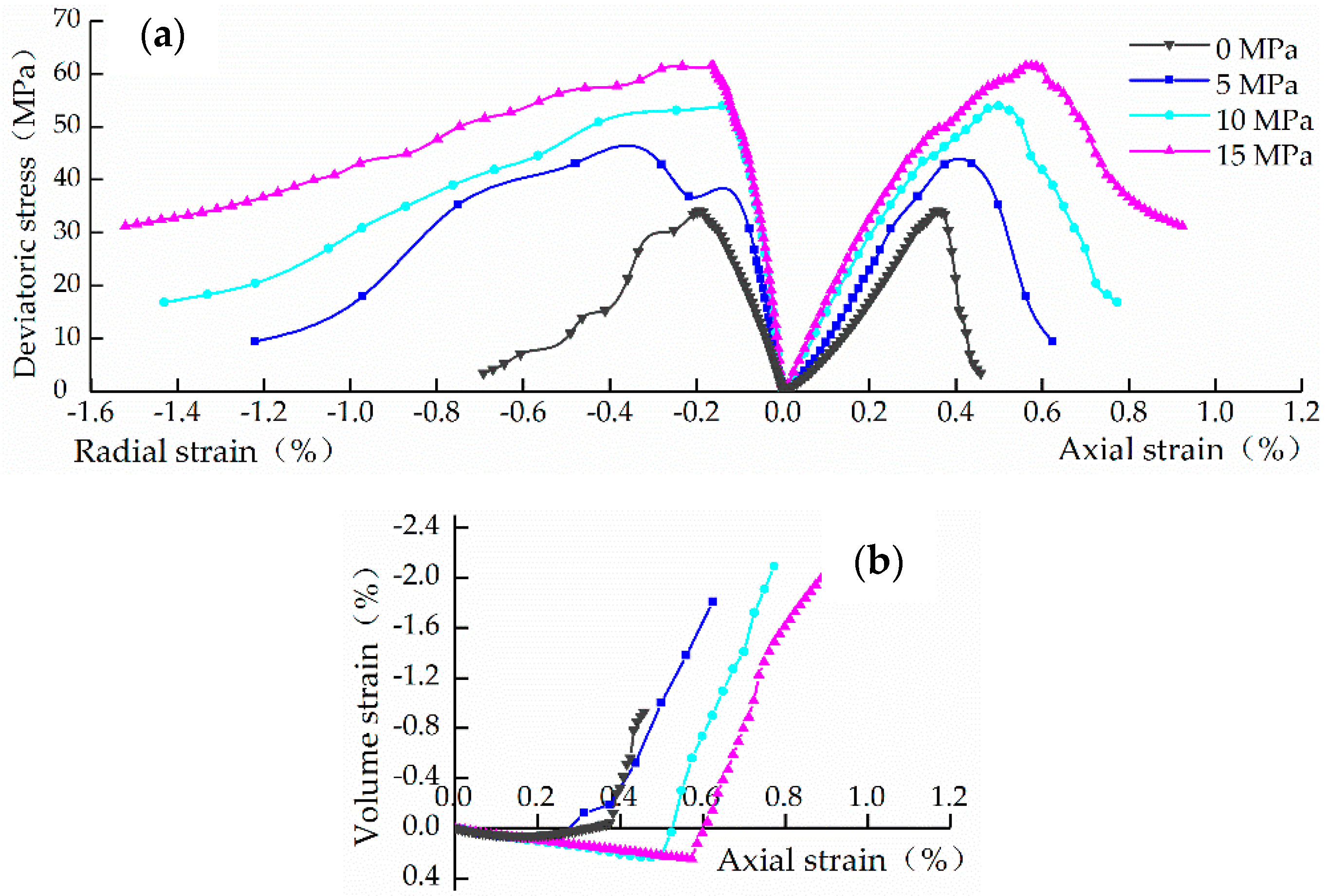
Figure 2.
Failure strength and fitting curve under different confining pressures.

Figure 3.
Relationship between post-peak deviatoric stress and plastic softening parameter.
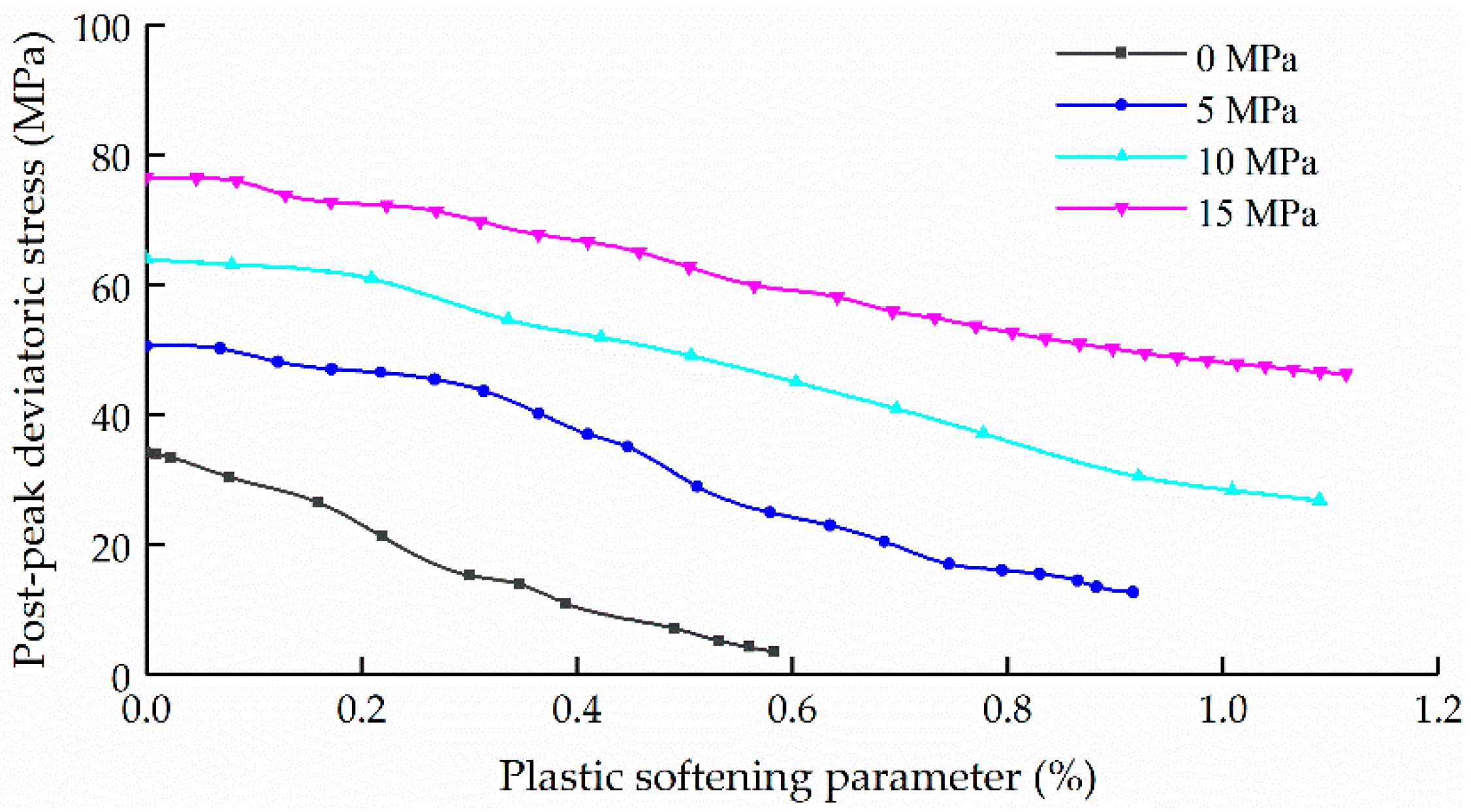
Figure 4.
Regression curves of (a) cohesion force vs. plastic softening parameter and (b) internal friction angle vs. plastic softening parameter.
Figure 4.
Regression curves of (a) cohesion force vs. plastic softening parameter and (b) internal friction angle vs. plastic softening parameter.
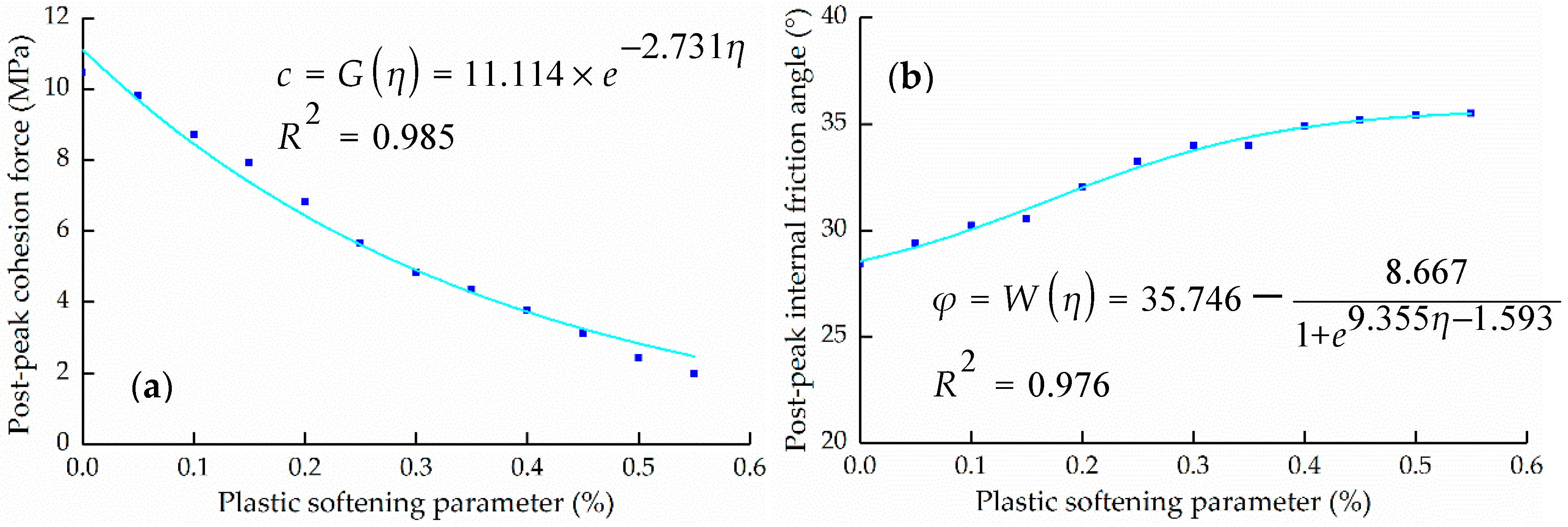
Figure 5.
Regression curves of (a) elastic modulus vs. confining pressure and (b) Poisson’s ratios vs. confining pressure.
Figure 5.
Regression curves of (a) elastic modulus vs. confining pressure and (b) Poisson’s ratios vs. confining pressure.
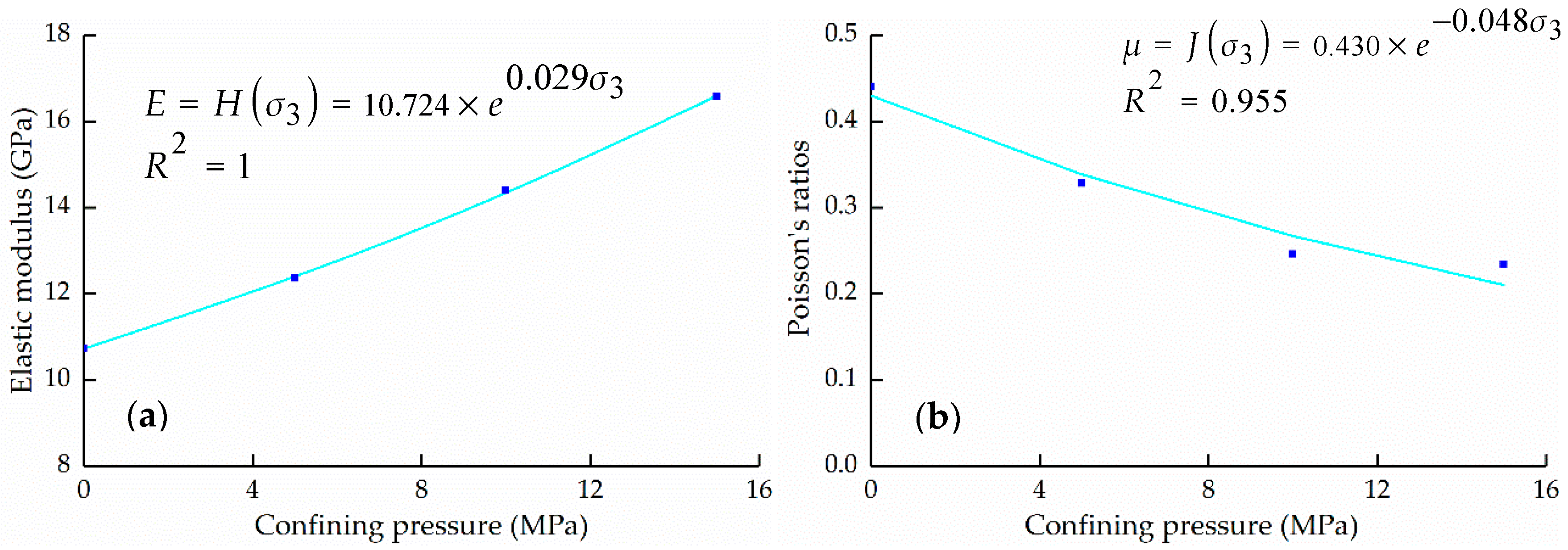
Figure 6.
Dilatancy angle vs. the plastic softening parameter under different confining pressures.

Figure 7.
The fitting curve of the dilatancy angle.
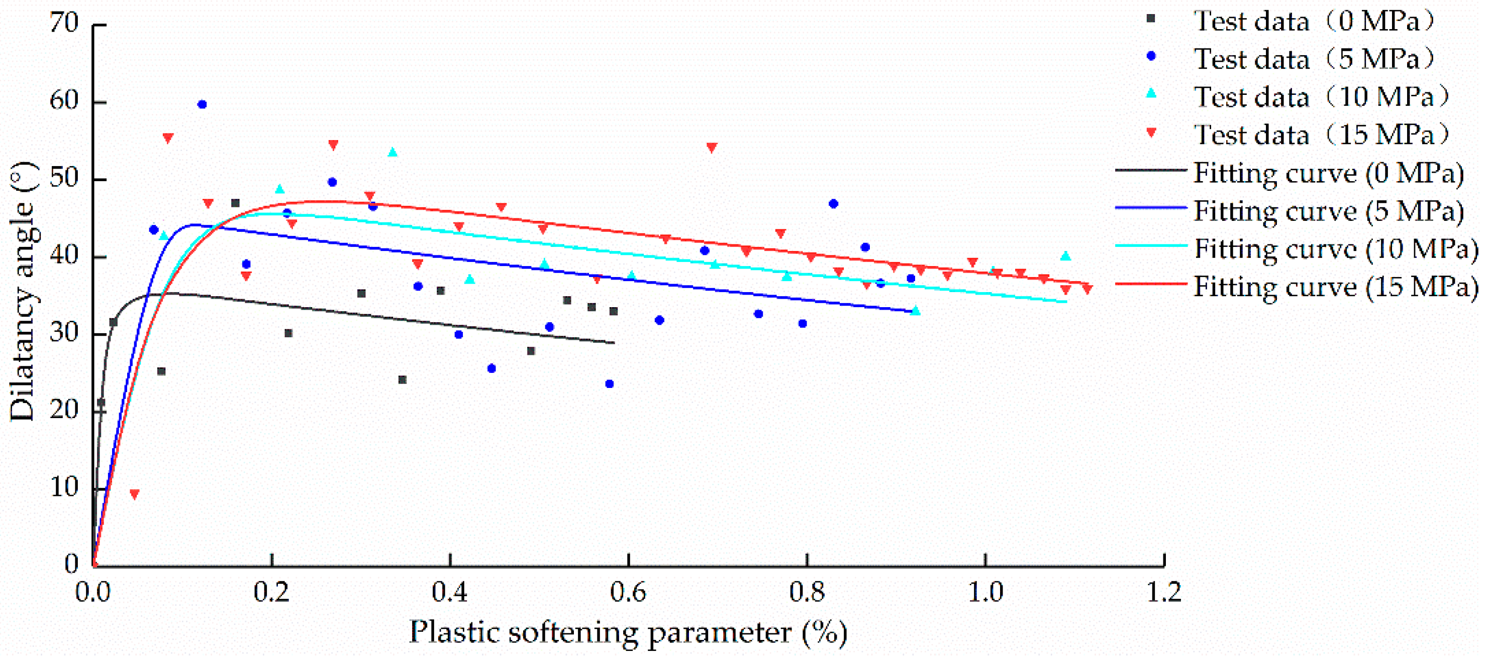
Figure 8.
Calculation model diagram.

Figure 9.
The evolution curves of infiltration characteristic. (a) Case 1: εv > 0; (b) Case 2: εv < 0.
Figure 9.
The evolution curves of infiltration characteristic. (a) Case 1: εv > 0; (b) Case 2: εv < 0.

Figure 10.
The calculation model and the model after failure.
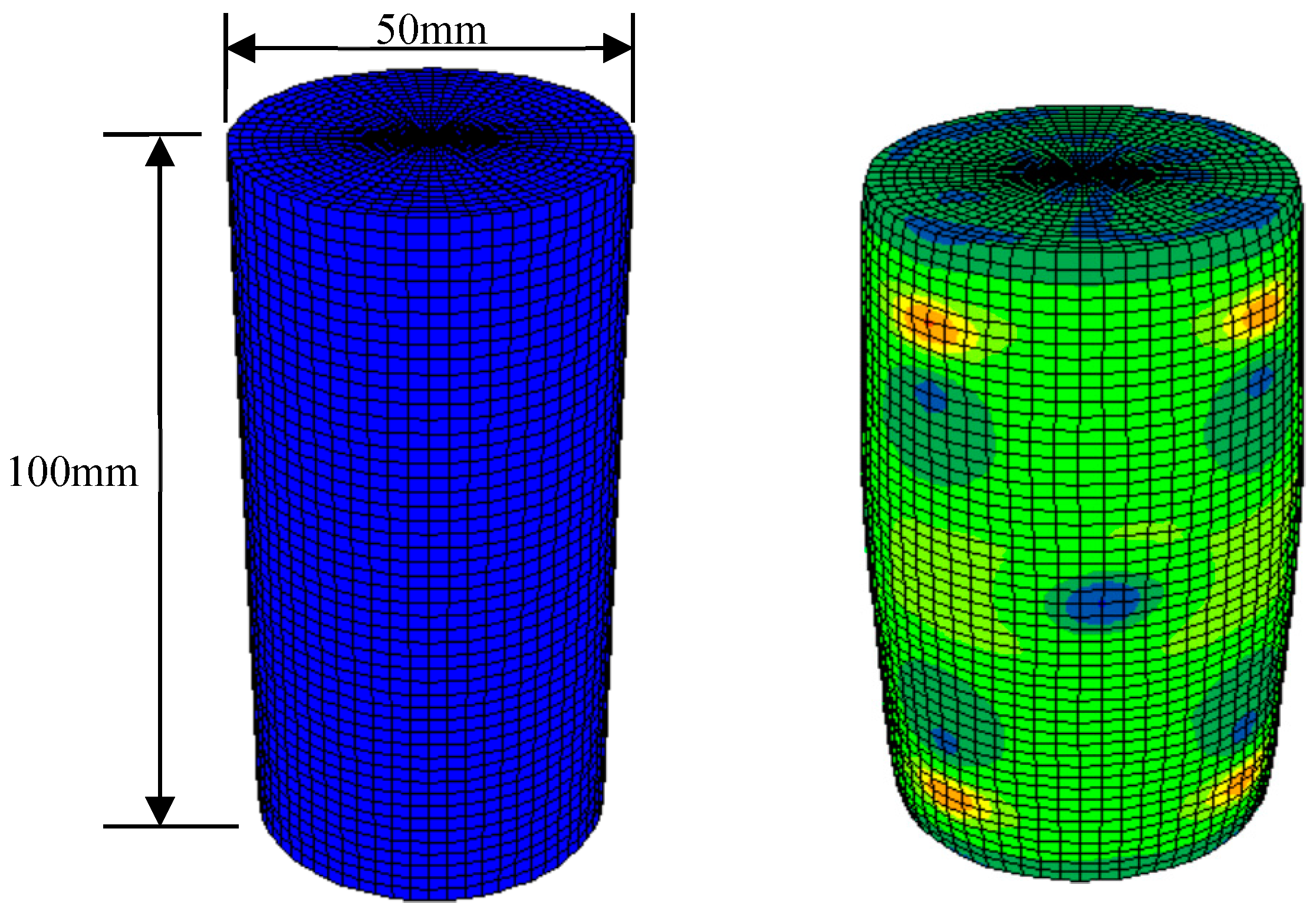
Figure 11.
The simulation curve and test curve of (a) deviatoric stress vs. axial strain and radial strain and (b) volume strain vs. axial strain when the confining pressure is 10 MPa.
Figure 11.
The simulation curve and test curve of (a) deviatoric stress vs. axial strain and radial strain and (b) volume strain vs. axial strain when the confining pressure is 10 MPa.
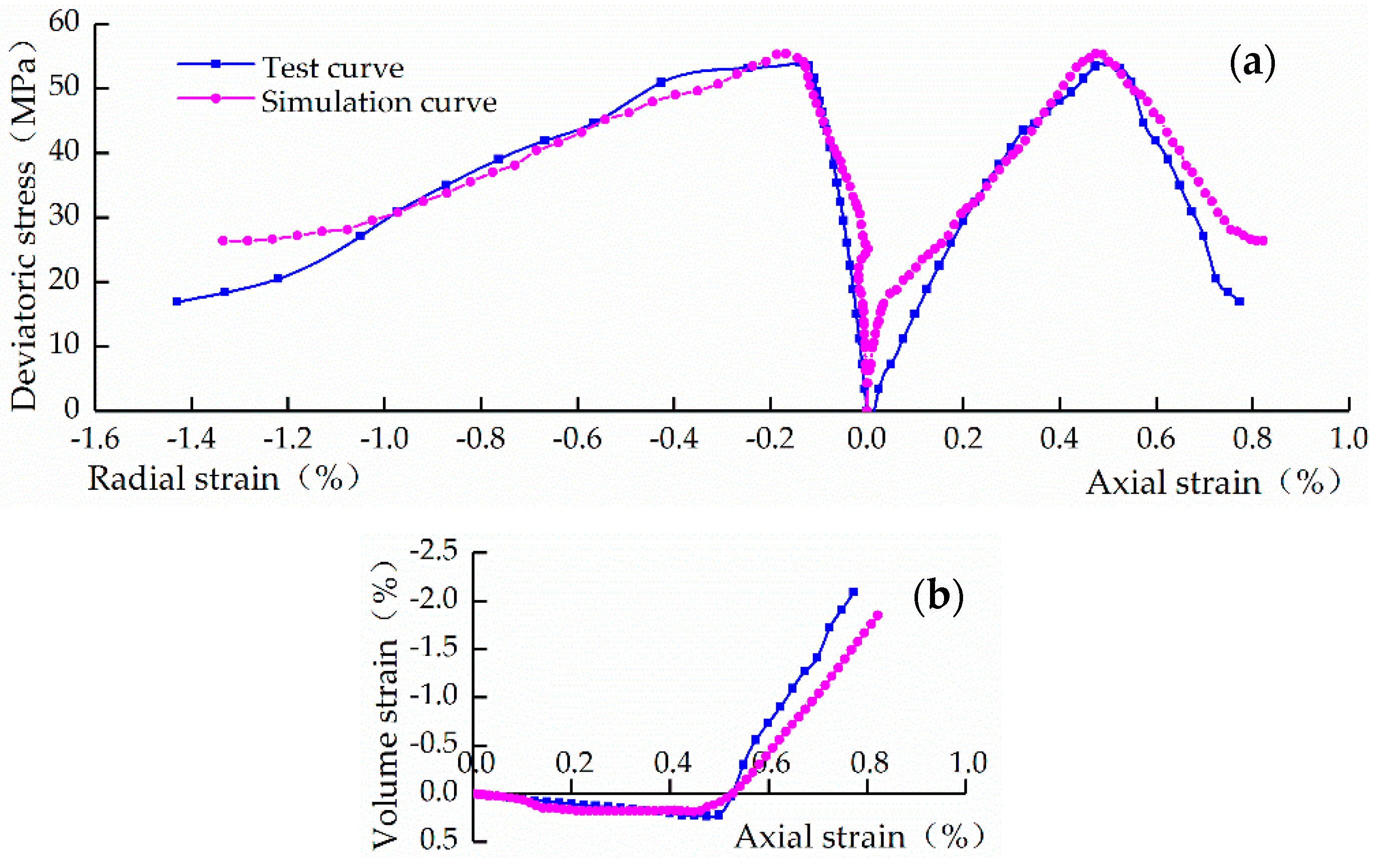
Figure 12.
Cloud pictures of the permeability coefficient distribution of model specimen cross section at (a) 400, (b) 900, (c) 1400, (d) 1900, (e) 2400, and (f) 2900 steps.
Figure 12.
Cloud pictures of the permeability coefficient distribution of model specimen cross section at (a) 400, (b) 900, (c) 1400, (d) 1900, (e) 2400, and (f) 2900 steps.

Figure 13.
Layout drawing of blast holes.

Figure 14.
Computational model diagram. (a) Overall module. (b) Enlarged view of vault hole.

Figure 15.
The time history curve of blasting load.

Figure 16.
Permeability coefficient increment distribution diagram of surrounding the rock after blasting. (a) upper section. (b) full cross-section.
Figure 16.
Permeability coefficient increment distribution diagram of surrounding the rock after blasting. (a) upper section. (b) full cross-section.

Figure 17.
The distribution diagrams of seepage field of surrounding rock calculated by using (a) exploration permeability coefficient (EPC), (b) initial permeability (IPC), (c) permeability coefficient under blasting vibration (PCuBV).
Figure 17.
The distribution diagrams of seepage field of surrounding rock calculated by using (a) exploration permeability coefficient (EPC), (b) initial permeability (IPC), (c) permeability coefficient under blasting vibration (PCuBV).

Figure 18.
The compared diagrams of water inflow in the subsea tunnel. (a) upper section and (b) full-cross section.
Figure 18.
The compared diagrams of water inflow in the subsea tunnel. (a) upper section and (b) full-cross section.


Table 1.
Mechanical parameters obtained from the triaxial test.
| Number | Confining Pressure (σ3/MPa) | Peak Deviatoric Stress (q/MPa) | Compressive Strength (σc/MPa) | Elasticity Modulus (E/GPa) | Poisson’s Ratio (μ) | Cohesion Force (c/MPa) | Internal Friction Angle (φ/°) |
|---|---|---|---|---|---|---|---|
| 1–1 | 0 | 34.077 | 34.077 | 10.447 | 0.479 | 10.481 | 28.408 |
| 1–2 | 0 | 36.126 | 36.126 | 11.029 | 0.383 | ||
| 2–1 | 5.0 | 45.564 | 50.564 | 12.349 | 0.330 | ||
| 2–2 | 5.0 | 46.272 | 51.272 | 12.364 | 0.325 | ||
| 3–1 | 10.0 | 54.553 | 64.553 | 13.892 | 0.257 | ||
| 3–2 | 10.0 | 53.950 | 63.950 | 14.910 | 0.234 | ||
| 4–1 | 15.0 | 61.348 | 76.348 | 16.337 | 0.226 | ||
| 4–2 | 15.0 | 61.531 | 76.531 | 16.811 | 0.242 |
Table 2.
Fitting coefficients for Equation (12) under different confining pressures.
| Confining Pressure σ3/MPa | a | b | c |
|---|---|---|---|
| 0 | 36.741 | 119.553 | 0.417 |
| 5 | 45.933 | 63.177 | 0.367 |
| 10 | 49.020 | 33.671 | 0.339 |
| 15 | 51.220 | 15.881 | 0.321 |
Table 3.
Blasting parameters.
| Circulating Footage (lk/m) | Detonation Speed (vb/km/s) | Radius of Stick Dynamite (rc/m) | Radius of Borehole (rd/m) | Charge Density (ρ°/g/cm3) |
|---|---|---|---|---|
| 2.0 | 4.5 | 0.016 | 0.02 | 1.0 |
Table 4.
Results of water inflow of upper section.
| Blasting Cycles | 2 | 5 | 8 | 11 | 14 | Mean Value |
|---|---|---|---|---|---|---|
| Inflow water/(m3/day/m) | 2.551 | 13.415 | 5.140 | 0.000 | 1.960 | 4.613 |
© 2018 by the authors. Licensee MDPI, Basel, Switzerland. This article is an open access article distributed under the terms and conditions of the Creative Commons Attribution (CC BY) license (http://creativecommons.org/licenses/by/4.0/).
Share and Cite
MDPI and ACS Style
Liu, R.; Liu, Y.; Xin, D.; Li, S.; Zheng, Z.; Ma, C.; Zhang, C. Prediction of Water Inflow in Subsea Tunnels under Blasting Vibration. Water 2018, 10, 1336. https://doi.org/10.3390/w10101336
AMA Style
Liu R, Liu Y, Xin D, Li S, Zheng Z, Ma C, Zhang C. Prediction of Water Inflow in Subsea Tunnels under Blasting Vibration. Water. 2018; 10(10):1336. https://doi.org/10.3390/w10101336
Chicago/Turabian StyleLiu, Rentai, Yankai Liu, Dongdong Xin, Shucai Li, Zhuo Zheng, Chenyang Ma, and Chunyu Zhang. 2018. "Prediction of Water Inflow in Subsea Tunnels under Blasting Vibration" Water 10, no. 10: 1336. https://doi.org/10.3390/w10101336
Note that from the first issue of 2016, this journal uses article numbers instead of page numbers. See further details here.