Rainfall-Runoff Modelling Considerations to Predict Streamflow Characteristics in Ungauged Catchments and under Climate Change


CSIRO Land and Water, Black Mountain, Canberra ACT 2601, Australia
*
Author to whom correspondence should be addressed.
Water 2018, 10(10), 1319; https://doi.org/10.3390/w10101319
Submission received: 30 May 2018
/
Revised: 19 September 2018
/
Accepted: 21 September 2018
/
Published: 24 September 2018
(This article belongs to the Special Issue Enhancing Hydrological Prediction through Modelling with Large Datasets)
Abstract
:This paper investigates the prediction of different streamflow characteristics in ungauged catchments and under climate change, with three rainfall-runoff models calibrated against three different objective criteria, using a large data set from 780 catchments across Australia. The results indicate that medium and high flows are relatively easier to predict, suggesting that using a single unique set of parameter values from model calibration against an objective criterion like the Nash–Sutcliffe efficiency is generally adequate and desirable to provide a consistent simulation and interpretation of daily streamflow series and the different medium and high flow characteristics. However, the low flow characteristics are considerably more difficult to predict and will require careful modelling consideration to specifically target the low flow characteristic of interest. The modelling results also show that different rainfall-runoff models and different calibration approaches can give significantly different predictions of climate change impact on streamflow characteristics, particularly for characteristics beyond the long-term averages. Predicting the hydrological impact from climate change, therefore, requires careful modelling consideration and calibration against appropriate objective criteria that specifically target the streamflow characteristic that is being assessed.
1. Introduction
Hydrological models are widely used for water resources assessment, to estimate water availability and describe streamflow characteristics important for many applications, and to predict how these may change in the future [1,2]. The key challenges in hydrological modelling include conceptualising the dominant processes [1], calibrating and validating the models against streamflow and other observations [2], and predicting the future under development drivers and land-use and climate change [3,4]. The main traditional approach is to calibrate and validate the hydrological models to reproduce the observed streamflow and sometimes other variables like soil moisture or remotely sensed evapotranspiration and snow cover [5,6]. To predict streamflow in ungauged areas, approaches include using parameter values from a physically similar gauged catchment, using calibrated parameter values from the geographically closest gauged catchment, or regionally calibrating to obtain a single parameter set for an entire region that best reproduces the overall observed flows at all gauged sites within the region [2,7,8,9].
Hydrological models are generally calibrated against an objective function or criteria, like the root mean squared error (RMSE), Nash–Sutcliffe efficiency (NSE) [10] or Kling–Gupta efficiency (KGE) [11], that minimise the difference between the modelled and observed streamflow series. However, calibrating a model against an objective function that targets a particular flow characteristic may perform sub-optimally in reproducing other flow characteristics. Therefore, a trade-off is usually required in selecting an objective function if a single set of parameter values is to be used to consistently model the entire streamflow series and the different flow characteristics. The alternative is to calibrate the model against an objective function that specifically targets the flow characteristic of interest (e.g., low flows [12], or floods and high flows [13,14]) and accepting poorer simulation of other flow characteristics.
This paper explores the above considerations using three lumped conceptual daily rainfall-runoff models applied to a large data set across Australia. Specifically, the paper investigates the ability of the models calibrated against three different objective functions, which reflect or target daily flow simulation, high flow simulation and low flow simulation, to simulate streamflow characteristics like mean annual streamflow, daily streamflow time series, high flow and low flow. These are assessed for three applications: (i) model simulation in single catchments; (ii) prediction in ungauged catchments; and (iii) modelling climate change impact on streamflow characteristics.
The motivation of the paper is to investigate the following questions of interest relating to practical applications:
- Do we need a different calibration objective function or criteria to target each specific streamflow characteristic or signature? or
- Is there a general calibration criteria that can adequately reproduce most streamflow characteristics? (Hence allowing for a consistent simulation of streamflow time series and the different streamflow characteristics using one single set of parameter values); or
- Do we need a couple of calibration criteria for groups of similar types of streamflow characteristics? and
- What are the implications when the calibrated model is then used to predict changes in the different flow characteristics under climate change?
We are not aware of papers in the literature that address these questions collectively. Nevertheless, the broad results from the various components of this study are largely similar to those reported in previous studies, and these are presented and stated in the paper. The paper then explores the above questions in some detail, and the modelling with the large dataset across the large range of hydroclimates in Australia here allows some generalisation of the results.
The data and methods are described in Section 2, with the above three applications described in separate subsections. The results are presented in Section 3, also with the same subsections for the three applications. Reading the related subsections together (e.g., Section 2.1 and Section 3.1, Section 2.2 and Section 3.2, Section 2.3 and Section 3.3) may facilitate better understanding and interpretation of the methods and results. The results and implications are then discussed in Section 4, with summary and conclusions in Section 5.
2. Data and Methods
The modelling is carried out with three commonly used lumped conceptual daily rainfall-runoff models: GR4J [15], SIMHYD [16] and Xinanjiang [17]. All three models conceptualise the catchment as consisting of several storages representing vegetation, soil moisture and/or groundwater, with mathematical equations describing the movement of water into and out of the stores. The input data are daily rainfall and potential evapotranspiration, and the model simulates daily streamflow. The GR4J model is based on unit hydrograph principles. It has four parameters, with the model developers showing that the use of four parameters was optimum or most parsimonious from model testing against an extensive dataset across the world. The GR4J model allows water to enter or leave the catchment. In contrast, the SIMHYD and Xinanjiang models are closed water balance models, where long term precipitation is equal to long term actual evapotranspiration plus runoff. The SIMHYD model is a simple lumped conceptual rainfall-runoff model commonly used in Australia, and the model version used here has five parameters. The Xinanjiang model has been used for many applications globally, and the model version used here has 13 parameters. The Xinanjiang model explicitly simulates a partial area runoff generation process through conceptualising the catchment storage capacity using a parabolic relationship.
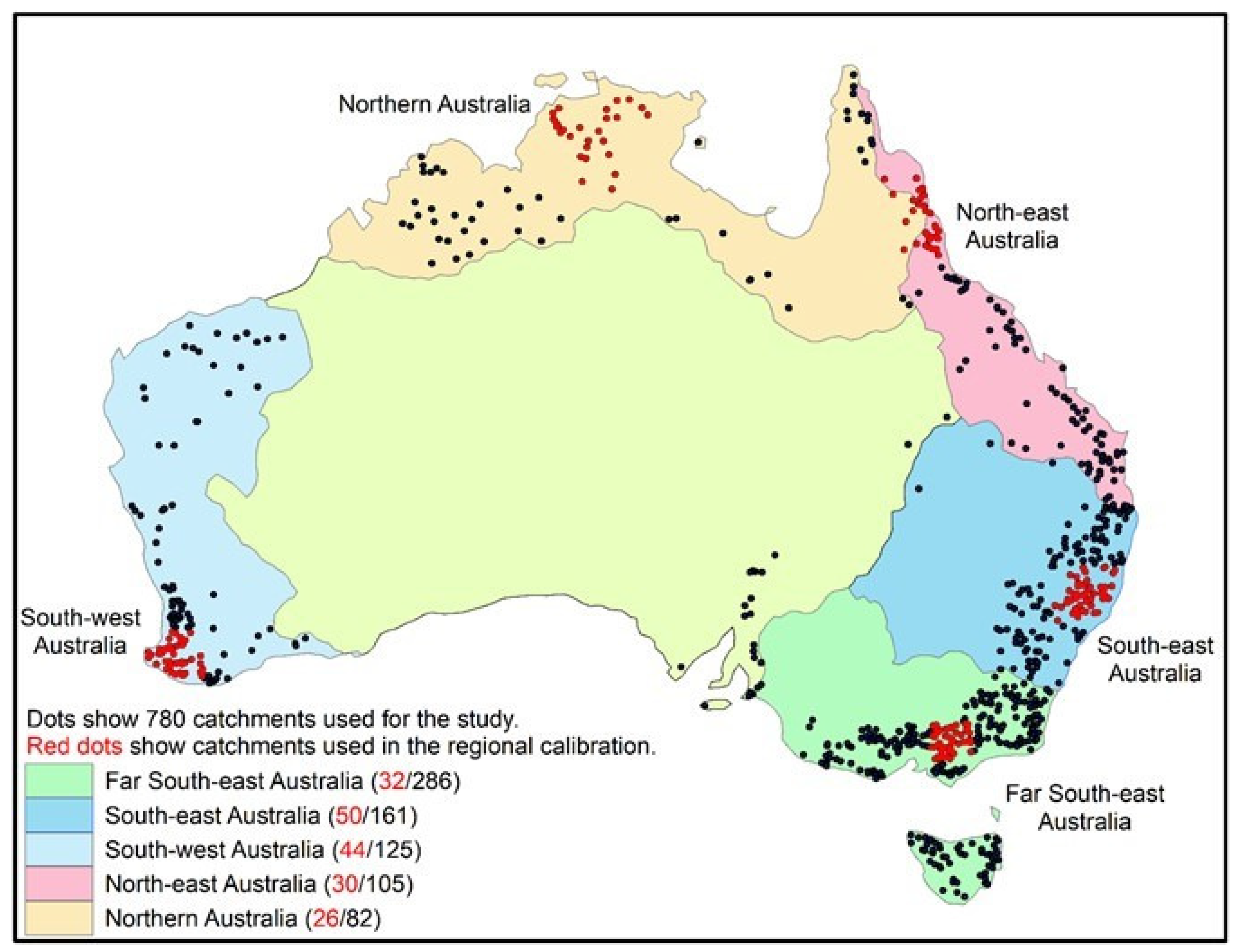
The modelling is carried out using data from 780 catchments across Australia. Figure 1 shows the locations of the catchments and Table 1 summarises the catchment characteristics. Thirty years of daily rainfall, potential evapotranspiration and streamflow data from 1981 to 2010 are used for the modelling. The rainfall and climate data come the SILO Data Drill (https://legacy.longpaddock.qld.gov.au/silo/datadrill/ [18]), which provides surfaces of daily climate data for 0.05° (~5 km) grids across Australia, interpolated from point measurements from the Australian Bureau of Meteorology data set. The potential evapotranspiration is calculated from the SILO climate surface using Morton’s wet environment or areal potential evapotranspiration algorithm [19,20]. The modelling here uses lumped catchment daily rainfall and potential evapotranspiration series obtained by aggregating/averaging the data from the grid cells contributing to the catchment.
The streamflow data for the 780 catchments come from the state and territory water agencies and the Bureau of Meteorology and has been compiled and curated for quality [21]. Most of the catchments have practically complete continuous daily streamflow data over the 30-year 1981–2010 period, and none of the catchments have more than 5% missing streamflow data. All the catchments are largely unimpaired (i.e., no river regulation and little land-use change over the modelling period), with catchment areas ranging from 100 km2 to 3000 km2 (10th and 90th percentile range). As can been seen in Figure 1, apart from the arid interior (where there is very little data), the catchments cover all parts of Australia particularly the populated and important agricultural region in the south-east.
The models are calibrated separately against three objective criteria: NSE-Daily-Bias; NSE-High; and NSE-Low.
The NSE-Daily-Bias criteria [22] is defined as,
where,
where, is modelled daily streamflow, is observed daily streamflow, is mean modelled streamflow, is mean observed streamflow, and n is total number of days in the modelling period. An NSE value of 1.0 indicates that the model reproduces exactly the daily observed streamflow series. An NSE value of zero indicates that the model is no better than a default model with the entire daily time series having the same value (being the mean daily streamflow), and a negative NSE value indicates that the model is poorer than the default model. The NSE-Daily-Bias is used here, rather than just the NSE-Daily, to attempt to best reproduce the observed daily streamflows as well as to minimise the error in the modelled mean or total streamflow.
NSE-Daily-Bias = (1 − NSE) + 5|ln (1 + Bias)|2.5
The NSE-High criteria is defined as,
where, is modelled number of days in year i with streamflow above the 95th percentile daily streamflow, is observed number of days in year i with streamflow above the 95th percentile daily streamflow, is mean observed number of days per year with streamflow above the 95th percentile daily streamflow, and N is total number of years in the modelling period.
Calibrating a model to maximise the NSE-High criteria, therefore, attempts to reproduce the observed number of “high flow” days in each year. The 95th percentile daily streamflow (i.e., streamflow that is exceeded, on average, 18 days every year) is arbitrarily chosen here to represent daily high flow conditions which reflect high streamflow, overbank discharge or floodplain connectivity. The 95th percentile daily streamflow threshold, used for all the modelling experiments and considerations throughout this study, is calculated from the entire 1981–2010 data.
The NSE-Low criteria is defined as,
where, is modelled number of days in year i with streamflow below the 5th percentile daily streamflow (of non-zero flow days, see below), is observed number of days in year i with streamflow below the 5th percentile daily streamflow, is mean observed number of days per year with streamflow below the 5th percentile daily streamflow, and N is total number of years in the modelling period. Calibrating a model to maximise the NSE-Low criteria therefore attempts to reproduce the observed number of “low flow” days in each year. This low flow threshold that is used for all the modelling experiments and considerations throughout this study is also calculated from the entire 1981–2010 data.
In determining this 5th percentile daily streamflow threshold, zero flow days are not considered. This is because some rivers do not flow for more than 5% of the time (particularly in south-west and northern Australia). Therefore, the low flow threshold is the exact 5th percentile daily streamflow in rivers that flow continuously all the time, and is greater than the 5th percentile daily streamflow in semi-perennial and ephemeral rivers. This low flow threshold is arbitrarily chosen here to represent daily low flow conditions which reflect low flow threshold or environmental water for ecosystem function. It should be noted that different flow metrics (as well as non-flow metrics) have been used to describe ecosystem function [23,24], and the 95th percentile and 5th percentile daily streamflow have been arbitrarily chosen here to reflect high flow characteristic and low flow characteristic, respectively.
The models are assessed on their ability to simulate the daily streamflow series (measured by NSE or NSE-Daily, Equation (2)), mean annual streamflow (measured by the absolute value of Bias, Equation (3)), high flow characteristic (measured by NSE-High, Equation (4)), and low flow characteristic (measured by NSE-Low, Equation (5)).
2.1. Model Simulation in Single Catchments
In the model calibration experiment, the rainfall-runoff model is calibrated using the entire 30 years data against each of the three calibration criteria, and the model performances in simulating each of the above four streamflow characteristics are assessed.
In the model validation or assessment experiment, a three-fold cross validation is carried out, where each 10-year period is left out in turn, and the parameter values from calibration against data from the ‘independent’ 20-year period is used to estimate streamflow for this 10-year period (i.e., 1981–1990 streamflow modelled using parameter values from calibration over 1991–2010; 1991–2000 streamflow modelled using parameter values from calibration over 1981–1990 and 2001–2010; and 2001–2010 streamflow modelled using parameter values from calibration over 1981–2000). As in the model calibration experiment, the rainfall-runoff model is calibrated against each of the three calibration criteria, and the model performances in simulating the four streamflow characteristics are assessed. The results are presented (in Section 3.2) for the combined validation simulation over the 30-year period (concatenation of the three 10-year validation simulations). There are inter-decadal variability and differences in the hydroclimates in the three 10-year periods, the most striking of which is the prolonged 1997–2009 Millennium drought in south-east Australia. The challenge in modelling over different non-stationary hydroclimate periods is not the focus of this paper, and the reader is referred to [25,26] for a more detailed discussion of the Millennium drought, hydrologic non-stationarity and implications on extrapolating models to predict the future.
2.2. Prediction in Ungauged Catchments
Two methods are used to explore prediction in ungauged catchments. The first method is the “nearest neighbour” method, where each catchment is treated as “ungauged”, and the calibrated parameter values from the geographically closest gauged catchment is used to simulate streamflow in this ungauged catchment.
The second method is the “regional calibration” method, where a single set of parameter values is used to simulate streamflow for all catchments within the region. In the regional calibration, the model is calibrated to optimise the sum of the objective criteria (as defined by Equations 1, 4 and 5) from all the catchments within the region. In calculating the sum of the objective criteria from all catchments within a region, negative NSE values in individual catchments are set to zero to stop the model calibration attempting to improve highly negative and meaningless NSE values. The regional calibration is carried out for five regions (Figure 1), broadly defined by the hydroclimates and drainage basins: far south-east Australia (temperate region dominated by winter and early spring runoff); south-east Australia (temperate region with relatively uniform runoff through the year); far south-west Australia (Mediterranean region with a distinct winter runoff season); north-east Australia (tropical region with summer monsoon season); and northern Australia (tropical region with summer monsoon season). The number of catchments in each region used to explore ungauged streamflow prediction vary from 26 to 50 (Figure 1).
As with the modelling experiment in Section 2.1, the rainfall-runoff model is calibrated against each of the three calibration criteria, and the model performances in simulating the four streamflow characteristics are assessed. The entire 30-year period is used is used for the regional calibration as well as the above ungauged streamflow prediction using parameter values from the nearest calibrated gauged catchment.
2.3. Modelling Climate Change Impact on Streamflow Characteristics
A sensitivity modelling experiment is carried out where the 30-year 1981–2010 daily rainfall is scaled by +10% and by −10%. The scaled daily rainfall series is used to drive the rainfall-runoff model, and the modelled streamflow series is then compared with the observed streamflow series to assess the impact of the change in rainfall on mean annual streamflow, high flow days (number of days with streamflow above the 95th percentile daily streamflow) and low flow days (number of days with streamflow below the 5th percentile daily streamflow). The modelling is carried out with parameter values from calibrations against NSE-Daily-Bias, against NSE-High, and against NSE-Low (as described in Section 2.1).
This simplistic modelling experiment is carried out to explore the implications of model choice and calibration method on the prediction of future streamflow characteristics from changes in the rainfall input. For context, future runoff projections for Australia modelled with the range of projected changes in rainfall and potential evapotranspiration by global climate models are also presented in the Discussion in Section 4.2.
3. Results
3.1. Model Simulation in Single Catchments
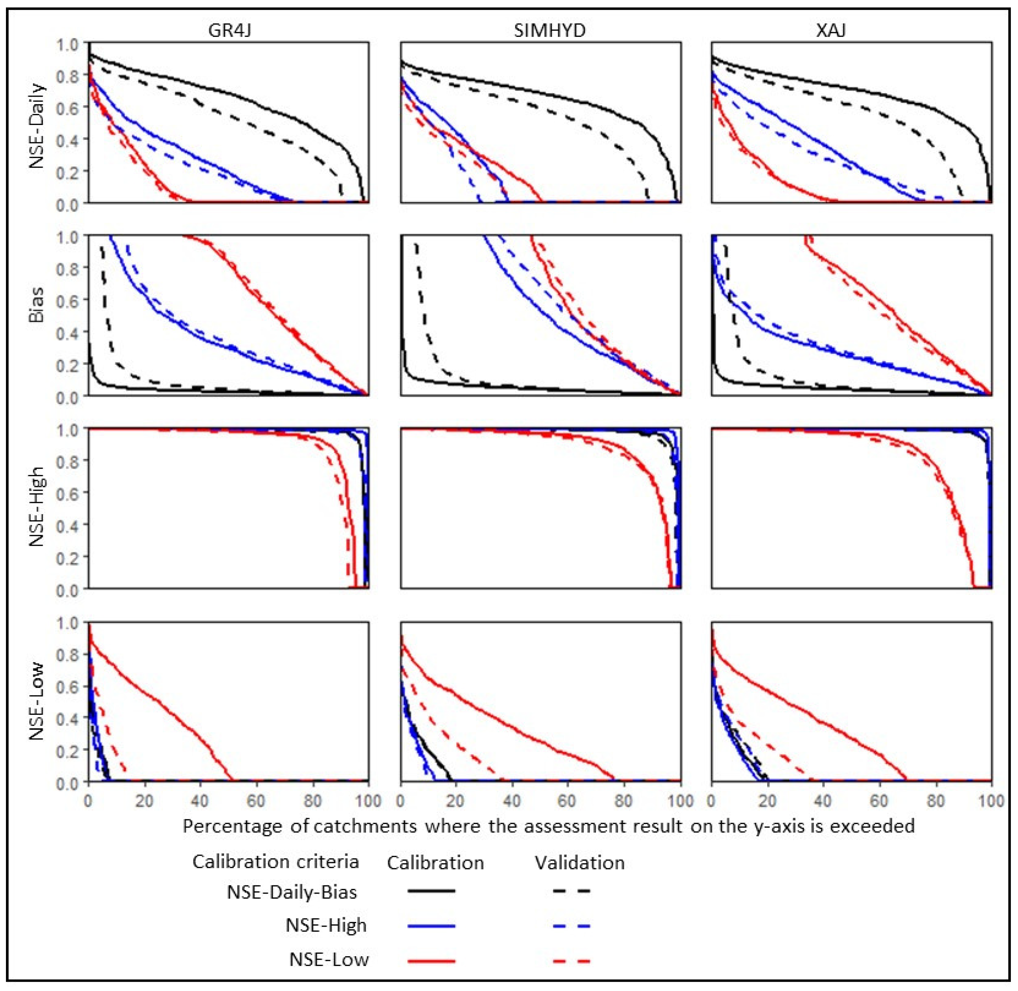
Figure 2 shows the model calibration and validation results for the three rainfall-runoff models. The results for the three rainfall-runoff models are very similar. As expected, the best results for each of the streamflow characteristics come from simulations using parameter values obtained from the calibration that specifically targets the streamflow characteristic that is being assessed. Also as expected, the calibration results are better than the validation results, by about 10–20% in the objective assessment criteria.
As with most hydrological modelling studies (see references in the Introduction and in Section 3.2), the results here show that the model calibration against NSE-Daily-Bias can simulate the daily streamflow and mean annual streamflow reasonably satisfactorily in most catchments (black lines in first two rows of Figure 2). The NSE-Daily in the model validation is greater than 0.5 in 60% of the 780 catchments. The Bias is less than 10% in 80% of the catchments (note that all the presentations and discussions in the paper refer to the absolute value of Bias). Both the model calibrations against NSE-High and NSE-Low show much poorer simulation (blue and red lines in first two rows of Figure 2).
The high flow simulations using parameter values from model calibration against NSE-Daily-Bias and against NSE-High are both very good (third row in Figure 2). The results from both calibrations are similar, with NSE-High being close to one in practically all the catchments (i.e., the model can reproduce the number of days in each year with streamflow above the 95th percentile daily streamflow). The high flow simulation with parameter values from model calibration against NSE-Low is also relatively good (NSE-High above 0.8 in most catchments), but poorer than the results from calibration against NSE-Daily-Bias and NSE-High.
The low flow simulations, defined here as the ability of the model to simulate the number of days in each year with streamflow below the 5th percentile daily streamflow, using parameter values from calibration against all three criteria are very poor. The best result comes from the calibration against NSE-Low, but even here, the NSE-Low is greater than zero in only 70% of the catchments for the SIMHYD and Xinanjiang models (and 50% for the GR4J model) in the model calibration, and 40% for the SIMHYD and Xinanjiang models (and 20% for the GR4J model) in the model validation.
3.2. Prediction in Ungauged Catchments
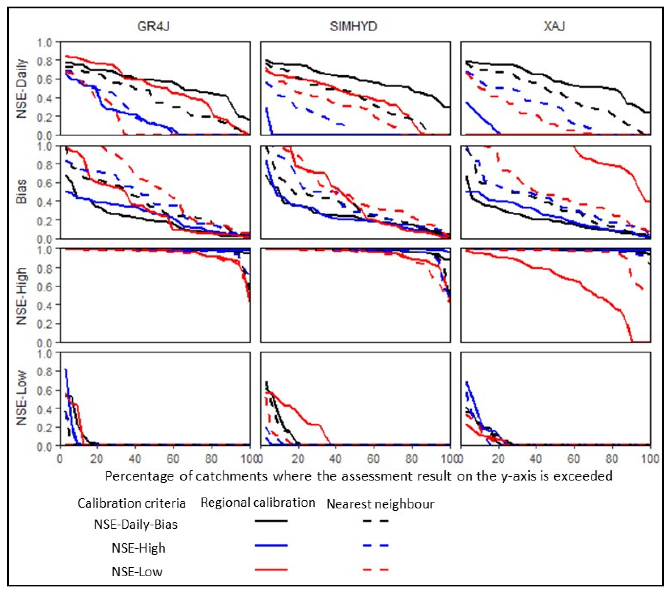
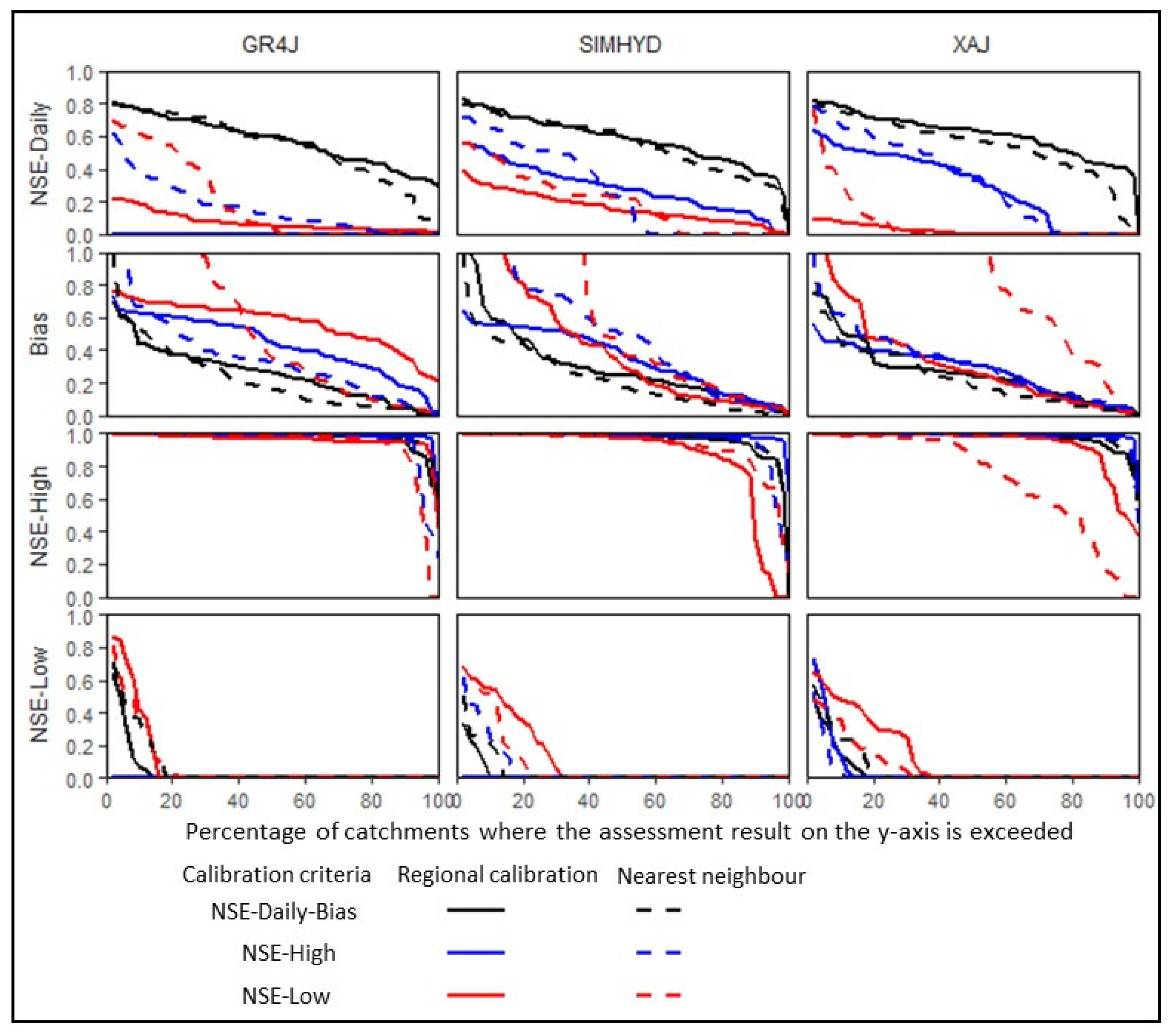
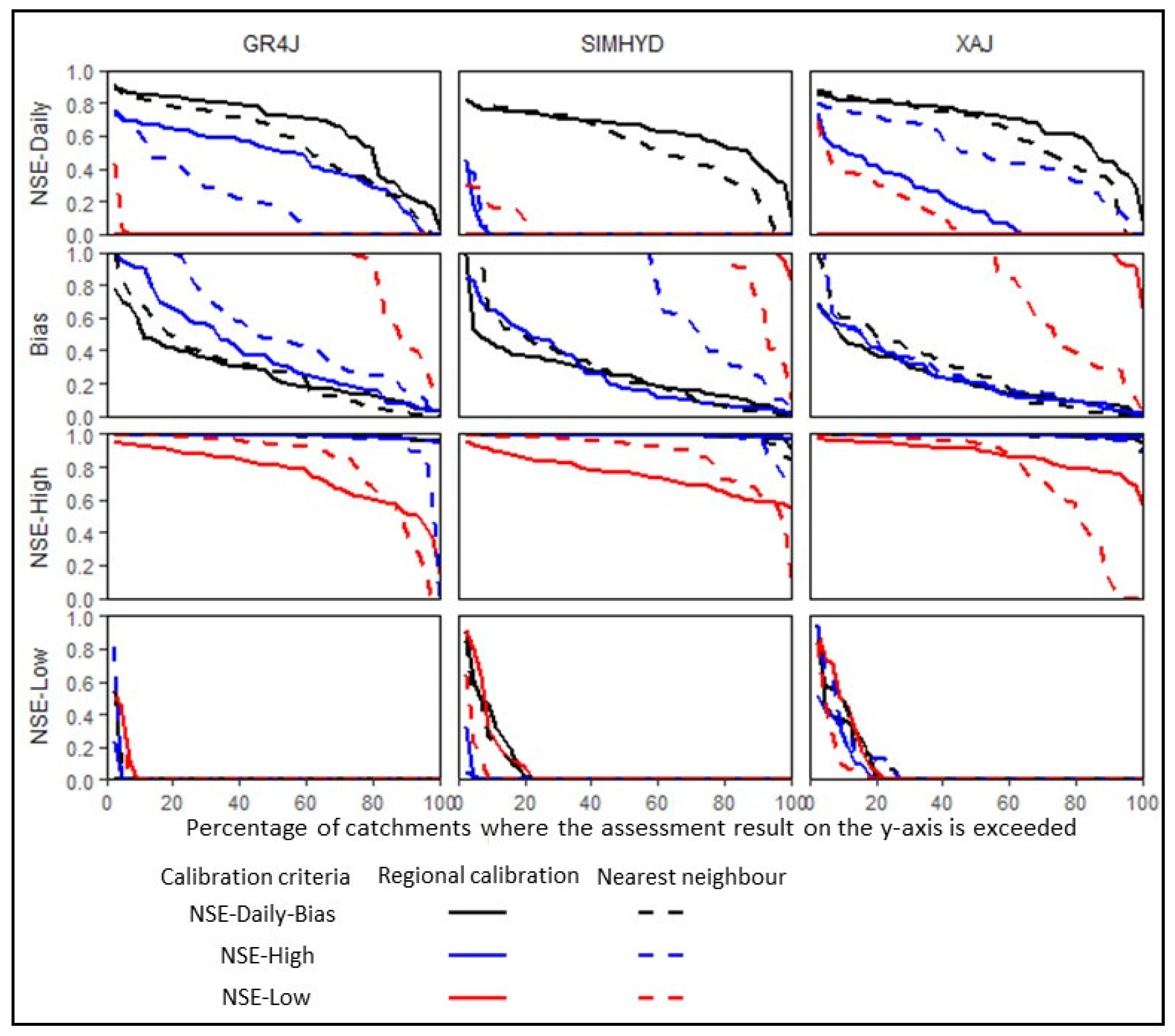
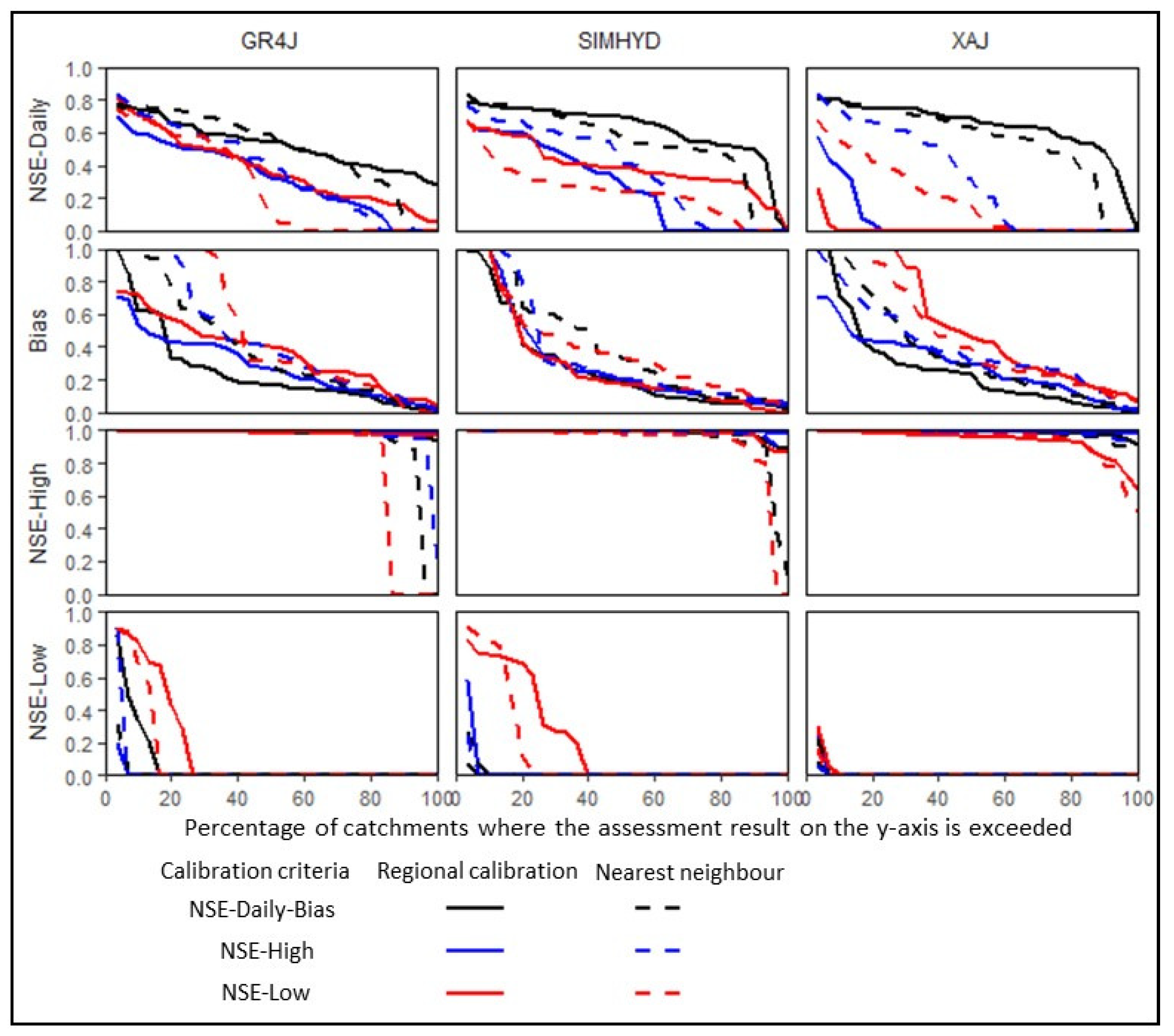
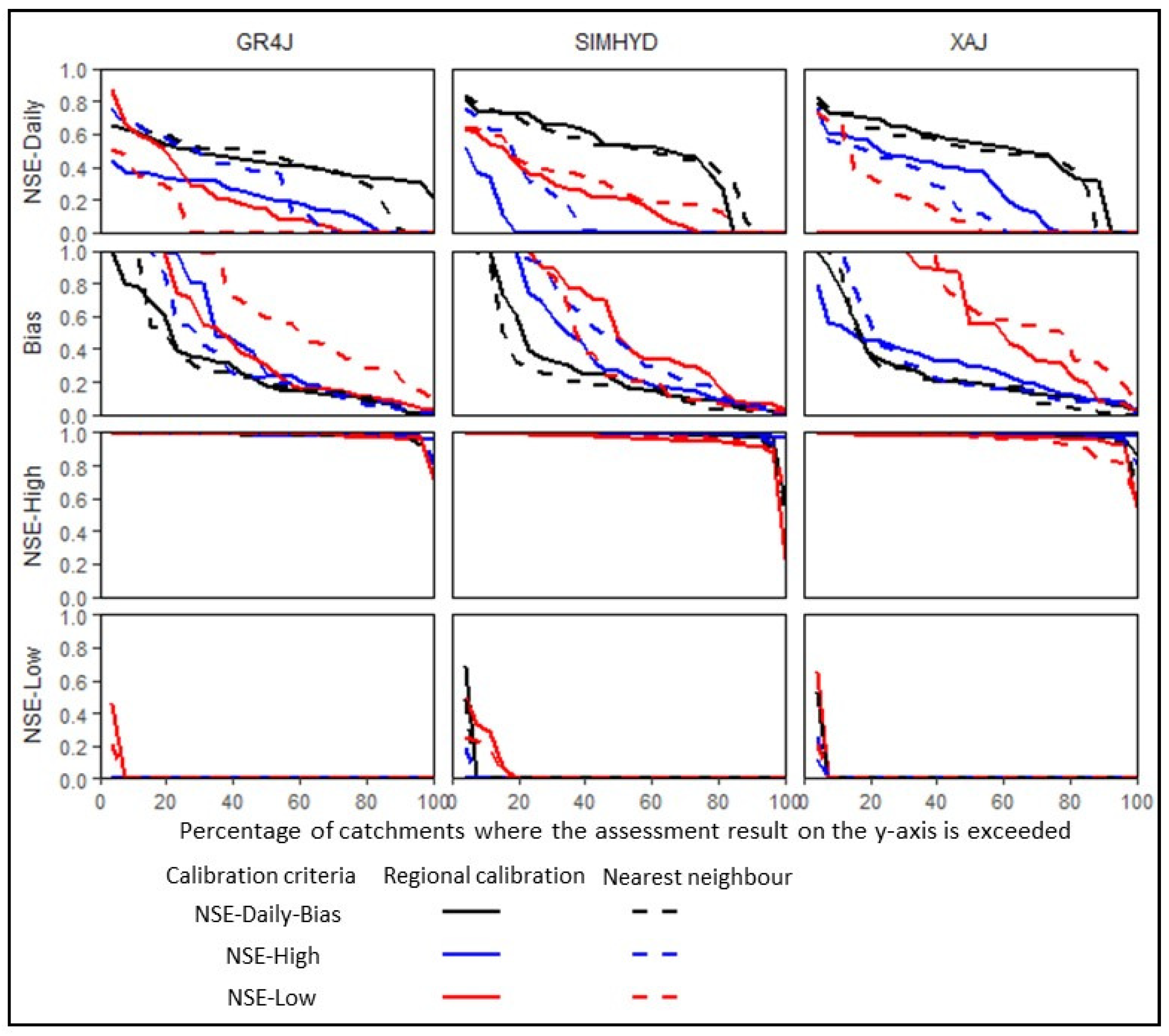
Figure 3, Figure 4, Figure 5, Figure 6 and Figure 7 show the results for streamflow prediction in ungauged catchments from the three rainfall-runoff models for the five regions. The plots show results from prediction using the “regional calibration” method (one single set of parameter values for the entire region) and “nearest neighbour” method (prediction using parameter values from the closest calibrated gauged catchment). To allow a direct comparison, the nearest neighbour results are also summarised for the same catchments used in the regional calibration (Figure 1). The general results from the three rainfall-runoff models are similar; however unlike the calibration and validation for single catchments in Section 2.1, the differences between models in predicting streamflow in ungauged catchments here are larger and significant.
As expected, the “prediction in ungauged catchment” results here are considerably poorer than the direct calibration for individual catchments in Section 3.1 (full lines in Figure 2). Nevertheless, the three models, using parameter values calibrated against NSE-Daily-Bias, can generally predict the daily streamflow and mean annual streamflow reasonably satisfactorily in many catchments. The NSE-Daily for daily streamflow prediction from the regional calibration for all regions (full black lines in the first row of Figure 3, Figure 4, Figure 5 and Figure 6) except northern Australia, is generally greater than 0.5 in more than 60% of the catchments. The runoff simulations for northern Australia (Figure 7) are slightly poorer, most likely because of the larger catchment areas in this region as the lumped modelling in this study does not rout the runoff. The Bias or error in the predicted mean annual streamflow is generally less than 20% in 50% of the catchments and less than 40% in 80% of the catchments (full black lines in the second row of Figure 3, Figure 4, Figure 5, Figure 6 and Figure 7). These results are consistent with similar studies with large data sets [7,8,9,21,27,28].
The daily streamflow and mean annual streamflow from the regional calibration is similar to or better than the simulation using parameter values from the nearest neighbour. The NSE-Daily from the regional calibration is generally higher than the NSE-Daily from nearest neighbour in far south-east Australia and south-west Australia (full black lines versus dashed black lines in the first row of Figure 3 and Figure 5). The Bias or error in the modelled mean annual streamflow is lower in the regional calibration than the nearest neighbour in far south-east Australia, far south-west Australia and north-east Australia (full black lines versus dashed black lines in the second row of Figure 3, Figure 5 and Figure 6).
Both the calibration against NSE-High and NSE-Low (blue and red lines in the first two rows of Figure 3, Figure 4, Figure 5, Figure 6 and Figure 7) generally perform poorly, and much poorer than the calibration against NSE-Daily-Bias, in predicting the daily streamflow series and mean annual streamflow in the ungauged catchments. There are several interesting observations with the modelling using parameter values from calibration against NSE-High and NSE-Low. The errors in mean annual streamflow are lower (lower Bias) in the simulations with NSE-High parameter values compared to simulations with NSE-Low parameter values because the average or total streamflow volume is influenced more by the high flow than the low flow. In fact, the modelled mean annual streamflow results from the regional calibration against NSE-High are comparable to those from the regional calibration against NSE-Daily-Bias in far south-east Australia, south-west Australia and north-east Australia (full blue lines versus full black lines in the second row of Figure 3, Figure 5 and Figure 6). However, the relative performance in simulating the daily streamflow time series (NSE-Daily result) using parameter values from calibration against NSE-High and NSE-Low can be very different in the different models and regions. This is likely because it is relatively easy to reproduce the high flow characteristic defined here (see NSE-High results below), and many different sets of parameter values can give similarly good simulations when the model is calibrated against NSE-High. By contrast, it is difficult to simulate the low flow characteristic defined here (see NSE-Low results below) leading to a more unique set of parameter values when the model is calibrated against NSE-Low, resulting in the NSE-Low calibration showing better prediction of daily streamflow (NSE-Daily-Bias) than the NSE-High calibration in some regions.
As in the model calibration and validation on individual catchments in Section 3.1, all the modelling methods can reproduce the high flow characteristic, defined here as the ability to simulate the number of days in each year with streamflow above the 95th percentile daily streamflow (measured by NSE-High). The predictions using parameter values from the regional calibration and nearest neighbour methods for calibration against NSE-Daily-Bias and NSE-High led to NSE-High values close to one in practically all the catchments (third row in Figure 3, Figure 4, Figure 5, Figure 6 and Figure 7). The prediction of high flow in ungauged catchments from model calibration against NSE-Low are also generally good, except perhaps for far south-west Australia. The prediction of low flow in ungauged catchments, defined here as the ability to simulate the number of days in each year with streamflow below the 5th percentile daily streamflow (measured by NSE-Low), from all three models and calibration methods are very poor (bottom row in Figure 3, Figure 4, Figure 5, Figure 6 and Figure 7).
3.3. Modelling Climate Change Impact on Streamflow Characteristics
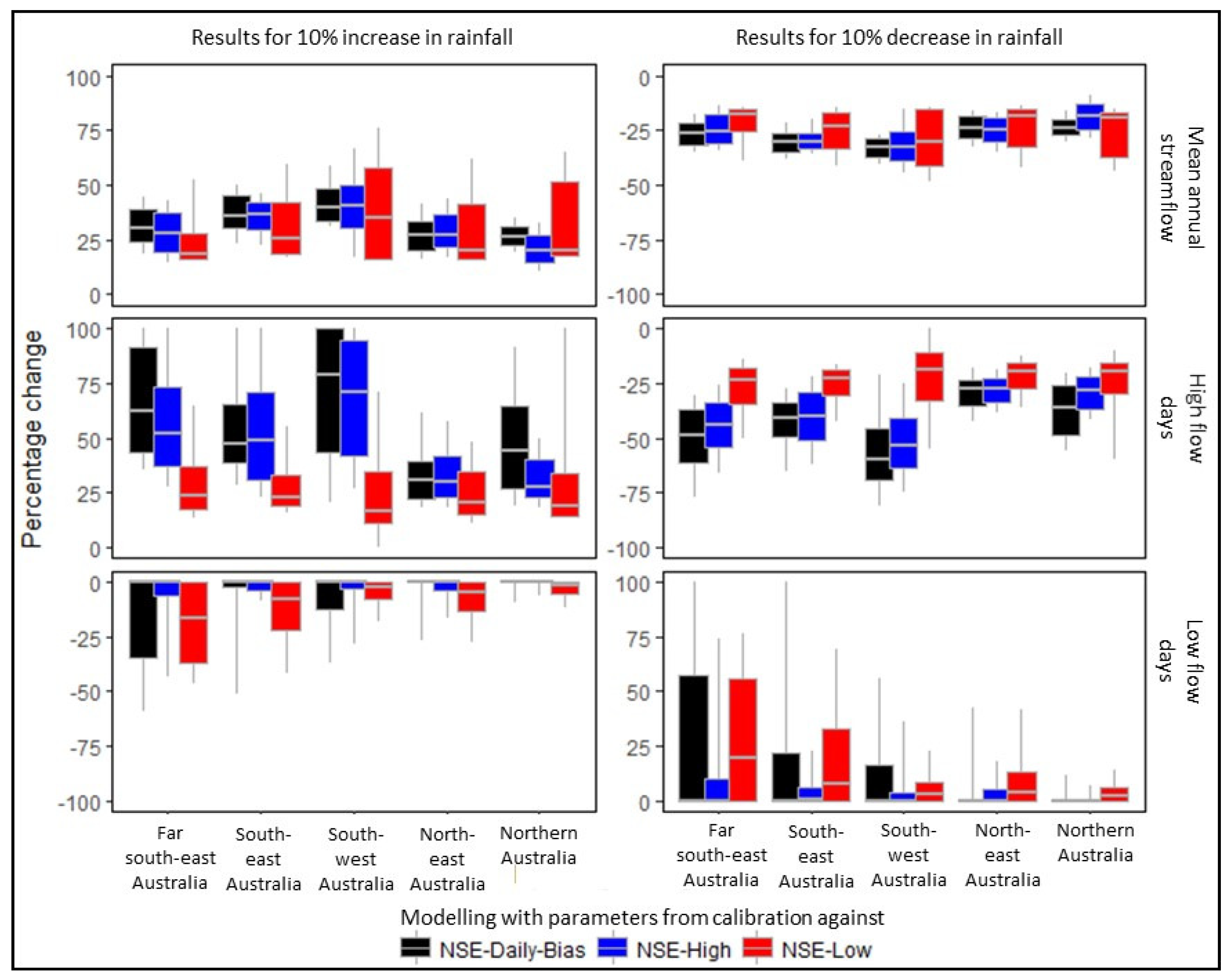
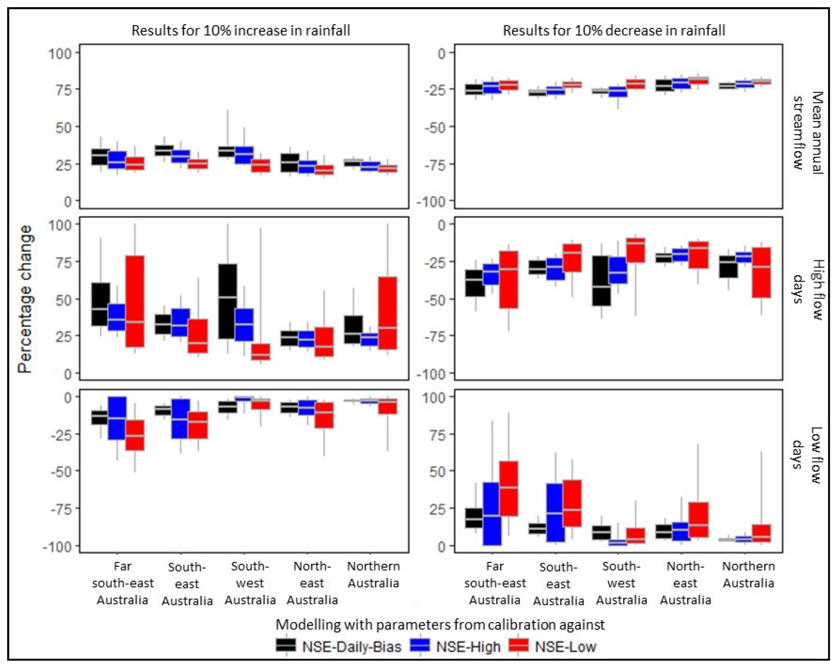
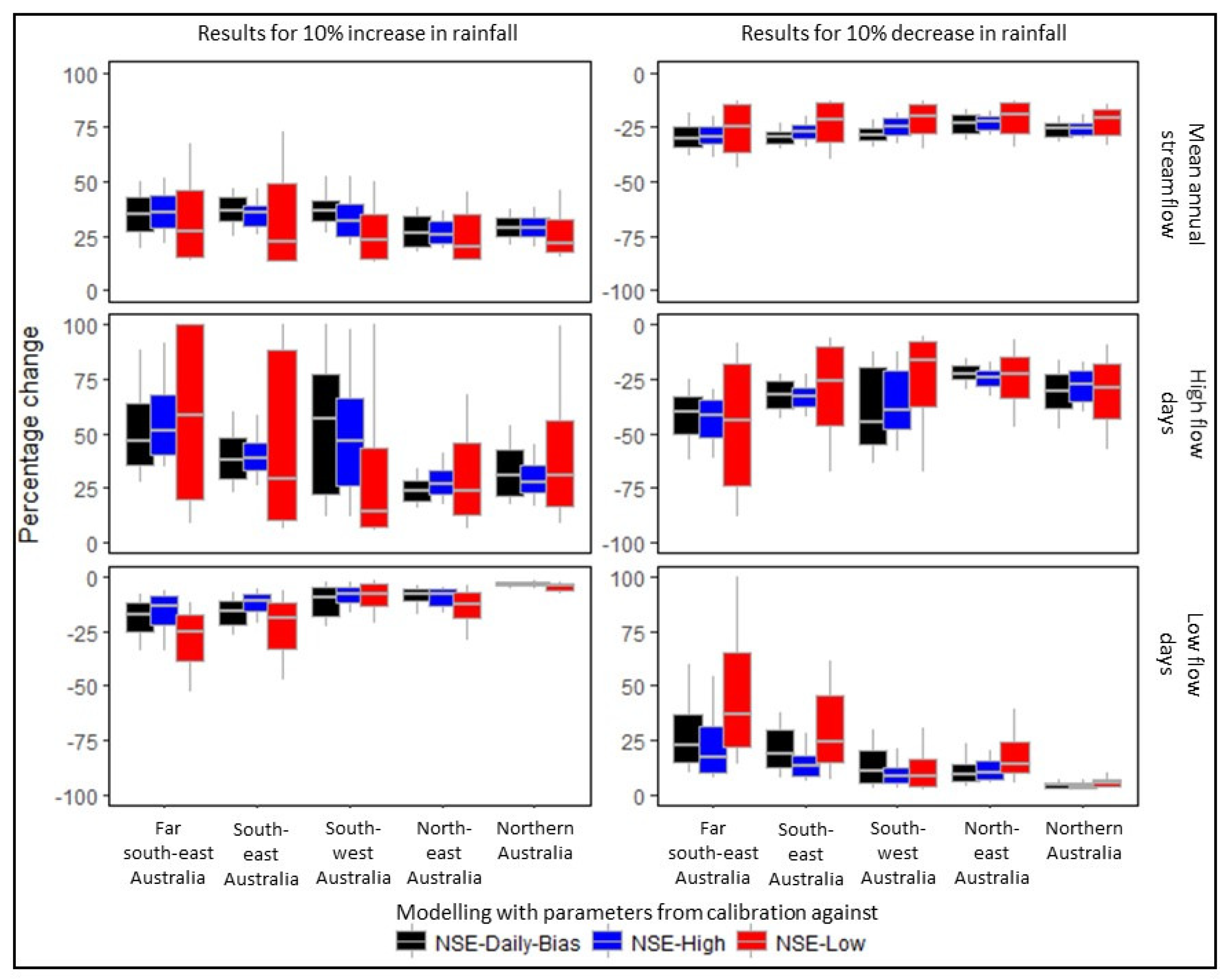
Figure 8, Figure 9 and Figure 10 show the rainfall sensitivity modelling results from the GR4J, SIMHYD and Xinanjiang models, respectively. The plots show the range of results from the catchments in the five regions from modelling with parameter values from model calibrations against NSE-Daily-Bias, NSE-High and NSE-Low. The number of catchments in each region varies from 82 to 286 (Figure 1) and is more than the subset of catchments used for the regional calibration modelling experiment in Section 3.2. The plots present the impact of a + 10% and a − 10% change in rainfall (the same scaling is applied to all the 1981–2010 daily rainfalls, see Section 2.3) on the mean annual streamflow, number of high flow days (number of days with streamflow above the 95th percentile daily streamflow), and number of low flow days (number of days with streamflow below the 5th percentile daily streamflow). The 5th and 95th percentile daily streamflow thresholds are calculated from the historical 1981–2010 data. The results, as expected, show that a rainfall increase will lead to higher mean annual streamflow, more high flow days, and fewer low flow days, and the opposite for a rainfall decrease.
For modelled change in mean annual streamflow using NSE-Daily-Bias parameter values (i.e., parameter values from model calibration against NSE-Daily-Bias) (black bars in the top row of Figure 8, Figure 9 and Figure 10), the SIMHYD model shows the least variation between the different regions and between catchments within a region. The biggest variation or range in the results come from the GR4J model. In general, the 10% change in rainfall is amplified as a 20–30% change in mean annual streamflow, and up to 40% in the GR4J and Xinanjiang models. The modelled rainfall elasticity of streamflow (percent change in streamflow relative to the percent change in rainfall, [29]) is generally higher for a rainfall increase than a rainfall decrease, particularly in the GR4J and Xinanjiang models. The rainfall elasticity of streamflow is lowest in the wet tropics (north-east Australia and northern Australia) and highest in south-west Australia.
The rainfall elasticity of streamflow from modelling with NSE-High parameter values is lower than from modelling with NSE-Daily-Bias parameter values in most regions in the Xinanjiang model and for rainfall increases in the SIMHYD model (black and blue bars in the top row of Figure 8, Figure 9 and Figure 10). The modelling with NSE-High parameter values compared to modelling with NSE-Daily-Bias parameter values shows a bigger range in the results in the GR4J model, but similar range of results in the SIMHYD and Xinanjiang models. The rainfall elasticity of streamflow from modelling with NSE-Low parameter values (red bars in the top row of Figure 8, Figure 9 and Figure 10) is considerably lower, and shows a much bigger range in results, than from modelling with both the NSE-Daily-Bias and NSE-High parameter values, in all three models and in all regions. However, the prediction from NSE-Low parameter values for mean annual streamflow and high flow days are likely to be poor (and much poorer than the predictions from NSE-Daily-Bias and NSE-High parameter values) given the poor NSE-Low calibration results (see Section 3.2), and the projections are shown here simply to illustrate differences that can arise from modelling with parameter values from different calibration criteria.
For modelled change in high flows, the modelling with NSE-Daily-Bias parameter values and NSE-High parameter values show relatively comparable results (black and blue bars in the middle row of Figure 8, Figure 9 and Figure 10). The range in the modelled change in high flow days across catchments within each region is generally smaller for predictions with NSE-High parameter values compared to predictions using NSE-Daily-Bias parameter values. This suggests that modelling with parameter values from model calibration against an objective function like NSE-High that specifically targets the high flow characteristic is likely to provide more robust prediction of climate change impact on high flow characteristic.
The median results from the SIMHYD model (blue bars in Figure 9) show that the 10% increase in rainfall led to about 25% increase in high flow days (number of days with streamflow above the 95th percentile daily streamflow) in northern Australia and about 35% increase in southern Australia. The median results from the Xinanjiang model (blue bars in Figure 10) from a 10% increase in rainfall show about 30% increase in high flow days in northern Australia and 40–50% increase in southern Australia. The modelled change in high flow days is higher in the GR4J model (blue bars in Figure 8) (30% median increase in northern Australia and 50–70% increase in southern Australia) compared to the SIMHYD and Xinanjiang models. The variation or range of modelled change in high flow days between catchments and regions is also higher in the GR4J model compared to the other two models.
The modelled change in high flow days using NSE-Low parameter values (red bars in the middle row of Figure 8, Figure 9 and Figure 10) are very different, and show a much bigger range of results between catchments and regions, compared to the modelling with NSE-Daily-Bias and NSE-High parameter values. For the GR4J model (and broadly also for the other two models), the modelled increase in high flow days from a 10% rainfall increase, and the modelled decrease in high flow days from a 10% rainfall decrease, is much lower from the NSE-Low parameter values compared to the NSE-Daily-Bias and NSE-High parameter values (middle row of Figure 8). Again, as mentioned above, there is little confidence in the predictions from NSE-Low parameter values because of the very poor model calibration against the NSE-Low objective criteria.
For modelled change in low flow days (number of days with streamflow below the 5th percentile daily streamflow), the different models and the model calibrations against different objective criteria give very different results (bottom row of Figure 8, Figure 9 and Figure 10). The biggest change in the number of low flow days almost always come from modelling with NSE-Low parameter values (red bars in bottom row of Figure 8, Figure 9 and Figure 10). The modelling with NSE-Low parameter values shows that the 10% increase in rainfall led to median results of 25% decrease in low flow days in the far-south east, 15% decrease in the south-east and 5–10% decrease elsewhere, and the 10% decrease in rainfall led to median results of 40% increase in low flow days in the far south-east, 30% increase in the south-east and 10–20% increase elsewhere. The modelled change in low flow days is generally smaller in the GR4J model compared to the SIMHYD and Xinanjiang models, where a large number of catchments, particularly in the north-east and northern Australia, show little change in low flow days from the 10% rainfall change.
4. Discussion
4.1. Hydrological Prediction in Ungauged Catchments
The results show that parameter values from model calibration against NSE-Daily-Bias can generally adequately simulate daily streamflow series and mean annual streamflow, for an independent test period and for ungauged catchments. The results are consistent with similar studies with large data sets (see references in the Introduction and in Section 3.2), where calibrating a model against an objective criteria like the NSE-Daily-Bias which reflects the simulation of medium and high daily streamflow, will produce parameter values that can generally adequately simulate the daily streamflow time series and mean annual streamflow. It is also interesting to note that the daily streamflow simulations with parameter values from regional calibration is generally better than the simulations with parameter values from the closest gauged catchment calibration. The relatively good performance of the regional calibration is likely due to the regions being relatively hydrologically similar, and because the parameterisation using datasets from across a region may overcome error or uncertainty that can arise from using parameter values from an adjacent catchment that is very different or poorly calibrated.
The NSE-Daily-Bias parameter values also predict very well the high flow characteristic, defined here as the number of days in each year with streamflow above the 95th percentile daily streamflow. In fact, parameter values from model calibrations against NSE-Daily-Bias and against NSE-High, which directly reflects the high flow characteristic that is assessed here, produce almost perfect simulation of the high flow days, with the NSE-High value being close to one in practically all the catchments. The parameter values from calibration against NSE-Low, which has little resemblance to high flow prediction, also managed to predict the high flow days reasonably well. These suggest that the medium and high flow characteristics or signatures are relatively easier to predict. As such, for simulations of streamflow series and medium and high flow characteristics (for example, long-term average volume, daily flows above the 50th percentile, multi-day medium and high flow events, etc.), a single set of unique parameter values from model calibration against an objective function like the NSE-Daily-Bias can be used for consistency in the simulation and interpretation of the different streamflow characteristics. However, it should be noted that this may not necessarily apply to very high extreme flows or events with low return periods (e.g., 1 in 1 year and less frequent events) [13,14].
The prediction of low flow is altogether a different story. None of the model calibrations can reproduce the low flow characteristic explored here (number of days in each year with streamflow below the 5th percentile daily streamflow), including calibrating against an objective function that specifically targets this characteristic. It is likely that the low flow characteristic defined here is difficult to simulate, and there has been some success in predicting other low flow characteristics (for example, low flow percentiles, zero flows days, etc.), particularly when regression models that relate the low flow characteristic to catchment attributes are used to directly predict the low flow characteristic [12,30]. Nevertheless, the results here indicate that low flow characteristics are considerably more difficult to predict, and reliable prediction requires careful modelling consideration that specifically targets the low flow characteristic of interest. The definition of the low flow characteristic to reflect the objective of a specific study must also be more precise than the example used here, including accounting for long periods of zero flow days in ephemeral rivers (e.g., south-west Australia) and seasonality (e.g., many rivers in northern Australia have little flow in winter, and many rivers in south-west Australia have little flow in summer).
4.2. Hydrological Prediction under Climate Change
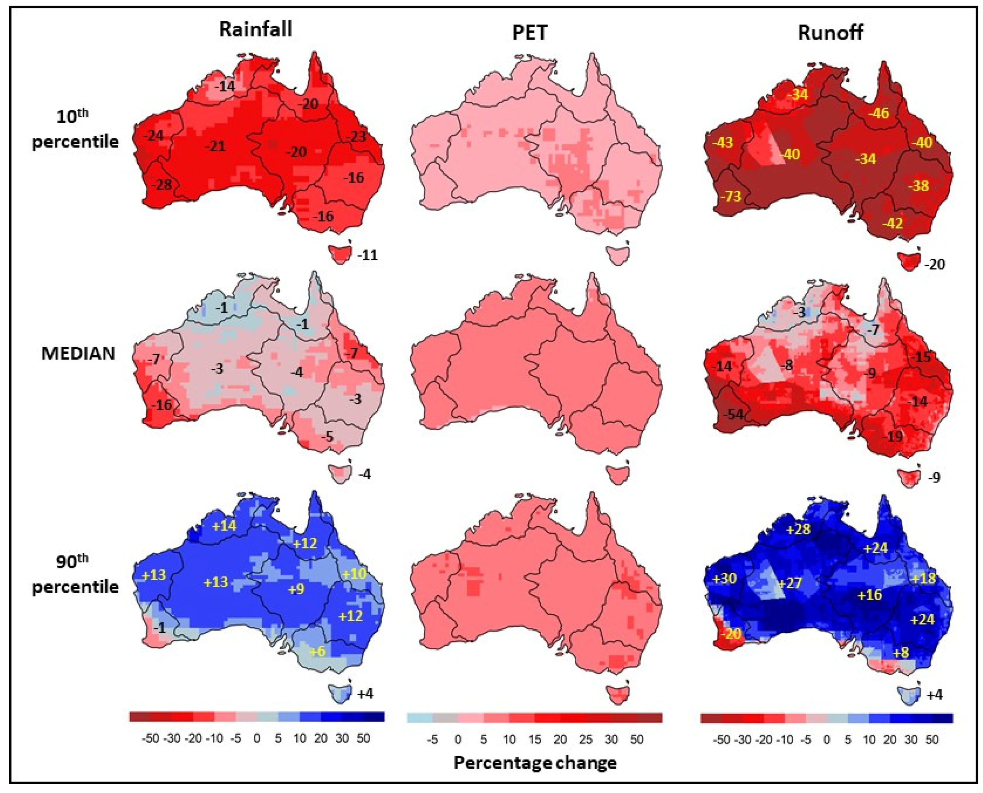
The sensitivity modelling experiment in this study, where the entire 1981–2010 daily rainfall series is perturbed or scaled by +10% and -10%, is carried out to explore the implications of model choice and calibration method on the prediction of climate change impact on streamflow characteristics. Before discussing the results from this simplistic modelling experiment, Figure 11 provides some context around the most recent climate and runoff projections for Australia. The plots show projected changes in rainfall, potential evapotranspiration (PET) and modelled runoff for 2046–2075 relative to 1976–2005 for RCP8.5 (highest Representative greenhouse gas Concentration Pathway). The range of projections (shown as 10th percentile, median, and 90th percentile values) are informed by the 42 CMIP5 (Coupled Model Intercomparison Project Phase 5) global climate models used in the Intergovernmental Panel on Climate Change Fifth Assessment Report (IPCC AR5). These projections for Australia come from [31], which also discuss in some detail the challenges and opportunities in modelling climate change impacts on hydrological fluxes and stores.
There is general agreement in the PET projections with about 2.5 °C warming in 2046–2075 for RCP8.5 leading to about 10–15% increase in PET. However, there is considerable uncertainty in the rainfall projections, where the 10th and 90th percentile projections generally differ by up to 50%, and this is amplified in the modelled runoff. Nevertheless, there is strong agreement in the projections for declining runoff in the far south-west (median projection of 50% decline in mean annual runoff, with extreme dry projection of 70% reduction) and far south-east (median projection of 20% decline in mean annual runoff, with extreme dry projection of 40% reduction) where the large majority of global climate models project a drier future winter when most of the runoff in these regions occurs [25,31,32]. However, the direction of rainfall and runoff change is less certain in other parts of Australia (−40% to +30% change in mean annual runoff in northern Australia, and −40% to +20% in eastern Australia).
Returning to the sensitivity modelling experiment in this study, the results show that the predicted change in the various streamflow characteristics from the different models and using parameter values from the different calibration criteria can be quite different. The strongest agreement between models is in the predicted change in mean annual streamflow using parameter values from calibration against NSE-Daily-Bias. The disagreement between models in the predicted change in mean annual streamflow is also likely to be smaller than the range of rainfall projections from the different climate models ([33] and Figure 11).
Results from the different models and the different calibration criteria differ significantly for the predicted change in high flow days, and even more so for the low flow days. Unlike the long-term averages, the differences in future projections of these streamflow characteristics from different rainfall-runoff models and calibration methods can be larger than the range or uncertainty in the future rainfall projections. There is also much less confidence in the projections of climate change impact on low flows presented here given the very poor model calibrations against the low flow characteristic considered here.
The differences in the projections of the high and low flow characteristics are largely due to the different process conceptualisations in the different models, particularly the simulation of evapotranspiration, which will manifest more in the prediction of the tails of the streamflow distribution compared to the long-term mean streamflow. For example, the results from the GR4J model are considerably different to the results from the SIMHYD and Xinanjiang models, likely because the SIMHYD and Xinanjiang models force a closed catchment water balance while the GR4J model allows for the simulation of water leaving or coming into the catchment.
The results here have significant implications on modelling the impact of climate change on the different streamflow characteristics. It is likely that the difference between the predicted streamflow change reported here will be even greater if changes to the different parts of the daily rainfall distribution and other rainfall characteristics (rather than a constant scaled change applied to all the daily rainfall amounts here), as well as changes to temperature and/or potential evapotranspiration, are considered. The differences between models will also be enhanced when the models are adapted and new process conceptualisations introduced to enable extrapolation of the model to predict a future under higher temperature, higher CO2, and changed hydrologic regime [25]. In any case, from a rainfall-runoff modelling perspective, climate impact modelling should at the very least use parameter values from model calibration against an objective criteria that specifically targets the streamflow characteristic that is being assessed.
5. Summary and Conclusions
The paper investigates the prediction of different streamflow characteristics in ungauged catchments and under changes in the rainfall inputs, with three lumped conceptual daily rainfall-runoff models calibrated against three different objective criteria, using a large data set from 780 catchments across Australia. The results indicate that medium and high flows are relatively easier to predict, suggesting that using a single unique set of parameter values from model calibration against an objective criteria like the Nash–Sutcliffe efficiency is adequate and desirable to provide a consistent simulation and interpretation of daily streamflow series and the different medium and high flow characteristics. However, the low flow characteristics are considerably more difficult to simulate, and will require careful modelling consideration, in both the model conceptualisation and calibration as well as the precise definition of the low flow characteristic, to specifically target the low flow characteristic of interest. These observations are consistent for all the three rainfall-runoff models used here.
The sensitivity modelling experiment indicates that different rainfall-runoff models and different calibration and parameterisation approaches can give different predictions of climate change impact on streamflow characteristics. The models agree most in the prediction or projection of long-term average characteristics like the mean annual streamflow, where the difference between rainfall-runoff model simulations is likely to be smaller than the uncertainty in the future rainfall projections. However, the modelled changes in streamflow characteristics beyond the long-term averages, particularly the low flow characteristics, can differ significantly between rainfall-runoff models and different calibration approaches. As such, climate change impact modelling will require careful modelling consideration and calibration against appropriate objective criteria that specifically targets the streamflow characteristic that is being assessed.
Author Contributions
F.H.S.C, H.Z. and N.J.P. designed and interpreted the modelling experiments. H.Z. performed the modelling experiments. H.Z. and F.H.S.C. analysed the data. F.H.S.C. wrote the paper.
Acknowledgments
This study is supported by the Australian Commonwealth Scientific and Industrial Research Organisation, the Victorian Department of Land and Water Planning, and the Earth Systems and Climate Change Hub. Results from this and related studies are being used to develop improved projections of water futures to support planning and adaptation in the water and related sectors. The authors like to thank the journal academic editor and external reviewers for their feedback, which improved this paper.
Conflicts of Interest
The authors declare no conflict of interest.
References
- Beven, K.J. Rainfall-Runoff Modelling—The Primer; Wiley: West Sussex, UK, 2001; 360p. [Google Scholar]
- Bloschl, G.; Sivapalan, M.; Wagener, T.; Viglione, A.; Savenije, H. Runoff Prediction in Ungauged Basins—Synthesis across Processes, Places and Scales; Cambridge University Press: Cambridge, UK, 2013; 465p. [Google Scholar]
- Chiew, F.H.S.; Teng, J.; Vaze, J.; Post, D.A.; Perraud, J.-M.; Kirono, D.G.C.; Viney, N.R. Estimating climate change impact on runoff across south-east Australia: Method, results and implications of modelling method. Water Resour. Res. 2009, 45, W10414. [Google Scholar] [CrossRef]
- Chiew, F.H.S. Lumped conceptual rainfall-runoff models and simple water balance methods: Overview and applications in ungauged and data limited regions. Geogr. Compass 2010, 4, 206–225. [Google Scholar] [CrossRef]
- Parajka, J.; Bloschl, G. The value of MODIS snow cover data in validating and calibrating conceptual hydrological models. J. Hydrol. 2008, 358, 240–258. [Google Scholar] [CrossRef]
- Zhang, Y.Q.; Chiew, F.H.S.; Zhang, L.; Li, H.X. Use of remotely sensed actual evapotranspiration to improve rainfall-runoff modelling in southeast Australia. J. Hydrometeorol. 2009, 10, 969–980. [Google Scholar] [CrossRef]
- Oudin, L.; Andreassian, V.; Perrin, C.; Michel, C.; Le Moine, N. Spatial proximity, physical similarity, regression and ungauged catchments: A comparison of regionalisation approaches based on 913 French catchments. Water Resour. Res. 2008, 44, W03413. [Google Scholar] [CrossRef]
- Zhang, Y.Q.; Chiew, F.H.S. Relative merits of different methods for runoff predictions in ungauged catchments. Water Resour. Res. 2009, 45, W07412. [Google Scholar] [CrossRef]
- Parajka, J.; Bloschl, G.; Merz, R. Regional calibration of catchment models: Potential for ungauged catchments. Water Resour. Res. 2007, 43, W06406. [Google Scholar] [CrossRef]
- Nash, J.E.; Sutcliffe, J.V. River flow forecasting through conceptual models part I—A discussion of principles. J. Hydrol. 1970, 10, 282–290. [Google Scholar] [CrossRef]
- Gupta, H.V.; Kling, H.; Yilmaz, K.K.; Martinez, G.F. Decomposition of the mean squared error and NSE performance criteria: Implications for improving hydrological modelling. J. Hydrol. 2009, 377, 80–91. [Google Scholar] [CrossRef] [Green Version]
- Laaha, G.; Demuth, S.; Hisdal, H.; Kroll, C.N.; van Lanen, H.A.J.; Nester, T.; Rogger, M.; Sanquet, E.; Tallaksen, L.M.; Woods, R.A.; et al. Prediction of low flows in ungauged basins. In Runoff Prediction in Ungauged Basins; Bloschl, G., Sivapalan, M., Wagener, T., Viglione, A., Savinije, H., Eds.; Cambridge University Press: Cambridge, UK, 2009; pp. 163–188. [Google Scholar]
- Rosbjerg, D.; Bloschl, G.; Burn, D.H.; Castellarin, A.; Croke, B.; Di Baldassarre, G.; Iacobellis, V.; Kjeldsen, T.R.; Kuczera, G.; Merz, R.; et al. Prediction of floods in ungauged basins. In Runoff Prediction in Ungauged Basins; Bloschl, G., Sivapalan, M., Wagener, T., Viglione, A., Savinije, H., Eds.; Cambridge University Press: Cambridge, UK, 2009; pp. 189–226. [Google Scholar]
- Tan, K.S.; Chiew, F.H.S.; Grayson, R.B.; Scanlon, P.J.; Siriwardena, L. Calibration of a daily rainfall-runoff model to estimate high daily flows. In Proceedings of the MODSIM 2005 International Congress on Modelling and Simulation, Melbourne, Australia, 12–15 December 2005; pp. 2960–2966. [Google Scholar]
- Perrin, C.; Michel, C.; Andreassian, V. Improvement of a parsimonious model for streamflow simulation. J. Hydrol. 2003, 279, 275–289. [Google Scholar] [CrossRef]
- Chiew, F.H.S.; Peel, M.C.; Western, A.W. Application and testing of the simple rainfall-runoff model SIMHYD. In Mathematical Models of Small Watershed Hydrology and Applications; Singh, V.P., Frevert, D.K., Eds.; Water Resources Publication: Littleton, CO, USA, 2002; pp. 335–367. [Google Scholar]
- Zhao, R.J. The Xinanjiang model applied in China. J. Hydrol. 1992, 135, 371–381. [Google Scholar]
- Jeffrey, S.J.; Carter, J.O.; Moodie, K.B.; Beswick, A.R. Using spatial interpolation to construct a comprehensive archive of Australian climate data. Environ. Model. Softw. 2001, 16, 309–330. [Google Scholar] [CrossRef]
- Morton, F.I. Operational estimates of areal evapotranspiration and their significance to the science and practice of hydrology. J. Hydrol. 1983, 66, 1–76. [Google Scholar] [CrossRef]
- Chiew, F.H.S.; McMahon, T.A. The applicability of Morton’s and Penman’s evapotranspiration estimates in rainfall-runoff modelling. Water Resour. Bull. 1991, 27, 611–620. [Google Scholar] [CrossRef]
- Vaze, J.; Chiew, F.H.S.; Perraud, J.-M.; Viney, N.; Post, D.; Teng, J.; Wang, B.; Lerat, J.; Goswomi, M. Rainfall-runoff modelling across southeast Australia: Datasets, models and results. Australas. J. Water Resour. 2011, 14, 101–116. [Google Scholar] [CrossRef]
- Viney, N.R.; Perraud, J.; Vaze, J.; Chiew, F.H.S.; Post, D.A.; Yang, A. The usefulness of bias constraints in model calibration for regionalisation to ungauged catchments. In Proceedings of the MODSIM2009 International Congress on Modelling and Simulation, Cairns, Australia, 13–17 July 2009; pp. 3421–3427. [Google Scholar]
- Poff, N.L.; Richter, B.D.; Arthington, A.H.; Bunn, S.E.; Naiman, R.J.; Kendy, E.; Acreman, M.; Apse, C.; Bledsoe, B.P.; Freeman, M.C. The ecological limits of hydrologic alteration (ELOHA): A new framework for developing regional environmental flow standards. Freshw. Biol. 2010, 55, 147–170. [Google Scholar] [CrossRef]
- Rolls, R.J.; Leigh, C.; Sheldon, F. Mechanistic effects of low-flow hydrology on riverine ecosystems: Ecological principles and consequences of alteration. Freshw. Sci. 2012, 31, 1163–1186. [Google Scholar] [CrossRef]
- Chiew, F.H.S.; Potter, N.J.; Vaze, J.; Petheram, C.; Zhang, L.; Teng, J.; Post, D.A. Observed hydrologic non-stationarity in far south-eastern Australia: Implications and future modelling predictions. Stoch. Environ. Res. Risk Assess. 2014, 28, 3–15. [Google Scholar] [CrossRef]
- Vaze, J.; Post, D.A.; Chiew, F.H.S.; Perraud, J.-M.; Viney, N.; Teng, J. Climate non-stationarity—Validity of calibrated rainfall-runoff models for use in climate change studies. J. Hydrol. 2010, 394, 447–457. [Google Scholar] [CrossRef]
- Merz, R.; Bloschl, G. Regionalisation of catchment model parameters. J. Hydrol. 2004, 287, 95–123. [Google Scholar] [CrossRef] [Green Version]
- Viney, N.; Vaze, J.; Crosbie, R.; Wang, B.; Dawes, W.; Frost, A. AWRA-L v5.0: Technical Description of Model Algorithms and Inputs; Commonwealth Scientific and Industrial Research Organisation: Canberra, Australia, 2015; 76p.
- Chiew, F.H.S. Estimation of rainfall elasticity of streamflow in Australia. Hydrol. Sci. J. 2006, 51, 613–625. [Google Scholar] [CrossRef] [Green Version]
- Zhang, Y.Q.; Vaze, J.; Chiew, F.H.S.; Teng, J.; Li, M. Predicting hydrological signatures in ungauged catchments using spatial interpolation, index model and rainfall-runoff modelling. J. Hydrol. 2014, 517, 936–948. [Google Scholar] [CrossRef]
- Chiew, F.H.S.; Zheng, H.; Potter, N.J.; Ekstrom, M.; Grose, R.; Kirono, D.G.C.; Zhang, L.; Vaze, J. Future runoff projections for Australia and science challenges in producing next generation projections. In Proceedings of the MODSIM2017 International Congress on Modelling and Simulation, Hobart, Australia, 3–8 December 2017; pp. 1745–1751. [Google Scholar]
- Potter, N.J.; Chiew, F.H.S. An investigation into changes in climate characteristics causing the recent very low runoff in the southern Murray-Darling Basin using rainfall-runoff models. Water Resour. Res. 2011, 47, W00G10. [Google Scholar] [CrossRef]
- Teng, J.; Vaze, J.; Chiew, F.H.S.; Wang, B.; Perraud, J.-M. Estimating the relative uncertainties sourced from GCMs and hydrological models in modelling climate change impact on runoff. J. Hydrometeorol. 2012, 13, 122–139. [Google Scholar] [CrossRef]
Figure 1.
Locations of 780 catchments used in this study.

Figure 2.
Calibration and validation results for the three rainfall-runoff models showing percentage of the 780 catchments with assessment results for the four streamflow characteristics exceeding the values on the y-axis.
Figure 2.
Calibration and validation results for the three rainfall-runoff models showing percentage of the 780 catchments with assessment results for the four streamflow characteristics exceeding the values on the y-axis.

Figure 3.
Prediction in ungauged catchment results for far south-east Australia for the three rainfall-runoff models from regional calibration parameters and nearest neighbour parameters, showing percentage of catchments with assessment results for the four streamflow characteristics exceeding the values on the y-axis.

Figure 4.
Prediction in ungauged catchment results for south-east Australia for the three rainfall-runoff models from regional calibration parameters and nearest neighbour parameters, showing percentage of catchments with assessment results for the four streamflow characteristics exceeding the values on the y-axis.

Figure 5.
Prediction in ungauged catchment results for far south-west Australia for the three rainfall-runoff models from regional calibration parameters and nearest neighbour parameters, showing percentage of catchments with assessment results for the four streamflow characteristics exceeding the values on the y-axis.

Figure 6.
Prediction in ungauged catchment results for north-east Australia for the three rainfall-runoff models from regional calibration parameters and nearest neighbour parameters, showing percentage of catchments with assessment results for the four streamflow characteristics exceeding the values on the y-axis.

Figure 7.
Prediction in ungauged catchment results for northern Australia for the three rainfall-runoff models from regional calibration parameters and nearest neighbour parameters, showing percentage of catchments with assessment results for the four streamflow characteristics exceeding the values on the y-axis.

Figure 8.
GR4J modelled change in mean annual streamflow, high flow days (number of days with streamflow above the 95% percentile daily streamflow) and low flow days (number of days with streamflow below the 5th percentile daily streamflow) for a 10% change in rainfall from modelling with Nash–Sutcliffe efficiency (NSE)-Daily-Bias, NSE-High and NSE-Low parameter values. The bars show the median, 25th and 75th percentiles, and 10th and 90th percentiles, percentage change from the catchments in each of the five regions.

Figure 9.
SIMHYD modelled change in mean annual streamflow, high flow days (number of days with streamflow above the 95% percentile daily streamflow) and low flow days (number of days with streamflow below the 5th percentile daily streamflow) for a 10% change in rainfall from modelling with NSE-Daily-Bias, NSE-High and NSE-Low parameter values. The bars show the median, 25th and 75th percentiles, and 10th and 90th percentiles, percentage change from the catchments in each of the five regions.

Figure 10.
Xinanjiang modelled change in mean annual streamflow, high flow days (number of days with streamflow above the 95% percentile daily streamflow) and low flow days (number of days with streamflow below the 5th percentile daily streamflow) for a 10% change in rainfall from modelling with NSE-Daily-Bias, NSE-High and NSE-Low parameter values. The bars show the median, 25th and 75th percentiles, and 10th and 90th percentiles, percentage change from the catchments in each of the five regions.

Figure 11.
Projected percentage change in mean annual rainfall, potential evapotranspiration (PET) and runoff (median and the 10th and 90th percentile values from hydrological modelling informed by projections from the 42 Coupled Model Intercomparison Project Phase 5 (CMIP5) global climate models) for Representative greenhouse gas Concentration Pathway (RCP) 8.5 for 2046–2075 relative to 1976–2005 (adapted from [31]).


Table 1.
Summary of catchment characteristics.
| Entire Dataset | Far South-East Australia | South-East Australia | South-West Australia | North-East Australia | Northern Australia | |
|---|---|---|---|---|---|---|
| Number of Catchments | 780 | 286 | 161 | 125 | 82 | 105 |
| Catchment Area (km2) | 373 * (85–3415) * | 258 (83–909) | 387 (89–2532) | 474 (72–6442) | 469 (102–2303) | 1658 (265–11143) |
| Mean Annual Rainfall (mm) | 867 (557–1420) | 913 (633–1382) | 847 (671–1350) | 698 (326–981) | 1040 (707–2020) | 1087 (644–1544) |
| Mean Annual Streamflow (mm) | 124 (21–534) | 172 (38–566) | 99 (24–385) | 37 (5–160) | 216 (34–1021) | 192 (72–560) |
| Mean Annual Streamflow (×106 m3) (GL) | 46 (7–437) | 39 (9–236) | 42 (10–211) | 20 (3–99) | 103 (248–544) | 380 (64–2054) |
| Runoff Coefficient | 0.14 (0.04–0.38) | 0.18 (0.06–0.42) | 0.12 (0.04–0.29) | 0.06 (0.01–0.16) | 0.19 (0.05–0.55) | 0.21 (0.10–0.39) |
| 95th Percentile Daily Streamflow (mm) | 1.20 (0.14–5.50) | 1.59 (0.41–5.50) | 0.87 (0.16–3.32) | 0.43 (0.02–1.94) | 1.64 (0.20–10.49) | 2.74 (0.70–7.80) |
| 95th Percentile Daily Streamflow (×103 m3) (ML) | 419 (64–4313) | 394 (85–2115) | 347 (68–1816) | 169 (14–1189) | 697 (144–4511) | 4936 (637–30070) |
| 5th Percentile Daily Streamflow (×103 m3) (ML) # | 0.61 (0.04–35) | 2.70 (0.10–65) | 0.67 (0.04–18) | 0.16 (0.01–3.7) | 0.10 (0.04–26) | 0.63 (0.04–60) |
| Number of Zero Days per Year | 10 (0–178) | 1 (0–98) | 11 (0–126) | 89 (0–286) | 19 (0–107) | 37 (0–177) |
* Median value and the 10th and 90th percentile. # Zero flow days are ignored in calculating the 5th percentile daily stramflow.
© 2018 by the authors. Licensee MDPI, Basel, Switzerland. This article is an open access article distributed under the terms and conditions of the Creative Commons Attribution (CC BY) license (http://creativecommons.org/licenses/by/4.0/).
Share and Cite
MDPI and ACS Style
Chiew, F.H.S.; Zheng, H.; Potter, N.J. Rainfall-Runoff Modelling Considerations to Predict Streamflow Characteristics in Ungauged Catchments and under Climate Change. Water 2018, 10, 1319. https://doi.org/10.3390/w10101319
AMA Style
Chiew FHS, Zheng H, Potter NJ. Rainfall-Runoff Modelling Considerations to Predict Streamflow Characteristics in Ungauged Catchments and under Climate Change. Water. 2018; 10(10):1319. https://doi.org/10.3390/w10101319
Chicago/Turabian StyleChiew, Francis H.S., Hongxing Zheng, and Nicholas J. Potter. 2018. "Rainfall-Runoff Modelling Considerations to Predict Streamflow Characteristics in Ungauged Catchments and under Climate Change" Water 10, no. 10: 1319. https://doi.org/10.3390/w10101319
Note that from the first issue of 2016, this journal uses article numbers instead of page numbers. See further details here.