Article

Estuarine Turbidity Maxima and Variations of Aggregate Parameters in the Cam-Nam Trieu Estuary, North Vietnam, in Early Wet Season

1
Institute of Marine Environment and Resources, VAST, 246 Danang Street, Haiphong City 180000, Vietnam
2
UMR LEGOS, Université de Toulouse, IRD, CNES, CNRS, UPS, 14 avenue Edouard Belin, 31400 Toulouse, France
3
Department Water-Environment-Oceanography, University of Science and Technology of Hanoi, 18 Hoang Quoc Viet, Hanoi 100000, Vietnam
4
Hanoi-VNU University of Science, Vietnam National University, 334 Nguyen Trai, Hanoi 100000, Vietnam
*
Author to whom correspondence should be addressed.
Water 2018, 10(1), 68; https://doi.org/10.3390/w10010068
Submission received: 28 November 2017 / Revised: 4 January 2018 / Accepted: 11 January 2018 / Published: 13 January 2018
(This article belongs to the Special Issue Recent Progress in Research on River Deltas)

Abstract

:
This study aims at exploring the characteristic parameters of the Estuarine Turbidity Maxima (ETM) and at investigating their tidal variations within the Cam-Nam Trieu estuary (North Vietnam) during the early wet season. Six longitudinal river transects were performed at spring tide. Two types of ETM were observed: an upper well mixed ETM with high Suspended Particulate Matter (SPM) concentrations up to the surface at low salinity (0.11 to <1 psu), and a lower ETM confined in a bottom layer over stratified waters at salinities between ~1 psu and 15 psu. Their length depended on the longitudinal salinity gradient and was highest at low tide than at high tide. D50 of the flocs varied between 35 and 90 μm, their excess of density between 60 and 300 kg m−3 and their settling velocity ranged from 0.07 to 0.55 mm s−1 with values between 0.12 and 0.40 mm s−1 in the core of ETMs. The average fractal dimension of flocs was estimated to vary between 1.93 (at high tide) to 2.04 (at low tide).

1. Introduction

Estuarine Turbidity Maxima (ETMs) are zones of elevated suspended particulate matter (SPM) concentration at the interface between the river and the sea. Because of the strong influences of marine water, tide and river discharge, the occurrence of ETMs is complex and difficult to predict [1,2]. They are trapping a lot of suspended matter and encompass a huge range of SPM concentrations with maximum values from less than 100 mg L−1 like in the Kennebec Estuary, USA [3,4] to >200 g L−1 like in the Severn Estuary, UK [5]. The settling of SPM in an ETM has been well documented in the Gironde Estuary [6,7,8], the Hudson estuary [9,10,11], the Columbia River estuary [12], the Seine estuary [13], the upper Chesapeake Bay [14,15], and the Humber Estuary [16], amongst others. For instance, Olsen et al. [9] showed that the deposition rate reached up to 30 cm year−1 in certain parts of the ETM in the Hudson estuary on timescales of 5–10 years.
The convergence at the saltfront of landward sediment flux by the gravitational circulation and seaward sediment flux by the river flow is considered as a fundamental mechanism contributing to ETM formation [17,18,19]. In most estuaries, tidal resuspension has been recognized as a key factor in maintaining high SPM concentration [13,20,21,22]. Tidal asymmetry also contributes to the ETM formation. Tidal currents generally are surface-intensified at ebb but are bottom-intensified at flood. Vertical mixing may also be suppressed at ebb and enhanced at flood, due to the interaction of vertically sheared tidal currents with the along channel salinity gradients [23]. The position of the turbidity maximum sometimes corresponds to the boundary between river water and sea water [6,10,14,24]. The suppression of turbulence by density stratification tends to keep the particles near bed at the convergence zone [25,26]. Lateral interactions between currents and topography also have the potential to enhance asymmetric sediment trapping [27,28,29].
The Cam-Nam Trieu estuary (Figure 1a), located in Hai Phong city (Northeast Vietnam), is an interesting site to study estuary dynamics because this meso- to macrotidal estuary is both influenced by a strong seasonal river signal and a monsoon regime. This area is also located in the Northern Vietnam key economic region and Hai Phong ports system has defined as a main gate to connect the North Vietnam to the world market. Harbors in Hai Phong city are located in the Cam-Nam Trieu estuary and create the third largest port system in Vietnam. In recent years, due to the rapidly growing of social-economics development of the region, the total cargo through the ports have increased very fast, from 10.3 × 10⁶ tons in 2002 to 78.1 × 10⁶ tons in 2016 [30]. However, Haiphong harbor has been affected by increasing siltation. The sediment volume that had to be dredged to maintain a minimum depth of the navigation channels was about 0.78 × 10⁶ m3 in 2013 and 1.17 × 10⁶ m3 in 2015 with a high induced cost (e.g., 6.6 million USD in 2013) [31]. Many studies were recently devoted to find the cause of siltation in the navigation channel deposition and to propose solutions, focusing on geomorphology [32], geology [33], hydrodynamics and sediment transport [34,35,36,37,38]. Lefebvre et al. [38] showed in particular that tidal pumping created a net upstream transport of sediments which settled in a near-bed layer at low turbulent energy, causing the silting up of the channels of Hai Phong port, particularly in the dry season. Mari et al. [39] also reported that the aggregation/sedimentation processes may be enhanced at salinity around 10–15 psu due to the sticking properties of transparent exopolymeric particles (TEP), which were shown to be salinity-dependent in the Cam-Nam Trieu estuary.
Based on new in situ data, this study focuses on the maximum turbidity zones in the Cam-Nam Trieu estuary under various fluvial and tidal regimes. Several parameters of the ETM or driving the formation of the turbidity maximum such as SPM concentration, floc size, settling velocity, salinity and hydrodynamics condition were analyzed. The results provide understanding about position, scale and patterns of the ETM in the Cam-Nam Trieu estuary. This paper focuses on the analysis of the ETM characteristics during the early flood period, i.e., during the transitional regime which occurs between low discharge and floods at the beginning of the summer monsoon.

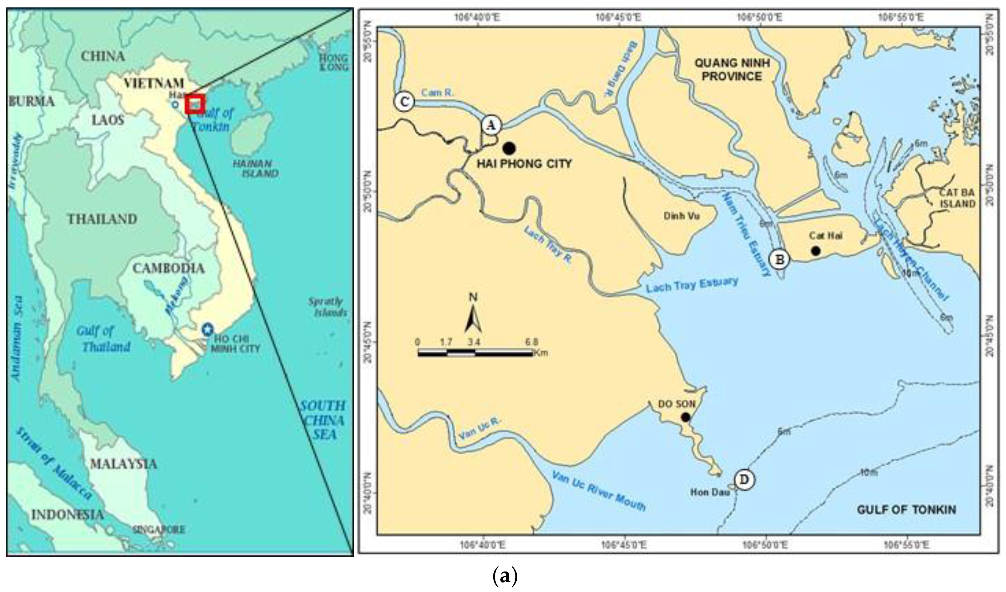
2. The Cam-Nam Trieu Estuary

The Cam-Nam Trieu estuary is located in Hai Phong city (the third largest city of Vietnam), northeastern of Vietnam (Figure 1a). This estuary receives water and sediment from the Cam River and the Bach Dang River. The present study is based on measurements performed along the Cam River estuary and in the Nam Trieu estuary, this area is hereafter referred as the Cam-Nam Trieu estuary.
The Cam River is one of two main distributaries (with the Van Uc river) of the Thai Binh River. Although the Cam and Bach Dang Rivers belong to the Thai Binh River, they also receive water and sediment from the Red River through the Duong River (see a map of connections within the Red River Delta in Vinh et al. [40]. The total river discharge through the Nam Trieu estuary to the coastal zone is about 20 × 109 m3 year−1, corresponding to 16.5% of the total water discharge from the Red-Thai Binh river system to the Tonkin Gulf [40].
Annually, sediment flux from the Red-Thai Binh River through the Cam and Bach Dang Rivers to the coastal zones was about 13.2 × 10⁶ t, until the Hoa Binh dam impoundment in the 1980s. From this period, a large amount of riverine sediment has been trapped in the reservoirs and the sediment flux through the Cam and Bach Dang Rivers to the coastal zones decreased to 6.0 × 10⁶ t year−1, in proportion to 17% the total sediment of the Red-Thai Binh River to the Red river coastal area [40].
The Cam-Nam Trieu estuary is under the influence of a tropical monsoon climate with alternation of dry winters and wet summers. Annual rainfall in the region (based on measurements at Hon Dau, 1978–2007) is 1161 mm, of which nearly 83% falls during the summer monsoon (May to October). The wind direction is dominantly (72.2%) from the East (NE, E, SE) and South (SW, S, SE) directions in summer (June to September), and from the North (NE, N, NW) and East (SE, E, NE) directions (92.1%) in dry season (December to March), from wind data measured at Hon Dau (1960–2011).
Located in the Red River system, the Cam and Bach Dang Rivers are strongly affected by its hydrological regime. Based on data from 1960 to 2010, the Red River discharge at Son Tay (near the apex of the Red River delta) varied from year to year over the range 80.5 (in 2010)–160.7 (in 1971) × 109 m3 year−1, with an average value of 110.0 × 10⁹ m3 year−1. Water river discharge encompasses strong seasonal variations, with 71–79% of annual total water discharge in the rainy season and only 9.4–18% during the dry season [40].
The Cam-Nam Trieu estuary is affected by tides which are mainly diurnal [41]. Based on the tide gauge measurements at Hon Dau station (1960–2011, Figure 1a), tidal amplitude is about 2.6–3.6 m in spring tide and about 0.5–1.0 m in neap tide.
Sediment sampling revealed a high percentage clay to fine silts in the Cam River (around station v41 on Figure 1) and a substrate more enriched in fine sand in the estuary (near v57 to v58) in 2008 [38].

3. Material and Methods
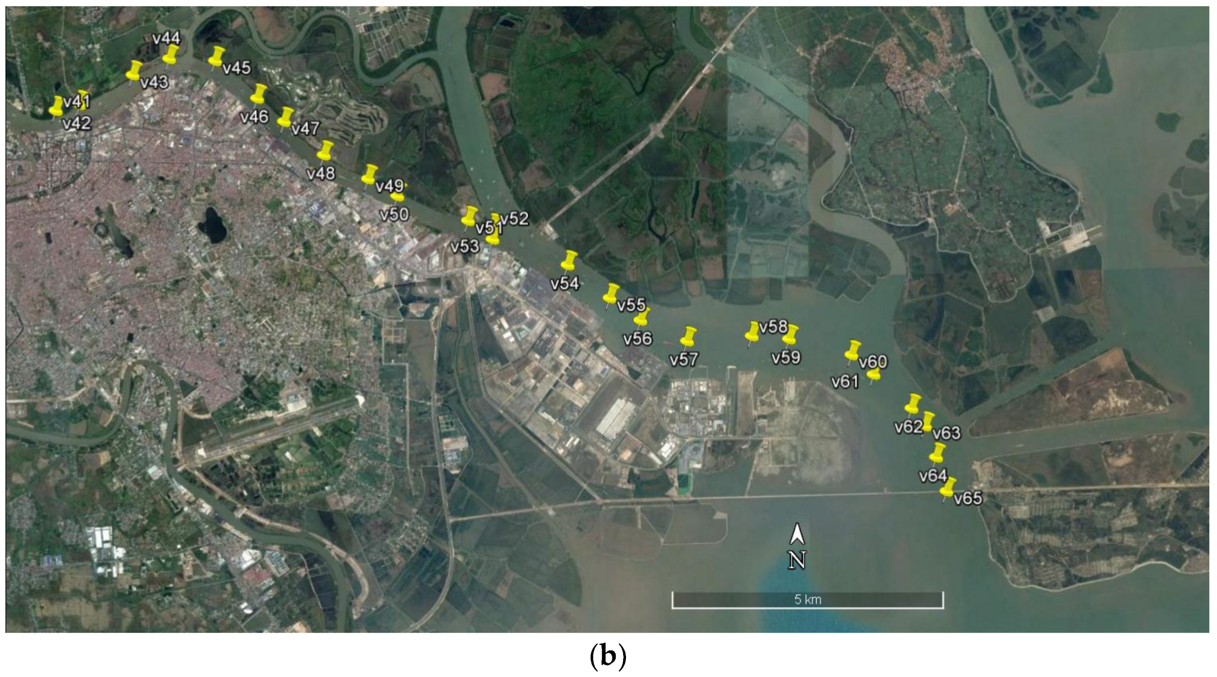
3.1. Field Data

A field survey was performed in the Cam-Nam Trieu estuary during spring tide from 10 May to 13 May 2015. Six along river transects from the upper estuary in the Cam River (position A, Figure 1a) to the Nam Trieu mouth (position B, Figure 1a) or the reverse were performed with a total of 110 stations (see one of the 6 transects on Figure 1b; a kml file is provided as Supplementary Material). At each station, velocity profiles were measured with a 600 kHz acoustic Doppler current profiler (ADCP RDI Workhorse in bottom tracking mode) configured for a 0.3 m bin size; depth profiles of water temperature, salinity and turbidity were measured by a Compact-CTD (ASTD687, Alec Electronics Co. (Nishinomiya, Japan), now released by JFE Advantech Co. (Nishinomiya, Japan) as Rinko-Profiler); depth profiles of floc size distribution and concentration were measured using an in situ laser scattering and transmissometry instrument with a 90% path reduction module (LISST-100X, Sequoia Scientific Inc. (Bellevue, WA, USA); e.g., [42,43]). The LISST of type B provided the volumetric particulate concentration in 32 logarithmically spaced size classes ranging from 1.25 to 250 μm and attenuation at λ = 660 nm. In order to study the relationship between turbidity and suspended particulate matter concentration, water samples were also collected using a Niskin bottle at each station 1.5 m below the surface. Turbidity of these samples were also measured onboard using a Hach 2100Q Turbidimeter.
The measurements did not show any influence of lateral inflow and outflow on turbidity along the transects, except near the new artificial straight channel at the North of Cat Hai island (near point B, Figure 1). This channel delivers clearer waters from the Halong Bay at some periods of the tidal cycle. We thus skipped 4 stations in this area when turbidity was affected by clearer waters from the analysis (v27 during Transect 2, v28 during transect 3, and v64-v65 during Transect 4, see Figure 1b).
Data at the hydrographic station of the Cam River (position C, Figure 1a), which were provided by the National Hydro-Meteorological Service (NHMS), are also used in this study. They include water river discharge (measured every hour) and SPM concentration (averaged values during flood tide and ebb tide). At the Hon Dau station in Hon Dau Island (position D, Figure 1), data include rainfall (daily), wind (every 6 h) and water elevation (every hour).

3.2. Data Processing

3.2.1. SPM Concentration and the Ratio Organic to Inorganic Matter in the Solids of Flocs

Suspended particulate matter concentration was determined by filtering about 100–150 mL per sample through pre-weighed polycarbonate Nuclepore filters (porosity 0.45 μm). Filters were rinsed three times with 5.0 mL of distilled water, dried for 24 h at 75 °C in an oven, and then stored in a desiccator until weighing on a high-precision electrobalance.
The same process was also applied at selected stations with GF/F filters (porosity 0.7 μm). The sediment concentration after drying at 75 °C provided the total SPM concentration, which includes organic and inorganic matter. After burning the filter at 450 °C during 2 h, all the organics had been removed and we measured the particulate inorganic matter (PIM) concentration. The difference between the total SPM and PIM provided the particulate organic matter (POM) concentration and thus the ratio of organic to inorganic matter within the solid part of the flocs POM/PIM.

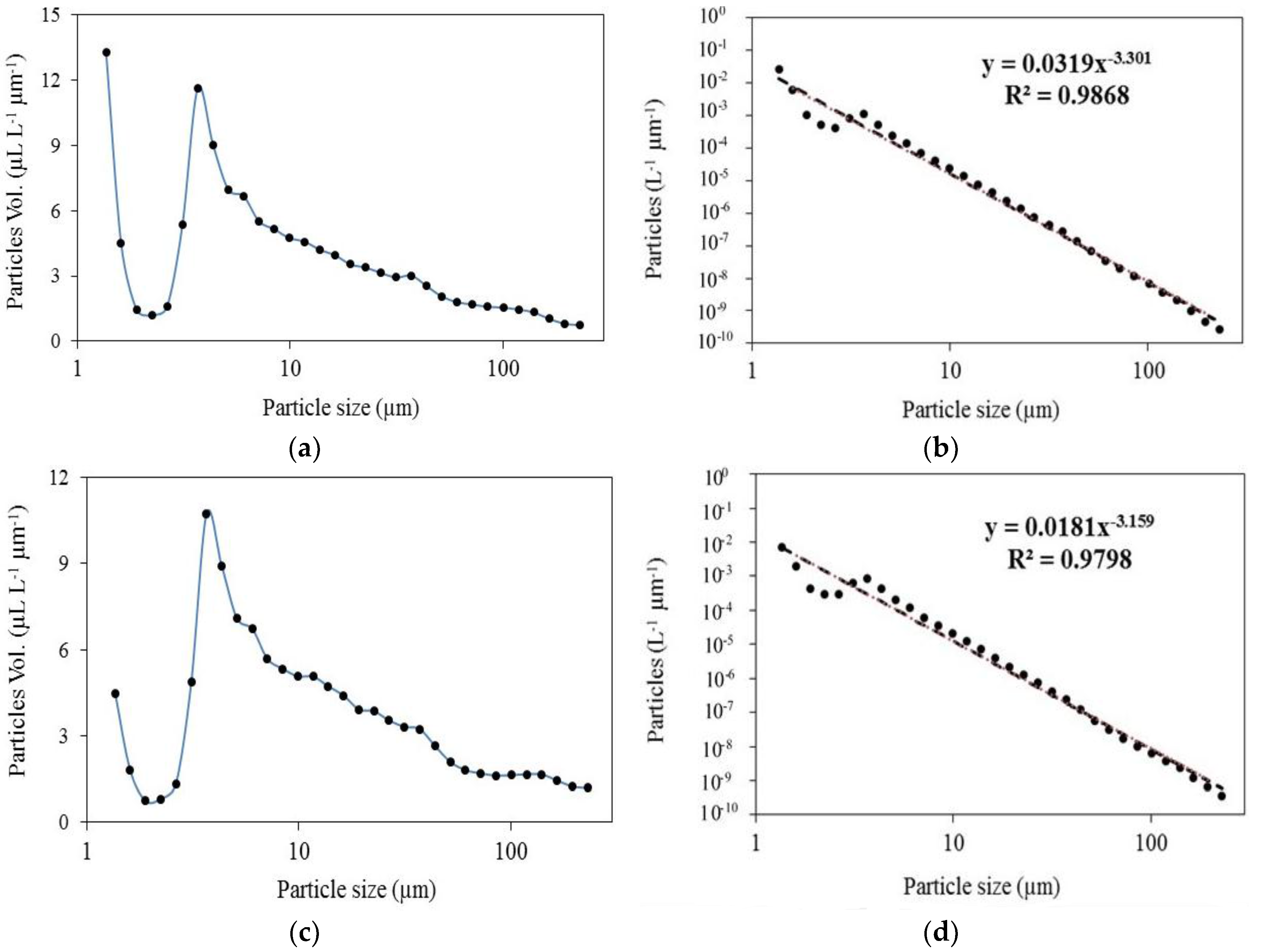
3.2.2. SPM Volume Concentration (SPMVC) and Particle Size Distribution (PSD)

The distribution of volume concentration of particles given by LISST-100X is discretized over the continuous spectrum of 32 size classes. Their sum is providing the SPM volume concentration (SPMVC). However, particles less than the smallest size class or bigger than the largest size class affect the measurements in the spectrum [42,43,44,45,46,47,48,49,50,51,52]. In this study, we followed the recommendation of former authors to remove the first and last classes for calculating the general slope of the particle size distribution and the mean apparent diameter D50 [42,43,44,45,46,47,48,49,50,51,52]. Based on data between class #2 and class #31, D50 was thus calculated as the diameter corresponding to 50% of the cumulative volume concentration of aggregates between 1.48 and 212 μm.
The number of particles of each class, N(D), was calculated from the volumetric particle size distribution (PSD) assuming spherical particles in the assemblage, after a normalization by the width of each logarithmically spaced size bin [47]. The more often, a power law relationship can be proposed between N and D following:
N ( D ) = a D j
where a is a coefficient (in number of particles L−1 µm−1), D is the diameter of aggregates and j is the dimensionless exponent, also referred to as the particle size distribution slope or the Junge parameter [53,54]. j provides information on the relative concentration of small to large particles: the steeper the slope, the greater proportion of smaller particles and the flatter the slope, the greater proportion of larger particles. Furthermore, j can be estimated from multispectral satellite data of ocean colour through the particulate beam attenuation [55] or the particulate backscattering coefficient [56,57]. For natural waters, j slopes generally vary from 3 to 5 with most values between 3.5 and 4 [58] and can be up to 7 for submicron particles in the ocean [57].
Due to the skip of the first class (<1.48 μm) and the last class (>212 μm) of the particle sizes, the remaining grain size range was analyzed through some groups: over the whole particle size range (1.48–212 μm), the fine particle size group (1.48–17.7 μm), the medium particle size group (17.7–92.6 μm), and the coarse particle size group (92.6–212 μm). The classes were defined from our measurements to separate the two extreme peaks (around 3.4 μm and 120–140 μm) from the intermediate peaks around 25 or 45 μm. Other groups may have been considered (e.g., [59]). The purpose of the groups here is only to illustrate the transfer of particles amongst them during the tidal cycle inferred by flocculation/disaggregation and/or sedimentation/erosion. The Junge parameter and aggregate settling velocity were also calculated for each of these 3 groups.

3.2.3. Excess of Density and Settling Velocity of Flocs

Settling velocity of flocs, ws, is the sinking velocity of a floc in still water, which may be reduced by the presence of other flocs that cause hindered settling [60,61,62]. In this study, ws was calculated from the Stokes formula [63]:
w s = 1 18 μ Δ ρ f g D 2
where µ is the dynamic viscosity of water, ∆ρf is the excess of density of flocs given by ∆ρf = ρfρ, ρ is the water density, ρf is the floc density and g the gravitational acceleration constant. The excess of density of flocs ∆ρf was either calculated at the points where the weight and volume suspended sediment concentrations have been measured, or estimated from the available data and the formulas proposed by Kranenburg [64] and Maggi [65].
At the stations where SPM, SPMVC and ρ were measured, ∆ρf was calculated under the assumption that flocs were made of particles (subscript p) and water (subscript w), and that their relative component of minerals and organic particles was known. In that case:
SPM SPMVC = M p V p + V w
where Mp is the mass concentration of flocs, determined from filtration, (Vp + Vw) is the volume of flocs measured by the LISST. If we note ω the ratio of particulate inorganic matter concentration (PIM, determined by loss of ignition of GF/F filters) to the particulate organic matter concentration (POM, determined as the difference between SPM and PIM), the density of the particulate component of flocs ρp was calculated following:
ρ p = M p V p = ω   ρ s + ( 1 ω ) ρ o
where ρs is the density of minerals in the flocs (hereafter considered to be 2650 kg m−3) and ρo is the density of organic matter (hereafter considered to be 1100 kg m−3, like in [66]). Finally, at this station, the measured excess of density was obtained by:
Δ ρ f = SPM SPMVC ( 1 ρ ρ p )
If SPM, ρ and ρp are expressed in g m−3 and SPMVC in µL L−1, ∆ρf is expressed in g mL−1 and must be multiplied by 1000 to provide a value in g L−1 (or kg m−3). This formula, combined with Equation (2), provided ws values from measurements.
Where SPM was not measured but inferred from turbidity, ∆ρf was alternatively estimated using the fractal description of flocs. Kranenburg [64] derived the excess floc density ∆ρf of a floc composed of primary particles of diameter Dp and density ρp, with fractal dimension df:
Δ ρ f = ( ρ p ρ ) ( D p D ) 3 d f
Maggi [65] adapted this formula to the case of a floc composed of mineral and organic particles with density ρs and ρ0, respectively, as follows:
Δ ρ f = [ ( ω ρ s + ( 1 ω ) ρ 0 ) ρ ] ( D p D ) 3 d f
which finally gives:
w s = 1 18 μ ( ω Δ ρ s + ( 1 ω ) Δ ρ 0 ) g D p 3 d f D d f 1
This formula was used to estimate the settling velocity of flocs [64,65,66,67]. In this study, it was applied with Dp = 4 µm (following Fettweis [68]: Dp = 1.1 µm in the ETM, 2.1 µm at the edge of ETM and 7.2 µm offshore), ρs = 2650 kg m−3 and ρ0 = 1100 kg m−3, like Maerz et al. [66] did, and df = 2 as suggested by Winterwerp [60]. Averaged values of ω amongst our measurements in May 2015 were considered for the applications (ω = 0.89 at flood tide, 0.85 at high and low tides, 0.91 at ebb tide).
A last point is studied regarding the settling velocity. From the settling velocity of one aggregate given by the Stokes relationship, Winterwerp [60] proposed a correction taking into account the turbulence generated by the flocs themselves in the water following:
w s c = w s 1 ( 1 + 0.15 R e p 0.68 )
where Rep = (ws D50 ρ)/μ. When Rep << 1, it comes wsc = ws. The correction factor was calculated for the 23 values of ws so as to estimate its potential influence in the Cam-Nam Trieu estuary.
Measured and modeled values of ws were compared using different statistics [69]: mean values and standard deviations for a given dataset, and mean normalized bias (MNB) and the normalized root mean square (rms) error, in percent, to compare variables obtained from a model and values measured in situ. MNB is an indicator of systematic error while rms is an indicator of random error. Slope, intercept and the coefficient of determination R2 were also calculated for the linear regression of estimations from Equation (7) versus Equation (5) for ∆ρf, and between ws estimations using Equation (8) or the Stokes formula combined with the measured ∆ρf. These statistics constitute a numerical index of model performance which can be compared to those of other models.

3.2.4. Richardson Number

The gradient Richardson number, Ri, has largely been used as a criterion for assessing the stability of stratified shear flow through energy consideration [70]. It is calculated from the data of ADCP and CTD, following:
R i = g ρ z ρ ( ( u z ) 2 + ( v z ) 2 )
where u, v are velocity components (m s−1) and ρ the local density of water including the sediment concentration.

3.2.5. Simpson Parameter

To quantitatively analyze the physical mechanisms contributing to mixing and stratification in an estuary, Simpson et al. [71] introduced the potential energy anomaly (Φ), which represents the mechanical energy (in J m−3) required to bring about complete mixing of the water column, given by:
Φ = 1 D H 0 g z ( ρ ¯ ρ ) d z
where ρ ¯ is the depth-mean density.

4. Results

4.1. River Discharge, SPM and Turbidity

The instant discharge of the Cam River at station C varies with the river discharge and is strongly impacted by the tidal oscillation. During the field survey (10–13 May 2015), the local and instant discharge varied between −1210 and 1490 m3 s−1 (negative values corresponding to a flow going upstream). The discharge often reached its maximum value 3–4 h before low tide and its minimum 2–3 h before high tide. The averaged values for each transect are given in Table 1. The values over one full tidal cycle (from low tide to the next low tide) were calculated per day and gave, in average over 3 days, 390 m3 s−1. They slightly increased from 299 m3 s−1 on 10 May to 460 m3 s−1 on 13 May. It must be noted that the average discharge at this station in May 2015 was 452 m3 s−1.
The average SPM concentration over the whole water column at the Cam hydrographic station C varied in the range 45–107 mg L−1 in ebb tide and 47.8–113.0 mg L−1 in flood tide. The suspended sediment flux was estimated using these values and provided an average discharge during the 4 days (10–13 May) of 25.4 × 10³ tons day−1. However, this value must be considered as a rough estimation only since it was calculated with only one “typical” value of SPM at ebb and another “typical” value during the flood tide, provided by the NHMS.
In the Cam-Nam Trieu estuary in May 2015, our measurements showed quasi-linear relationships between measured turbidity and SPM concentrations (Turb = 1.264 SPM + 18.30, N = 23, R2 = 0.971; or Turb = 1.392 SPM, N = 23, R2 = 0.957). Based on the relationship providing the best determination coefficient, SPM concentrations (mg L−1) were determined from the measured turbidity (FTU) profiles.
By definition, ETMs are estuarine areas where turbidity is the highest. During this survey in early flood period, turbidity of ETMs was generally found to be >200 FTU (approximately 140 mg L−1) in their core and ~150 FTU (approximately 100 mg L−1) at their edge.

4.2. Excess of Density of Flocs

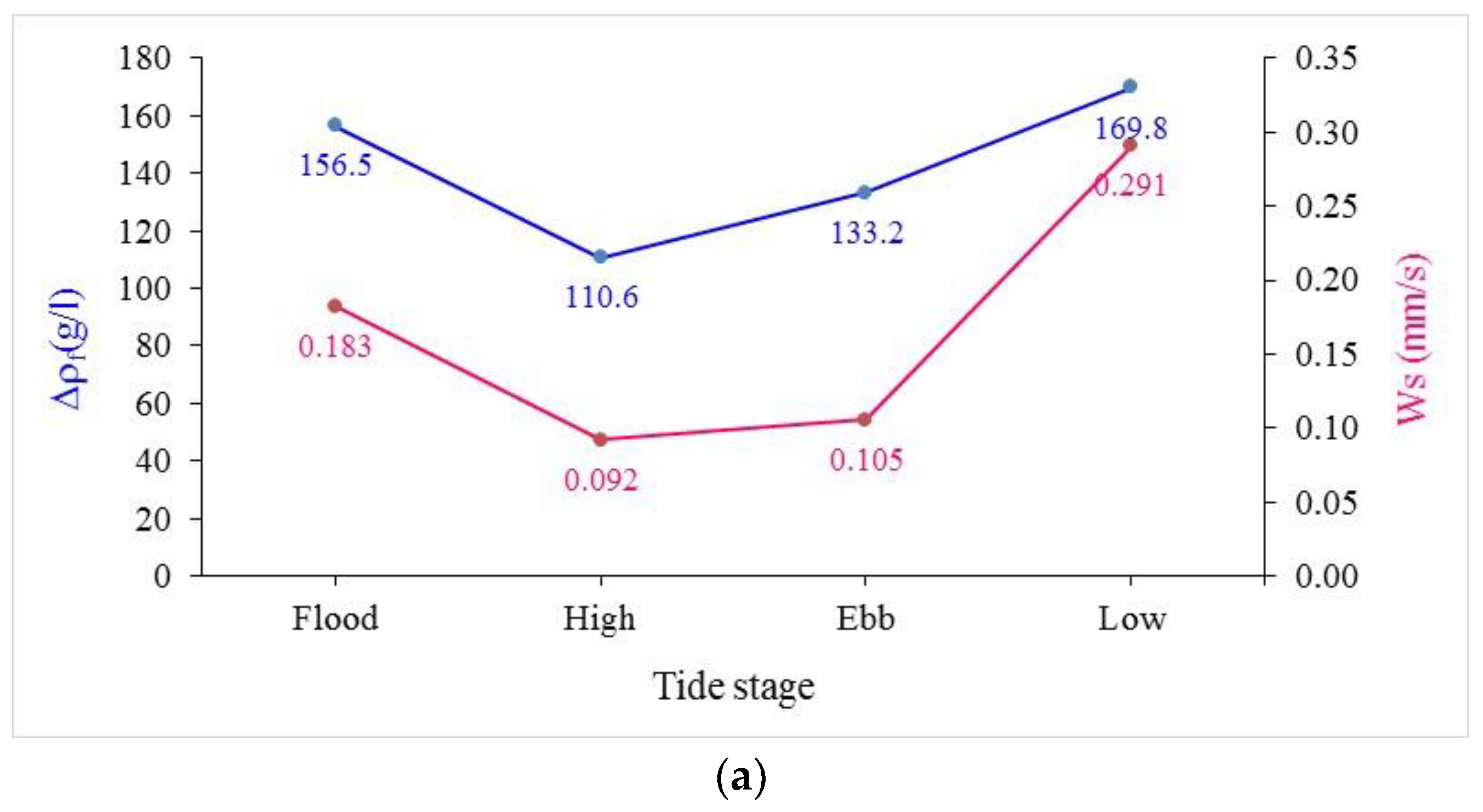
4.2.1. Tidal Variations of ∆ρf from Measurements

The average measured value of ∆ρf was 149 kg m−3 from the field data (SPMVC from LISST + SPM from weighting) over 23 stations. Its range was 66–260 kg m−3, yielding a factor of 3.9 between the highest and the lowest values. The corresponding settling velocity was in average ws = 0.184 mm s−1 from our measurements, with a range 0.07–0.46 mm s−1 expanded as compared to the one of ∆ρf (factor of 6.5).
If we compare separately the results for each tidal phase, we observe that ∆ρf was maximum at low tide (170 kg m−3), then decreased at flood tide (in average 156 kg m−3), reaching its lowest value at high tide (111 kg m−3), and increased again during ebb (133 kg m−3). ∆ρf was thus varying between 170 kg m−3 at low tide and 111 at high tide, its value being 53% higher at low tide than at high tide (Figure 2a).
The settling velocity was evolving in the same way. Around the average value of 0.184 mm s−1, we obtained the highest value at low tide (0.29 mm s−1), then 0.18 at flood tide, 0.09 at high tide and 0.11 at ebb. Similarly to ∆ρf, ws was varying between 0.291 mm s−1 at low tide and 0.092 mm s−1 at high tide (Figure 2a), its value being 3.1 times higher at low tide than at high tide.

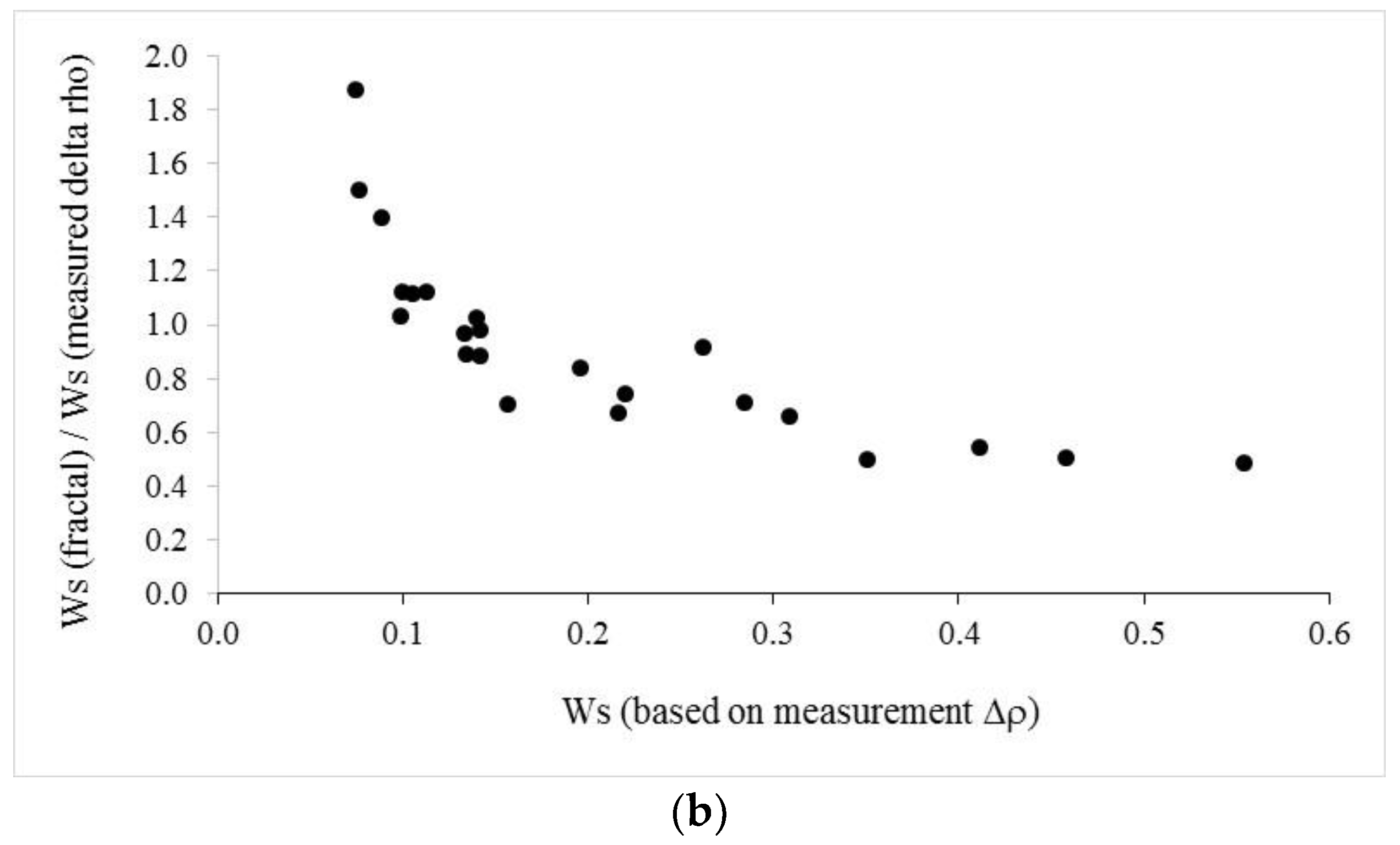
4.2.2. Comparison between Measured and Modelled Values of ∆ρf and ws

If we consider in a first approach that the Kranenburg formulation (Equation (6)) can be applied all along the tidal cycle with constant parameters (Dp = 4 µm and df = 2), we obtain in average over 23 stations (from high, low, ebb and flood tides), ∆ρf = 134 kg m−3—to be compared with the measured value of 149 kg m−3 from the field data. The mean normalized bias (MNB) is very small (+3.7%), the standard deviation is 32% and the mean quadratic error is 45.6 kg m−3.
Combining the resulting values of ∆ρf and the Stokes settling velocity formula, we obtained in average ws = 0.184 mm s−1 from our measurements and ws = 0.151 mm s−1 from the Equation (8), with the same MNB and standard deviation than ∆ρf, and with a mean quadratic error being worth 0.077 mm s−1.
Globally, the variables are thus rather close by the two methods. The comparison between both values for ∆ρf and ws are good. However, if we look in more detail the ratio ws-fractal/ws-measured ∆ρf versus ws-measured ∆ρf (Figure 2b), we observed that the fractal formula with constant parameters all along the tidal cycle tends to overestimate the smallest ws and underestimate the highest.
If we compare separately the results for each phase of the tidal cycle, we observe that the Equation (8) tends to underestimate ∆ρf and ws at low tide (MNB = −21.5%, N = 10), at flood tide (MNB = −13.9%, N = 7) and to overestimate them at ebb tide (MNB = +19.6%, N = 2) and at high tide (MNB = +37.9%, N = 4). As the individual particles should be the same at every tidal cycle (Dp unchanged), this result may suggest that df is changing along the tidal cycle around the mean value of 2. An estimation of df variations was performed so as to obtain the same ws values with Equation (8) and with the combined Equations (2) and (5). It gave averaged df values of 2.017 at flood tide, 1.968 at high tide, 1.984 at ebb tide and 2.038 at low tide.

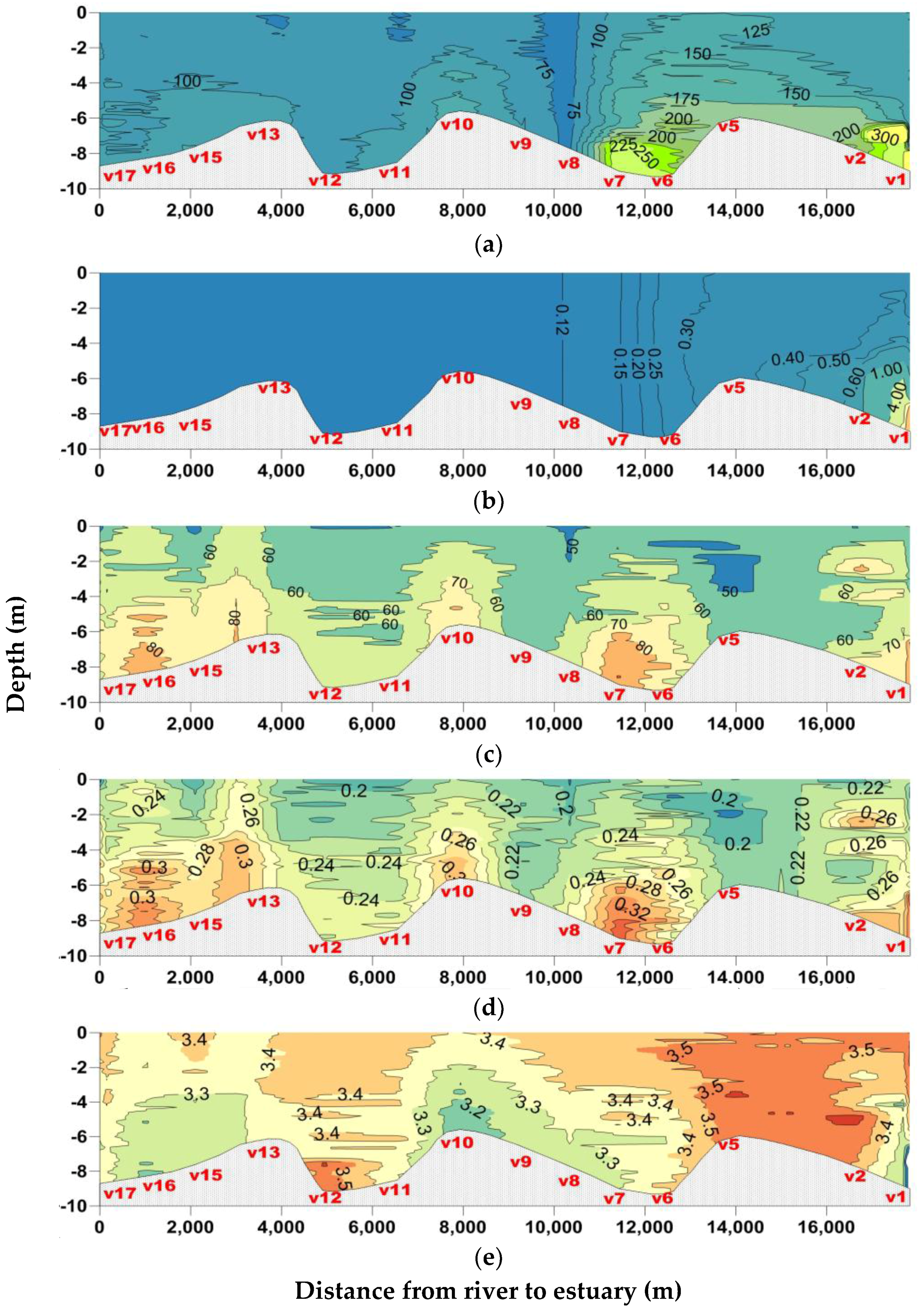
4.3. ETM Characteristics at Different Tidal Stages

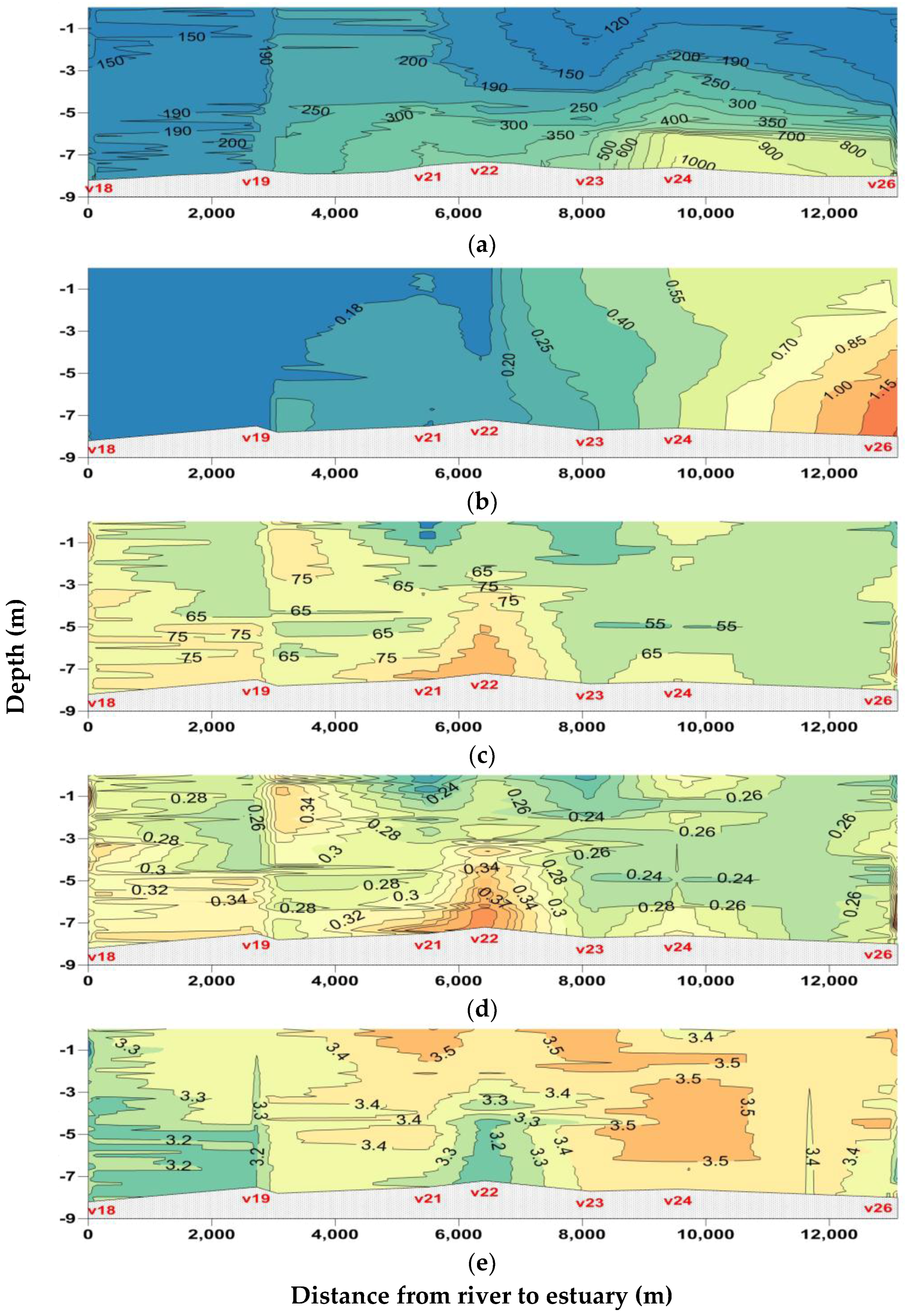
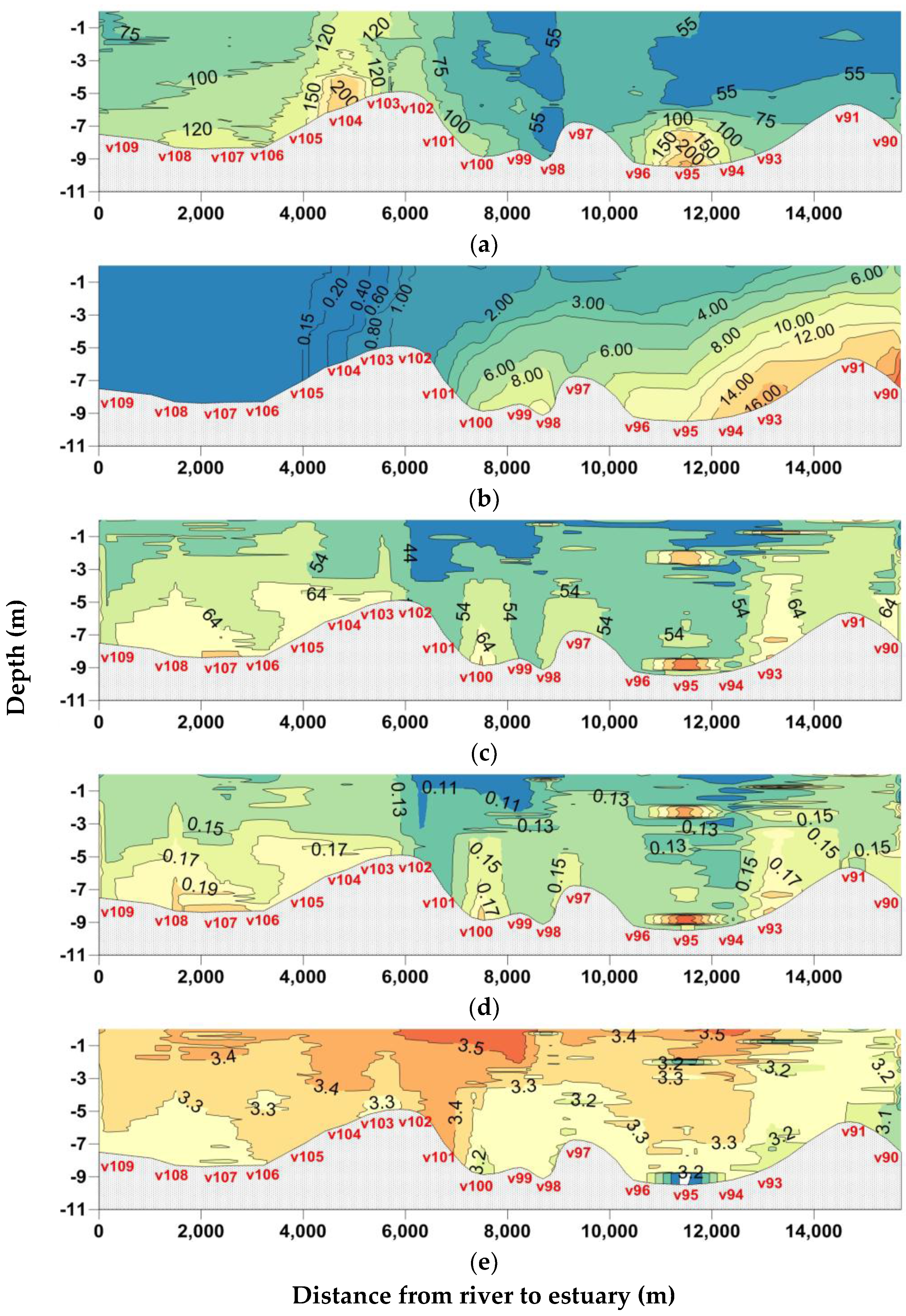
4.3.1. Transect 1–Flood Tide

The first transect was performed between stations v1 and v17 during flood tide (water elevation = 1.3–2.5 m), 10 May 2015. The longitudinal profile of turbidity showed a pronounced ETM located around v6-v7 stations (Figure 3a) with a maximum value above 250 FTU and another local maximum between v1 and v2 with a local turbidity >300 FTU. Salinity increased from the upper estuary (<0.1 psu) to the middle estuary (around 5 psu near bed at v1, Figure 3b and Table 2). This transect showed rather homogenous salinity profiles in the upper estuary until between v5 and v6, and a strong stratification downstream until v1.
The upper ETM (or upper part of the ETM) started at salinity ~0.13 psu between v8 and v7 and ends around v5 (~0.3 psu) (Figure 3b). Its length was around 3 km (Table 2). It developed over well mixed waters. The lower ETM developed over stratified waters at salinity higher than around 0.5–0.6 psu and was restricted to the bottom boundary layer (<4 m from the bottom). The whole upper ETM was sampled and measured, however, we likely measured and sampled only the upper part of the lower ETM at salinities between 0.5–0.6 psu, up to ~5 psu. The lower ETM was truncated by our measurements (region of salinity >5 psu was not sampled). While the longitudinal profile of turbidity near the bottom clearly exhibited two zones of maximum, only one turbidity maximum can be detected at the surface around station v5, in closer relation with the well mixed waters of the upper ETM than with the stratified lower ETM (Figure 3a).
D50 values over the whole size range (1.48–212 μm) varied between <50 μm and 90 μm (Figure 3c). Larger floc sizes (D50 > 70 μm) were observed near bottom between v13 and v17 and around v10 in the upper estuary, and in the cores of the two ETMs (between v6-v8 in the upper ETM and around v1-v2 in the lower ETM) (Figure 3c). The depth-averaged D50 was 71.7 μm at v6 in the upper ETM (Table 2), higher than the mean of whole transect (64.5 μm, Table 1). The same parameter was less than the average (62.9 μm) in the lower ETM but high variations were observed along the depth profile in the lower ETM, which much higher values near the bed in the core of the lower ETM than above. The D50 of fine (8.3 μm), medium (46.5 μm) and coarse aggregates (132.7) in the upper ETM (v6) were similar or higher than their average values along the whole transect (8.3 μm, 44.8 and 131.8 μm, respectively) or than in the lower ETM (8.1 μm, 45.0 μm and 131.3 μm, respectively) (Table 1 and Table 2). The smallest floc sizes (D50 ≈ 50 μm) were observed between v2 and v5, presumably due to floc disruption resulting from the shear at the salt wedge during flood tide.
Settling velocities of flocs ranged between 0.20 and 0.32 mm s−1 (Figure 3d), with an averaged value of 0.253 mm s−1 (Table 1). They were high (0.28–0.30 mm s−1) in some places of the upper estuary (v15 to v17, and v10), and at the edge of the lower ETM (v1-v2). Their highest values (0.28–0.32 mm s−1) were observed near bed in the core upper ETM (v6-v7), where the biggest flocs were observed. Aggregation process created bigger flocs and increased settling near the bed, thus enhancing turbidity in the ETM.
Particles of fine (1.48–17.7 μm), medium (17.77–92.6 μm), and coarse sizes (92.6–212 μm) along this transect occupied in average 22.3%, 35.2% and 41.5% of the volume concentration, respectively (Table 1). The median diameter of the finest class varied few around 8.2–8.4 μm values with a trend to a slight decrease along the transect. A higher value in the lower ETM was only visible at one station (v1) and thus could not be considered as representative. D50 of medium aggregates in this transect changed in the range 42–49 μm, with their highest values in the upper ETM (such as at v6, see Table 2). The longitudinal variations of D50 amongst the bigger aggregates were rather low, with a possible small increase around the upper ETM (D50 ≈ 132–134 μm).
Concerning the PSD, the number of particles per size class obtained with the LISST-100X showed a “tail” for the smallest size classes for which the slope is different than for the biggest particles, at most stations of all the transects. In the Cam–Nam Trieu estuary, these visible tails were observed for the particle size <3.98 μm (Figure 4). Above 3.98 μm, a power law relationship was fully effective and the logarithmic regression model fitted with the PSDs with R2 > 0.98. The values obtained over the full size range (1.48–212 μm) was kept in Figure 3 and Tables for a better comparison with other sites. In the first transect, the PSD slope showed slight variations within the estuary, around the averaged value of 3.37 (Table 1). j was seen to be lower where D50 was the highest, in the upper estuary, at the edge of the upper ETM and in the lower ETM (3.34 in average at v1, see Table 2; locally <3.2, see Figure 3d). Vertical distributions showed lower values of j near the bottom.
The Simpson parameter Φ was calculated at each station. Its value was <1 from upstream until station v6 (included, with Φ = 0.98), since the water column was rather homogeneous in density. Its value was >1 at stations v2 and v1 in the lower ETM, with a value = 2.6 at v2 and 57.1 at v1 (Table 2).
The average Ri in the upper estuary (between v17 and v7) was 0.26, indicating stable conditions. Meanwhile, averaged Ri in the lower part of the estuary (v6 to v1, where the ETM was located) was 0.13 (Table 2).

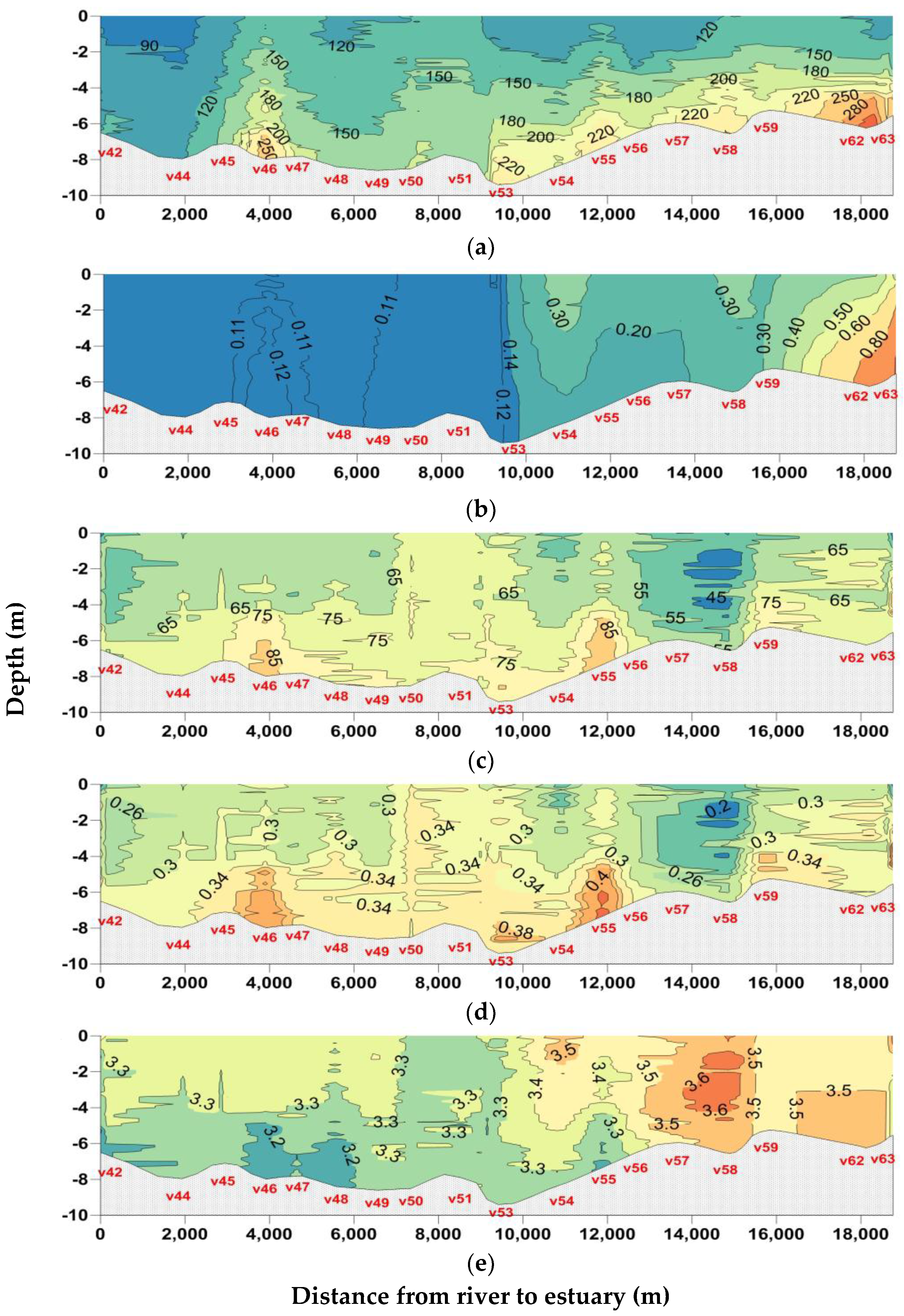
4.3.2. Transect 2–Low Tide

The transect 2 was measured at low tide (water elevation below 0.7 m), 11 May 2015. The longitudinal profile was interpolated from measurements at stations v18 to v26. An upper ETM can be seen from v18-v19 (salinity ~0.15 psu) up to v22 (salinity~0.20–0.25 psu) in well mixed waters with maximum turbidity >350 FTU (Figure 5a,b); it was visible from the bottom to the surface. A lower ETM with much higher turbidity values (up to more than 1000 FTU) developed from v23-v24 to v26 at salinity between 0.4 psu and ~1.2 psu (Table 2), where the flow from well mixed changed to become stratified (Figure 5a,b); this lower ETM was restricted to the bottom boundary layer at heights <4 m from the bottom. V24 was located at a distance about 10 km from the station A in the river (Figure 1). Like during the transect 1, the transition between the upper and lower ETMs was not abrupt, we can only observe a transitional area with a local turbidity which is slightly lower between both ETMs. Each measured ETM was around 4–5 km in length.
Floc sizes profile distribution showed a trend of D50 to decrease from the upper estuary to its lower part with typical change from 65–75 μm to 55–65 μm (Figure 5c). The largest flocs were measured near bed between v21 and v22 (D50 up to 85 μm), and were associated with locally reduced turbidity under 4 m below the surface. Meanwhile, floc sizes in the core of the lower ETM (v24 to v26) were smaller (D50 = 55–75 μm). D50 showed its smallest values in the upper ETM (65.5 μm, less than the average over the whole transect 2: 72.2 μm, Table 1) and in the lower ETM (56.8 μm, Table 2). In the upper ETM, D50 of the fine aggregates (8.5 μm, Table 2) was higher than the average over the whole transect (8.4) or the lower ETM (7.8), but D50 of the medium and coarse aggregates (46.4 μm and 130.9 μm, respectively) were slightly less than their average values over the whole transect (47.9 μm and 131.0 μm) and in the lower ETM (47.7 μm and 136.1 μm) (Table 1 and Table 2). This may indicate that D50 increased upstream for the finest aggregates in the upper ETM, then downstream for the coarser particles in the lower ETM.
Settling velocity of flocs ranged from 0.22 to 0.37 mm s−1 (Figure 5d). The average of the whole transect was 0.316 mm s−1 (Table 2). The highest values were observed in the upper estuary (v18-v19: 0.30–0.34 mm s−1), in the core of the upper ETM (v21-v23: 0.30–0.37 mm s−1), and at the upper edge of the lower ETM (v24: up to 0.30 mm s−1). The settling flocs in other regions varied from 0.22 to 0.28 mm s−1. The settling velocity of flocs varied between 0.28 and 0.36 mm s−1 in the upper ETM (Figure 5d) and was slightly higher than in the lower ETM (Figure 5d).
The floc sizes ratios showed that fine, medium and coarse aggregates occupied in average 18.9%, 37.5% and 43.6% of the volume concentration, respectively (Table 1). As compared to the flood tide of transect 1, they likely show a transfer from fine to medium and from medium to coarse particles, between flood tide and low tide.
The longitudinal distribution of the finest aggregates showed mostly a trend to decreasing from the upper (D50 = 9.1 μm) to the lower part of the estuary (D50 = 8.5 μm). Their median diameter was seen to be the smallest in the core of the lower ETM (around v24, in the range 7.8–8.1 μm from near bed to the surface). Bigger floc size (D50 ~8.7–9.1 μm) was observed at the edge of the lower ETM, around v23. The medium aggregates size showed high variations along transect and increased between the upper and the lower ETM. Their highest value (~52 μm) was located around station v22 at the lower edge of the upper ETM, and under 3 m from surface. From each side of this maximum, the median size of medium aggregates fell down to 46 μm. The coarser aggregates were the biggest in the core of the lower ETM (around v24), with D50 being worth 130–133 μm near bed and 134–136 μm below the surface. Opposite vertical variations were observed in the core of the lower ETM (v24) with the fine and medium aggregates whose size was higher near bed. This showed a transfer to coarser aggregates around v24 which settle faster and which likely explain the presence of very high turbidity in the bottom boundary layer of the lower ETM. The median diameter of the coarser aggregates was also seen bigger in the upper ETM (from v19 to v22) than upstream and downstream (i.e., between both ETMs). D50 of the finest and medium aggregates clearly decreased in the upper edge of the upper ETM, where D50 of the coarser particles increased. D50 of the medium particles increased in the core of the upper ETM.
The PSD slope, j, slightly increased from upstream (~3.2) downwards, until 3.4–3.5 around the lower ETM. j was higher in the upper ETM (3.54) and in the lower ETM (3.43, Table 2) than its average value (3.36) along the transect (Table 1).
PSD slopes were lower (<3.2) in region with higher settling velocity (>0.32 mm s−1, e.g., v22 or between v18 and v19), and higher (>3.4) in region with settling velocity of floc less than 0.28 mm s−1 (Figure 5d,e).
The Simpson parameter Φ value was <1 from upstream up to v22 then increased with the stratification in salinity (until Φ = 4.68 at v26). Its value was 0.97 in the upper ETM (at v21) and 1.22 in the lower ETM at v24 (Table 2).
The average Richardson gradient number was small upstream (0.05 at v18 and v19) then slightly increased downwards to 0.07 in the upper ETM (between v20 and v24) and 0.11 in the lower ETM area (between v24 to v26) (Table 2).

4.3.3. Transect 3–Flood Tide

The third transect includes data of stations v29 to v41, measured during flood tide (water elevation = 1.3–2.4 m), 11 May 2015. The salinity strongly changed along this transect at flood tide from less than 0.11 psu in the upper estuary to 12 psu in the lower estuary (Figure 6b). The measurements showed two ETMs (Figure 6). A smaller and upper ETM was observed between v38 (salinity ≈ 0.11–0.12 psu) and v35 (salinity ≈ 0.15 psu) with a maximum turbidity above 450 FTU and a length of 3 km. It developed from the bottom until around 2/3 of the water column, over well mixed waters (Figure 6a). A lower ETM started around v34 (salinity ≈ 0.25 psu) and ended at v29 (salinity ≈ 10–12 psu), its length being about 6 km (Table 2). Turbidity in the lower ETM increased from 150 FTU (at v34) until 900 FTU (at v29) near the bottom. The lower ETM developed mainly at 2–4 m above the bed over stratified waters and turbidity was seen to highly increase for salinity >1 psu, until 10–12 psu (Figure 6b).
D50 varied between 40 and 70 μm, with an average value of 51.4 μm (Figure 6c, Table 1). Its highest values (>60 μm) were observed near the bed, upstream (v38-v40), between the two ETMs (v34-v35) and in the lower ETM (between v29 and v31) (Figure 6c). Its depth-averaged values were smaller in the upper ETM (45.8 μm) and in the lower ETM (50.9 μm, Table 2) than the average value over the full transect.
The settling velocities of flocs were relatively small with values in the range 0.14–0.26 mm s−1 (Figure 6d). Their spatial variations followed the one of D50 (Figure 6c). Its depth-average value in the upper ETM (0.15 mm s−1 at v37, Table 2) and in the lower ETM (0.17 mm s−1 at v30) were less than the average over the whole transect (0.172 mm s−1, Table 1). In the core of the upper ETM (v37), flocs settling velocities were 0.14–0.18 mm s−1, and slightly higher in the core of the lower ETM (v30).
The fine, medium and coarse particles occupied 28.3%, 36.0% and 35.7% of the particle volume concentration, respectively (Table 1), with more fine particles and less coarse particles that during the transect 1, also performed during the flood tide. Amongst the six transects, this one showed the highest percentage of fine flocs and the second lowest percentage of coarse flocs (Table 1). D50 of the finer particles was higher in the upper ETM (8.0 μm at v37, Table 2) and in the lower ETM (8.4 μm) than in average (7.9, Table 1). D50 of the medium floc size was seen to locally increase at the edges of the lower ETM. The highest D50 for the coarser aggregates (131–135 μm) were observed at v31, in the core of the lower ETM. These values may result from a transfer of small and medium aggregates to bigger particles from downstream to upstream (v29 to v31), which settled and formed the core of the lower ETM.
The average j value was 3.55 (Table 1), with local values higher in the upper ETM (3.74 at v37, Table 2) and smaller in the lower ETM (3.48 at v30). Its highest values were seen in the core of upper ETM and at the edge of the lower ETM (v32, Figure 6e).
The Simpson parameter Φ value was <1 from upstream up to v33 except at v37 (1.86) in the upper ETM. Then its value increased with the stratification in salinity: Φ = 1.83 at v32 at the edge of the lower ETM, 29 at v31 and 87 at v30 in the lower ETM (Table 2).
The average Richardson gradient number increased seaward: 0.01 in the upper estuary (between v41 and v38), 0.05 between v38 and v34 around the upper ETM, and 0.28 in the lower ETM (Table 2).

4.3.4. Transect 4–Low Tide

The transect 4 was performed during low tide (water elevation = 0.7–0.8 m, 12 May 2015), from station v42 to v63 (Figure 7). Salinity on the longitudinal profile showed homogeneous depth-profiles in the upper estuary (from v42 to v53) until 0.14 psu. Salinity increased to 0.8 psu in the lower ETM and was highly stratified from v59 downwards (Figure 7b). The measurements showed two zones of maximum turbidity within the 15-km long turbid estuarine zone which extended from v45 (salinity ≈ 0.11 psu) to v63 where salinity >0.8 psu. An upper ETM (6-km in length) was observed from the bottom to the surface in the well mixed waters with salinity between 0.11 and 0.14 psu (v53), while a lower and stratified ETM developed at higher salinity (Figure 7a,b). The upper boundary of the lower ETM is difficult to determine precisely but it is clear that the maximum of turbidity (>300 FTU) was measured around stations v62-v63 near the bottom at salinity ranging between 0.8 and 1 psu. The lower ETM likely developed further downstream at higher salinity but this region was not investigated during the survey.
D50 of the full range of floc grain sizes was similar than in the transect 2 also at low tide, much higher than those at flood tides (transects 1 & 3), with an averaged value of 69.4 μm (Table 1). D50 was much higher in the upper ETM (78.6 μm at v46, Table 2) than in the lower ETM (64.2 μm). D50 was the highest (>75 μm) near the bed in the upper ETM (v46) and between the cores of the two ETMs at salinity 0.16–0.18 psu (v54-v56). It decreased further downstream in the region of salinity 0.20–0.40 psu (between v57-v59, Figure 7c).
Settling velocities varied accordingly, in the range 0.2–0.4 mm s−1, with its highest values where D50 was the biggest in the core of the upper ETM (around v46, 0.3–0.4 mm s−1) and between the two ETMs (around v55) (Figure 7d). Its lowest values were observed just downstream (0.2–0.28 mm s−1 at v57-v58).
The fine, medium and coarse particles occupied 20.2%, 37.6% and 42.2% of the volume concentration, respectively (Table 1), in very close proportion to transect 2 also performed at low tide. It clearly shows that the percentage of the smallest particles is at minimum and the one of the coarse particles is maximum during low tide. The distribution of the fine floc size along transect showed D50 decreasing from the upper part of the estuary (8.9 μm) to the river mouth (8.1 μm), with higher values in the upper ETM (8.7–8.9 μm, v46) than in the core of the lower ETM (8.1–8.5 μm). The fine aggregates were the smallest (D50 < 8.1 μm) in the surface layer above the lower ETM. D50 of the medium aggregates were higher in the salinity range 0.10–0.18 psu in the upper ETM and adjacent mixed waters, and in the lower ETM at salinity >0.35 psu. D50 of the coarse aggregates showed 3 zones of higher values along the transect: near bed in the upper ETM (v46), between the two ETMs (v54-v56), and at the upper edge of the lower ETM (v59), where the D50 values calculated over the full size range was also the highest (Figure 7c). The resulting variations are consistent with those one observed during transect 2 with bigger fine aggregates in the upper ETM, bigger medium aggregates at salinity around 0.18 psu and bigger coarse aggregates at the upper edge of the lower ETM.
D50 of fine (8.5 μm), medium (48.8 μm) and coarse aggregates (133.1 μm) in the upper ETM were higher than their average values over the whole transect (8.4 μm, 47.0 μm and 131.7 μm, respectively, see Table 1). Otherwise, we observed D50 values less than the average for the finer and medium flocs (7.9 μm and 46.9 μm) and higher than the average for the coarse aggregates (to 133.5 μm) in the lower ETM (Table 2). As a result, the settling velocity of flocs was higher in the upper ETM (0.38 mm s−1) than in the lower ETM (0.31 mm s−1, Table 1) and in average over the whole transect (0.33 mm s−1, Table 1) (Figure 7d).
The PSD slope in this transect was 3.37 in average (Table 1) and was smaller in the upper ETM (3.27 at v46, Table 2) than in the lower ETM (3.55 at v62). The PSD slope was generally less near the bottom (~3.2–3.3) than below the surface (~3.3–3.5), and in the upper estuary (~3.2–3.3) than further downstream (~3.5–3.6). These results also confirmed again the close co-evolution of ws and j (Figure 7d,e).
The Simpson parameter Φ was <1 everywhere except at v62 (3.06) and v63 (1.79). Its value was 0.74 at v46 in the upper ETM (Table 2). Ri increased downwards, from 0.04 in the upper estuary (between v42 and v53) to 0.06 between v53 and v59, until 0.19 in the core of the lower ETM (Table 2).

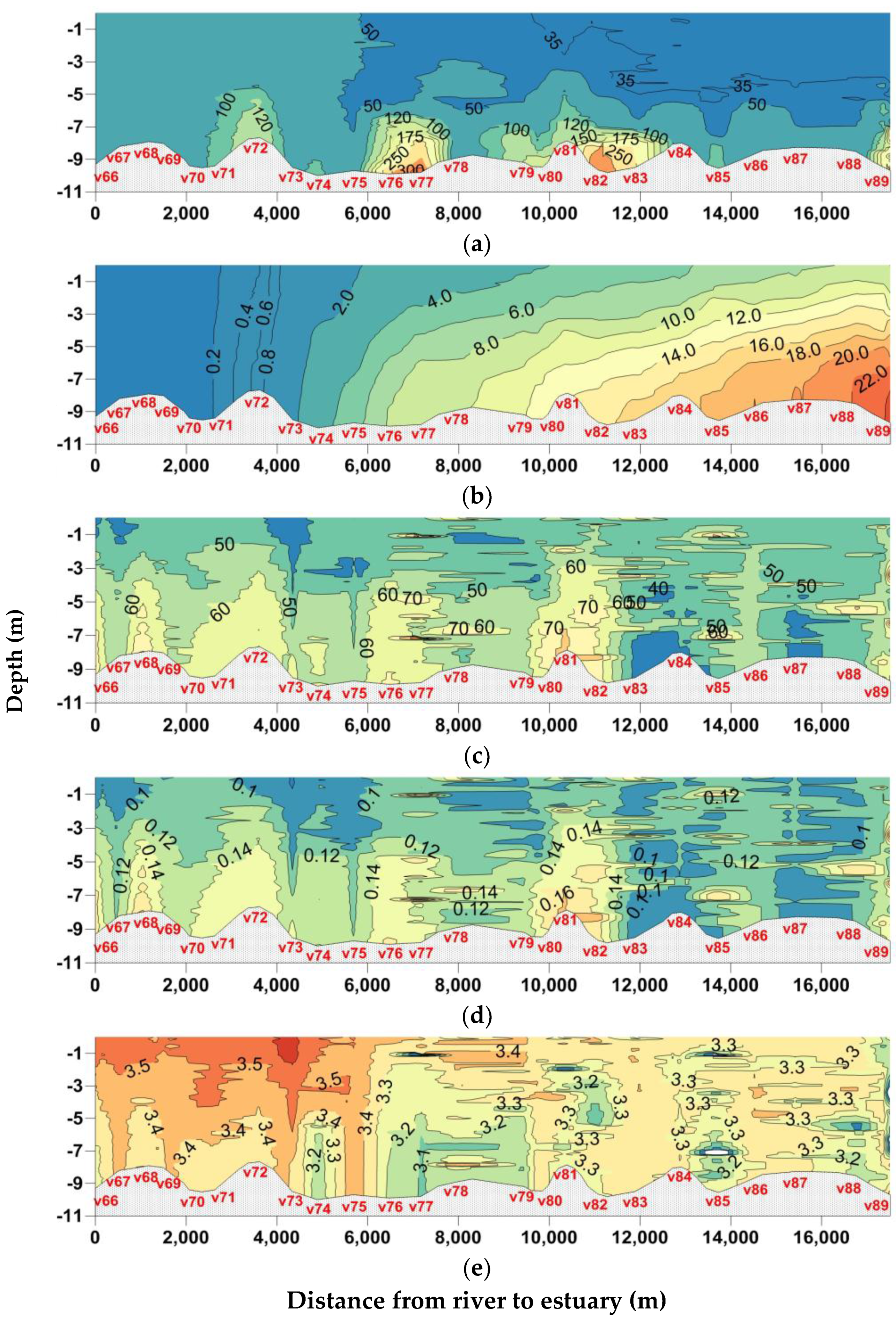
4.3.5. Transect 5–High Tide

The transect 5 was performed from stations v66 to v89 during high tide (water elevation = 2.5–2.7 m, 12 May 2015). The salinity range measured in the estuary was much larger than during flood or low tides, up to 24 psu. Salinity profile at high tide showed 3 parts: homogeneous waters at salinity <0.2 psu in the upper estuary (between v66 to v71), a transition zone around v72 and v73, then a strong stratification in the lower estuary at salinity >2 psu (between v73 to v89, Figure 8b). Two main turbid structures can be observed in the estuary with distinct characteristics from the previous configurations (Figure 8a). An upper ETM 4-km in length was observed in well mixed waters from salinity 0.11 psu (v66) up to ~1 psu (v72-v73) (Figure 8b). A lower ETM 6-km long was observed in the bottom layer of stratified waters at salinity between around 5 psu (v75) and 15 psu (v83). Their turbidity maxima were lower than during low tide and flood tide, of the order 130 FTU in the upper ETM and locally 300 FTU in the lower ETM (Figure 8a). The lower ETM was restricted to a 2-m high boundary layer, turbidity in the surface layer being <50 FTU.
D50 calculated over the full size range varied largely from less than 40 to 80 μm, the average values being 51.1 μm (Table 1, Figure 8c). D50 values decreased near the bed from the upper estuary (D50 > 60 μm) to the lower estuary (D50 < 50 μm), with higher values in the ETM (60–80 μm at v72, v76-v77, v81-v82). However, its values were lower in the upper ETM (54.2 μm at v72) than in the lower ETM (62.1 μm at v82, Table 2). The measurements also showed that D50 in the 5-m thick surface layer was generally less than 50 μm (Figure 8c).
The settling velocities of flocs at high tide were small and varied in a large range, between 0.10 and 0.16 mm s−1 (Figure 8d), in close relationship with D50 variations. Their highest values were observed in the upper ETM (at v68 and v72) and at the two edges of the lower ETL (0.12–0.14 mm s−1 around v76-v77 and 0.12–0.16 mm s−1 around v81-v82). The settling velocity of flocs were lower (<0.12 mm s−1) further downstream.
The fine, medium and coarse particles occupied 27.9%, 35.7% and 36.4% of the volume concentration, respectively (Table 1). It corresponds to the highest proportion in small aggregates amongst the six transects. The biggest aggregates in the small fraction were observed in the lower ETM (D50 up to 8.9 μm), while they were <8 μm in the upper estuary (Table 2). D50 of the medium size flocs were higher in both ETMs (D50 ~42 μm) than elsewhere (41 μm in average, Table 1). The bigger aggregates of the coarse fraction (D50 > 137 μm) were observed over the highly stratified station v81 at salinity ranging from 7 to 14 psu in the lower ETM (Figure 8b). Another local maximum (>134 μm) was observed in the upper ETM.
D50 of fine (7.7 μm) and coarse aggregates (133.7 μm) in the upper ETM were less than their average values over the whole transect (8.2 μm and 134.3 μm, respectively, Table 1) and in the lower ETM (8.5 μm and 136.8 μm, respectively, Table 2). Otherwise, D50 of medium size aggregates in the upper ETM (43.0 μm) was higher than in the lower ETM (41.5 μm) and in average (41.0 μm, Table 2). As a result, the settling velocities of flocs were smaller in the upper ETM (0.12 mm s−1 at v72) than in the lower ETM (0.14 mm s−1 at v82, Table 2). Both values were higher than their average along the whole transect (0.116 mm s−1, Table 1).
The PSD slope was 3.37 in average (Table 1, Figure 8e). It decreased from the upper estuary (3.4–3.5) to downstream (3.2–3.3), differently than at flood and low tides. J was higher in the upper ETM (3.55 at v72) than in the lower ETM (3.25 at v82, Table 2).
This high stratification at high tide induced very high values of Φ downstream. While Φ remained <1 from v66 to v71 (thus including a part of the upper ETM), it highly increased to 2.05 at v72, 4.79 at v73 and between 12 and 90 downstream. Its typical values were amongst the highest within the 6 transects in both ETMs (Table 2).
The average Ri increased from 0.04 in the upper estuary (between v66 and v71) to 0.2 in the upper ETM (v72), then to 1.53 at the lower edge of the lower ETM (v82) and to 1.86 downstream, between v84 and v89 (Table 2). The lower estuary was thus highly stable.

4.3.6. Transect 6–Ebb Tide

The transect 6 was performed from station v90 to v109 during ebb tide (water elevation = 1.5–2.4 m, 13 May 2015). The distribution of salinity was similar than transect 5 but the upper estuary extended further seaward: homogeneous salinity was observed in the upper estuary (S < 0.15 psu between v105 and v109), then a transition zone was seen for salinity between 0.15 and 1 psu (between v105 and v102) and a strong stratification was measured in the lower estuary (2–18 psu between v102 to v90, Figure 9b). The transect 6 clearly showed two ETMs along the estuary. A 2-km long upper ETM developed over well mixed waters between salinity 0.12 psu at v105 and 0.8 psu at v103 and can be detected at the surface (Figure 9a,b). A shorter (1.5-km long) and lower ETM developed over stratified waters in the bottom boundary layer at salinity between 8 and 15 psu. Although the core of both ETMs (turbidity >200 FTU) had almost the same size, the edge of the upper ETM was larger than the edge of the lower ETM. Turbidity in the surface layer above the lower ETM was around 50 FTU or less (Figure 9a). The configuration was similar to the one during high tide (transect 5) but with much shorter extent at ebb tide than at high tide.
D50 values varied between 40 and 80 μm. High values were measured near the bed in the core of the upper ETM (>64 μm, v103-v105) and in the core of the lower ETM (up to 80 μm at v95). Small values were observed in the surface layer of the transition zone and of the stratified region (D50 < 50 μm below the surface from v102 to v93, Figure 9c). Contrary to the transect 5, the depth-averaged values of D50 were lower in the upper ETM (57.1 μm, Table 2) and in the lower ETM (55.6 μm) than their average value over the whole transect (52.8 μm, Table 1).
The settling velocities of flocs varied between 0.10 and 0.21 mm s−1, with higher values near the bed, this being reinforced in the two ETMs (Figure 9d). The lowest settling velocities (<0.15 mm s−1) were observed in the surface layer of the transition and stratified waters. Like for D50, the depth-profile of ws showed high variations due to irregular aggregation in this area.
The fine, medium and coarse particles occupied 25.8%, 38.8% and 35.4% of the volume concentration of suspended particles, respectively (Table 1). This corresponds to the maximum of medium aggregates and to the minimum of coarse aggregates amongst the 6 transects (Table 1). The highest D50 of the fine fraction was observed in the core of the lower and stratified ETM at ~15 psu salinity (up to 9 μm at v94-v95), and at salinity 2–3 psu around station v101 over the whole water column. D50 of the medium fraction varied between 40 and 47 μm, the highest values being observed in the upper ETM around 0.15 psu waters and the smallest at salinities between 3 and 15 psu (from v93 to v99). D50 of the coarser aggregates was the highest (D50 = 133–136 μm) at the edges of the lower ETM (around v94 and v96), and much lower in the upper ETM. In summary, the lower ETM was characterized by bigger fine and coarse aggregates, while larger medium aggregates were observed in the upper ETM (Table 2).
The settling velocities of flocs were slightly higher in the upper ETM (0.16 mm s−1) than in the lower ETM (0.15 mm s−1, Table 2) (Figure 9d). They were slightly higher in both ETMs than the average of whole transect (0.141 mm s−1, Table 1).
The PSD slope was 3.38 in average (Table 1) and was globally decreasing from upstream (3.3–3.4 in the upper estuary) to downstream (3.1–3.2 at the river mouth), indicating the increasing proportion of coarser particles seaward (Figure 9e). It was thus higher in the upper ETM (3.40 at v104, Table 2) than in the lower ETM (3.36 at v95). Again, the PSD slope patterns showed a close relationship with the settling velocity of flocs (Figure 9d,e).
While the Simpson parameter Φ remained <1 until v105 (at the edge of the upper ETM), its value increased to around 1.6 in the upper ETM (Table 2) and had values >6 at v101 downwards. Its value was around 70 in the lower ETM (Table 2).
The average gradient Richardson number increased from 0.02 in the upper estuary (between v105 and v109) to 0.23 in the upper ETM (between v102 and v105, Table 2), 1.16 in the lower ETM (at v95, Table 2) and 1.34 downstream (between v102 to v 90).

5. Discussion and Conclusions

5.1. Q, Qs and SPM in Early Flood Season

The river discharge measured at the Cam hydrologic station (390 m3 s−1 in average from 10 to 13 May 2015) was typical of intermediate discharge between values measured in the Cam River in dry season (181 m3 s−1) and in wet season (806 m3 s−1) in 2008 and 2009 [38]. It corresponded to a period of increasing rain over the water basin and we noted a short flood during the three days of measurements, while Q changed from 299 m3 s−1 on 10 May to 460 m3 s−1 on 13 May 2015.
The solid discharge estimated from the data at the hydrologic station (Qs = 25.4 × 10³ t day−1) seems high as compared to the measured values in 2008–2009 (1.2 × 10³ t day−1 in dry season and 18.3 × 10³ t day−1 in wet season). However, this estimate must be considered with caution since the hydrologic service provided only one “typical value” of SPM concentration for ebb tide and one for flood tide per day, contrary to the data measured by Lefebvre et al. [38] at least every 3 h.
Lastly, we may note that the linear relationship obtained between turbidity and SPM concentrations in the Cam-Nam Trieu estuary in May 2015 (Turb = 1.39 SPM) is very close to the one obtained in dry season in March 2009 in the Cam River estuary (Turb = 1.43 SPM) [38].

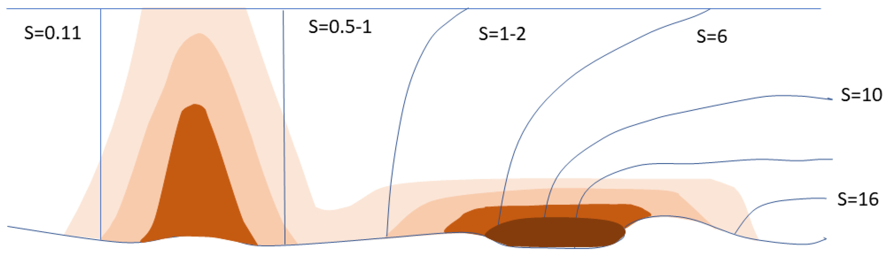
5.2. General Patterns of ETMs

During each of 6 longitudinal transects operated in early wet season in the Cam-Nam Trieu estuary, we observed and measured two kinds of Estuarine Turbidity Maxima: an upper ETM was observed in well mixed waters all over the water column (and may thus be visible on ocean color satellite data), while a lower (or downstream) ETM developed only in the bottom boundary layer (Figure 10). The upper ETM started at salinity around 0.11 psu and ended at salinity lower than 0.5 or 1 psu, while the lower ETM ranges for higher salinity values until around 15 psu. A similar structure was repeated 6 times during the 3-days of field survey. The lower limit of the upper ETM and the upper limit of the lower ETM seemed to depend on the stratification of waters and on corresponding values of salinity which are changing during the tidal cycle. The local increase of D50 observed along each transect at salinity values between 0.11 and 0.2 psu in the upper ETM may indicate that flocculation starts at these low salinity values.
We measured a 8-km course of both ETMs between high tide and low tide (see on the kml file v66 at high tide and v19 at low tide for the upper ETM, v75 at high tide and v23 at low tide for the lower ETM). At some stations, our small flat-bottom boat had to escape the main deep channel for shallower waters because of a cargo’s journey. The consistent travel of ETMs moving upstream at high tide and downstream at low tide supports the idea that the local influence of the water depth was not sufficient to generate extra turbidity maximum areas along several consecutive stations.
Multiple ETMs have been recognized in some estuaries. Roberts and Pierce [72] found two ETMs in the upper Patuxent estuary, one corresponding to the salt front and the other to a downstream constriction in the estuary channel. In the Tay estuary, multiple turbidity maxima were reported by Buller [73] and Dobereiner and McManus [74]. Jay and Musiak [12] reported that 3 simultaneous ETMs were observed in the Columbia River estuary, two landward ones located near the upstream limit of salt intrusion and a more seaward one. A double ETM was also reported in the Gironde estuary [7,75].
In this study, at low tide and during flood tide, the upper ETM was observed at salinities between 0.12 psu and less than 0.3 psu (from 0.10–0.15 until 0.12–0.3 psu), while it was observed between 0.11 or 0.12 and 1 psu at ebb tide or high tide. Its main characteristics were to be well mixed (Φ was about 0.74–2.05 and Ri in the range 0.05–0.23, Table 1). This upper ETM may be attributed to flocculation of chemical origin, due to the present ions even at low salinity (here around 0.11–0.12 psu). Many ETMs have been reported at the freshwater-saltwater interface, such as in the Tamar estuary [76].
The lower ETM in the Cam-Nam Trieu estuary developed in much varying salinity ranges, starting at 0.25, 0.35, 0.4 or 0.5 psu until around 1 psu or more during low tide and flood tide, while it was observed at salinities between 5 and 15 psu at high tide and between 8 and 15 psu during ebb tide. In fact, the lower ETM developed when the stratification became strong enough (Φ was about 1.22–86.99 and Ri varied in the range 0.11–1.53, Table 1).
The formation of an ETM in the lower estuary (at high salinity) was reported in some previous studies. ETMs in Lorient and Vilaine Bays developed at salinities about 18 psu and 25–30 psu, respectively [77]. In the Weser Estuary an ETM was observed at 6 psu [76]. The salinity stratification was a main factor contributor to ETMs in lower estuary part. This has been confirmed and addressed by numerous studies (e.g., [12,78,79,80,81]). Geyer [26] demonstrated its existence right after the water column becomes stratified. As a result, turbulent mixing is substantially suppressed. Since the sediment is kept in suspension by an approximate balance between gravitational sinking and turbulent mixing, a reduction of vertical mixing will then result in suspended sediment being kept near the bottom. In some cases, suppression of turbulence by salinity stratification increases settling and trapping of fine sediment and may be a more effective trapping mechanism than gravitational circulation [26,82].
Conceptual models of the pathways of fine sediment were proposed by Wolanski et al. [83] for the Mekong River estuary in dry and in wet season. They differ from a season to another since the Mekong estuary is much more mixed in low-flow season. During the high-flow season a salt wedge showed fresh water with salinity almost 0 at the surface flowing over waters with salinity >15 psu along a distance of around 10 km. In this configuration, the Mekong ETM near the bottom is rather short between 0 and 15 psu (<2 km) since the transition between these salinity values is done over a very short distance. In low-flow season, salinity of partially well-mixed waters varied from 0 to 20 along around 30 km, the ETM being concentrated in the bottom layer at salinity between 0 and 15 psu. Its length may be 10 times more (~20 km) and the ETM was located further upstream than in the high-flow season. The conceptual model we can derive from the present study for the lower ETM is consistent with the configuration proposed by Wolanski et al. [83].
A configuration with two ETMs, one surface ETM and one bottom ETM at higher salinities was already described in the San Francisco Bay [79] and in the York River estuary [80]. From 48 surveys spanning a 4-year period, Schoellhamer [79] reported that a surface ETM was always located in the salinity range of 0–2 psu in the northern San Francisco Bay and that a bottom ETM was sometimes located in the salinity range 10–25 psu. In the York River Estuary, Lin and Kuo [80] reported that an ETM is usually located near the head of salt intrusion, well mixed, and another ETM is located in the more stratified waters of the lower estuary, with typical SPM concentrations only high in near bottom.
Lastly, we can check that the two parts of the ETM were connected at low tide and extended over a much longer distance than during the high tide: the partial length was 10 and 16 km during transects 2 and 4, respectively, since measurements stopped downstream at salinity around 1 psu, while the full length of the ETM at high tide was 8 km during transect 5. This trend of shorter length at high tide is consistent with the analysis of the Charente ETM by Toublanc et al. [19]. It is likely explained by the salinity distribution. We noticed that the length of the ETMs was strongly dependent on the longitudinal salinity gradients, with much higher gradients at high tide (and thus shorter ETMs) than at low tide.

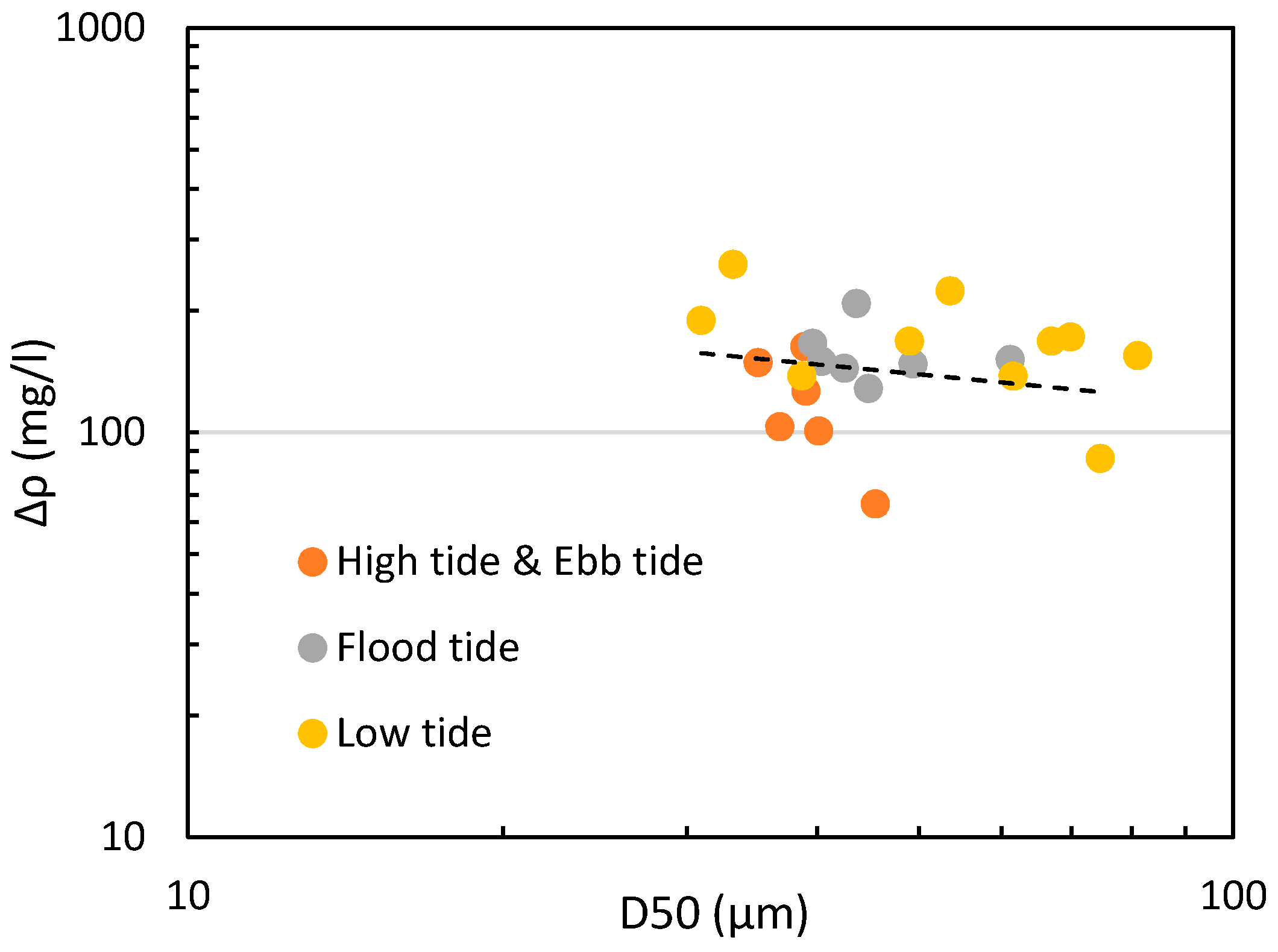
5.3. D50 and Excess of Density of Flocs

The ranges of characteristic parameters in the estuary (D50: 30–90 µm, Δρf: 60–300 kg m−3, ws: 0.07–0.55 mm s−1) are consistent with the values reported in the literature. Guo et al. [84] reported a D50 range (14–95 µm), a range of excess density (60–450 kg m−3) and a settling velocity range (0.04–0.60 mm s−1) in the Yangtze estuary close to our measurements. Manning et al. [85] measured settling velocities between 0.10 and 0.30 mm s−1 for microflocs with diameter 30–80 µm in agreement with our results as well. In the southern North Sea, with SPM concentration in the range 3.6–281 mg L−1 and D50 = 44–88 μm, Fettweis [68] reported excess density varying in the range 117–906 kg m−3.
Ranges for D50 (30–80 µm) and Δρf (60–260 mg L−1) for the 23 sampled waters (Figure 11) are rather short as compared to the variabilities of these parameters compiled by Khelifa and Hill [86] who collected measurements from 26 studies (with 1.5 µm < D < 30000 µm, and 0.01 < Δρf < 1650 mg L−1). Our measurements are consistent with the ones they reported in their Figure 1 and are compatible with a general trend of a decrease in Δρf with increasing D50 [83,84,85,86,87,88]. However, we must note that most of the diameters considered in Khelifa & Hill’study were deduced from image analysis and many values were much higher than the limit imposed by the LISST measurement range. It points that the range of particle diameters which is considered by the LISST is one limit of our study. The range of excess densities obtained in this study (60–300 kg m−3) is highly consistent with reported values of excess density in estuaries in the typical range 50–300 kg m−3 [60].
From our measurements, the median diameter of flocs was the lowest at ebb tide (average D50 = 37.9 μm) and high tide (average D50 = 39.9 μm), intermediate at flood tide (averaged D50 = 45.9 μm), and it was the highest at low tide (averaged D50 = 56.0 μm).
Concerning the fractionation of flocs, we note that the variations of D50 restricted to the fine, medium or coarse size ranges do not strictly follow the variation of the D50 obtained for the whole pool of suspended particles. For example, at high tide, D50 of full range (1.48–212 μm) was the smallest while D50 of coarse flocs (92.6–212 μm) was the highest (Table 1). At low tide, D50 over the whole range was the highest but the average D50 of coarse flocs (92.6–212 μm) was the smallest (Table 1).
We also noticed that the smallest floc sizes were observed at the surface between the upper and lower ETMs. They may result from the settling of flocs in both ETMs. Generally, we also observed in the same area amongst the highest floc sizes near the bed, which may indicate that this transition zone is favorable to deposition.

5.4. Fractal Dimension

Measurements over 23 samples provided values of excess of density for flocs in the range 60–260 kg m−3. Estimates provided by a combination of the Stokes formula and of works by Kranenburg [64] and Maggi [65] which involve the fractal dimension of flocs provided a very good agreement with measurements with df = 2. The adjustment value by value of Δρf to the measured excess of density enabled to derive the fractal dimension for each sample. We obtained df values between 1.93 at high tide and 2.04 at low tide. Smaller df values correspond to lower density flocs, that are therefore more subject to breakup: fragmentation is enhanced and smaller flocs are formed. In contrast, larger df values yield denser flocs, more resistant to breakup. Winterwerp [60] reported that the typical value of df varies from about 1.4 for fragile flocs to about 2.2 for strong estuarine flocs (with a best fit = 2.0 over the whole pool of flocs) as in the Ems and Tamar estuaries. Tambo and Watanabe [87] reported values for mud flocs between 2.0 and 2.25. Fettweis [68] reported that the floc fractal dimension calculated from in situ measurements varied typically from 1.6 to 2.3 and that uncertainties remain on its accuracy. In wet season in the Yangtze Estuary, Guo et al. [84] reported df values varying between 1.5 and 2.1 (around a best fit = 1.8). Based on measurements in the Seine estuary, Verney et al. [89] reported df values between 1.62 and 1.82, with a mean of 1.75. From observations of particle cross-sectional area and mass performed along the south and west coasts of Great Britain, Bowers et al. [90] showed that df varied in the range 1.9–2.7. All these published results comfort us on the range of df values estimated in this study.
The tidal variation of df values tends to indicate that flocs in the Cam-Nam Trieu estuary were the strongest at low tide (with df = 2.04) and the more fragile at high tide (with df = 1.93).

5.5. Settling Velocity of Flocs

The settling velocity of flocs (ws) is the most sensitive parameter to estimate sediment accumulation. ws may be reduced by the hindering of other flocs [16,61,62,91] at high concentration (much more than the maximum concentration measured here). The permeability of highly porous aggregates significantly affects their settling velocity [92,93,94]. In this study, estimates of floc settling velocities during the survey varied between 0.07 and 0.55 mm s−1. They were estimated to vary between 0.12 and 0.40 mm s−1 in the core of the ETMs. Their values were the highest in ETMs at low tide (0.28–0.40 mm s−1, transects 2 and 4), high in ETMs during flood tide (0.15–0.26 mm s−1, transects 1 and 3), low in ETMs at ebb tide (0.15–0.17 mm s−1) and they were the lowest at high tide (0.12–0.14 mm s−1) (Table 1). These results are similar to values reported in the literature. In a tidal creek that drained a salt marsh, Voulgaris and Meyers [45] recorded mean floc sizes of 25–75 μm, SPM concentrations less than 80 mg L−1 and settling velocities between 0.02 and 0.20 mm s−1. In the Pearl River Estuary (China), with SPM concentrations typically less than 100 mg L−1, median floc sizes varied between 10 and 96 μm and settling velocities between 0.01 and 0.20 mm s−1, with values increasing with increasing floc size [95]. In the Seine estuary (with SPM in the range 10–200 mg L−1), Verney et al. [89] estimated the settling velocities of flocs in the range 0.07–0.50 mm s−1. In the Yangtze Estuary (with SPM ranging from 100 to 7000 mg L−1) in the wet season, settling velocities of flocs were estimated between 0.04 and 0.60 mm s−1 [84]. The range of our estimates in the Cam-Nam Trieu estuary (0.07–0.55 mm s−1) is thus consistent with values obtained in other similar environments. In complement, the percentages of fine, medium and coarse aggregates showed to be consistent with this temporal evolution of ws since we measured the highest proportion of coarse particles at low tide, with the highest ws (see transects 2 and 4, Table 1) and the highest proportion of fine aggregates at high tide, with the smallest ws (see transect 5, Table 1).
ws values showed to be highly correlated with SPM (R2 = 0.58, Figure 12a) and D50 (R2 = 0.68, Figure 12b), through power law relationships. The values of SPM and ws were the smallest at high tide and ebb tide (<60 mg L−1 and <0.13 mm s−1), intermediate at flood tide (60–110 mg L−1 and 0.12–0.31 mm s−1), and spread over a larger range at low tide (85–230 mg L−1 and 0.10–0.46 mm s−1) (Figure 2a and Figure 12a). D50 values were lower at high tide and ebb tide (35–45 µm) than at flood tide (40–62 µm), and the range was enlarged at low tide (30–85 µm) (Figure 12). Higher values of D50 at flood tide than at ebb tide was already observed by Lefebvre et al. [38] who also showed that turbulence was a strong forcing on D50. In their study, the Kolmogorov microscale (i.e., the size of the smallest turbulent eddies) was shown to limit the maximum floc size at a given period of the tide cycle.
The correction factor on the settling velocity accounting for the turbulence generated by the flocs themselves (Equation (9)) was calculated for the 23 values of ws derived from measurements (LISST and filtration), so as to estimate its potential influence. Over 23 samples, we obtained Rep = 0.012 in average (between 0.002 and 0.044). In consequence, the correction on ws by Winterwerp’s formula (Equation (9)) provided ws values in average 0.64% lower than the original ws. This correction can thus be neglected in our study.

5.6. On the Origins of ETMs in the Cam-Nam Trieu Estuary

At spring tide in early wet season with intermediate river discharge, the Cam-Nam Trieu estuary exhibits a salt wedge. Its upper part is well mixed until salinity around 1 psu, then its downstream part is stratified. The range of salinity values at which we observed ETMs from less than 1 psu to ~15 psu is consistent with other ETMs described in the literature by [16,84]. Two main origins have been proposed to explain the formation of Turbidity Maximum in estuaries.
The first mechanism involves residual currents associated with gravitational circulation in partially mixed estuaries. In this configuration, the salinity distribution drives a residual flow near the bottom directed landward and a residual surface flow directed seaward. When sediments brought at the surface starts to flocculate, they settle and are moved back landward near the bed towards the estuary head. The gravitational circulation happens when isohalines starts to be inclined, in partially stratified areas. The derived Turbidity Maximum is located near the limit of salt intrusion.
The second mechanism relates to the non-linear interactions between the tide and the channel morphology. Distortion causes flows to be shorter and more energetic during flood tide than during ebb tide [21]. This tidal asymmetry causes a net transport of sediment oriented landward until a null point where the seaward flow has a transport competency similar to that of the flooding tide [96]. The role of salinity gradients is to maintain the turbidity maximum in the estuary [13]. As tidal asymmetry was already shown to infer a net flux of suspended matter landward by tidal pumping [38], this mechanism is present in the Cam-Nam Trieu estuary and may explain the formation of the lower ETM. However, as stratification is also settling and increasing downwards around the lower ETM, the gravitational circulation may also participate to this ETM formation. This latter process is hypothesized to be of second order in the Cam-Nam Trieu estuary since the concentrations of SPM are rather low as compared to many other estuaries where SPM concentration can be higher than 1 g L−1.
In some estuaries, the two processes can be alternatively at the origin of the ETM at different tidal periods. In the Seine River estuary for example, Brenon and Le Hir [13] showed that the gravitational circulation was the cause of ETM in neap tide while the tidal asymmetry explained the existence of the ETM in spring tide. Both processes were also shown to participate coincidently to the ETM formation in a micro-tidal estuary of Australia [97]. Here, we wonder if the two processes may participate to form the lower ETM which evidenced sometimes 2 zones of turbidity maxima in the salt wedge.
A third process may be considered as well in the ETM building in the Cam-Nam Trieu estuary. The lower ETM was observed in the region of high salinity range (between ~1 and 15 psu). Eisma [98] indicated that salt-induced salinity flocculation is complete at 8 psu or less. Additional processes may explain flocculation at higher salinity values, like the influence of Exopolymer Substances. Indeed, their stickiness is the highest between 10 and 15 psu [39] and they were shown to contribute to bio-induced flocculation in this estuary. The formation and location of the lower ETM may thus result from different complementary contributions.
Several hypotheses may be drawn regarding the formation of the upper ETM. It may be formed by the flocculation of fine particles starting at low salinity values (around 0.11 psu), by the sudden increase of available ions. The upper ETM may also correspond to the transport of suspended matter eroded in the lower ETM by the tidal asymmetry, between the density node and the tidal node (as shown by [21], their Figure 13). As suggested by several authors [13,22,99], the tidal asymmetry was certainly essential to support the existence of an ETM while the density gradients likely act on its stability and shape, and against the exit of sediments offshore. This may explain the shape of the full ETM with two distinct part: one over the mixed and slightly salted waters, and another over the partially mixed waters at low salinity (up to 15 psu). Numerical simulations of the sediment transport within this estuary may help us to check which processes are acting and are mainly responsible of the observed turbidity patterns, like other authors did (e.g., [13]). The role of bottom topography (which may enhance salinity stratification and gravitational circulation like in the San Francisco bay, see [79]) may also be investigated using a numerical model.
Open questions still remain on the origin(s) of the ETM in the Cam-Nam Trieu estuary. The analysis of field measurements performed in the same estuary at other seasons will enable to further analysis the seasonal variability of the Turbidity Maximum areas in future papers, and to compare its dynamics with the one of other ETMs like Sottolichio and Castaing [7], Jalon-Rojas et al. [99] and Uncles et al. [100] did, for example.

Supplementary Materials

The following are available online at www.mdpi.com/2073-4441/10/1/68/s1. Figure S1: supplementary.v1.kml.

Acknowledgments

This work was financed by the science and technological cooperation program between the Vietnam Academy of Sciences and Technology (VAST), the Hanoi University of Science of the Vietnam National University (HUS-VNU) and the French Institut de Recherche pour le Développement (IRD), in the frame of the PhD studies of Vu Duy Vinh, and by the project NĐT.01.CHN/15. Vinh belongs to the Institute of Marine Environment and Resources (VAST, Haiphong), he is registered at the doctoral school of the University of Science and Technology of Hanoi (USTH) and this study was developed in the Hanoi International Laboratory of Oceanography (HILO) of USTH.

Author Contributions

V.D.V., D.V.U. and S.O. conceived the study; V.D.V. and S.O. organized the field trip; V.D.V. performed preliminary analysis; V.D.V., D.V.U. and S.O. analyzed the data; V.D.V. and S.O. wrote the paper.

Conflicts of Interest

The authors declare no conflict of interest.

References

  1. Fettweis, M.; Sas, M.; Monbaliu, J. Seasonal, Neap-spring and tidal variation of cohesive sediment concentration in the Scheldt estuary, Belgium. Estuar. Coast. Shelf Sci. 1998, 47, 21–36. [Google Scholar] [CrossRef]
  2. Mitchell, S.B.; Uncles, R.J. Estuarine sediments in macrotidal estuaries: Future research requirements and management challenges. Ocean Coast. Manag. 2013, 79, 97–100. [Google Scholar] [CrossRef]
  3. Kistner, D.A.; Pettigrew, N.R. A variable turbidity maximum in the Kennebec Estuary. Estuaries 2001, 24, 680–687. [Google Scholar] [CrossRef]
  4. Uncles, R.J.; Stephens, J.A.; Smith, R.E. The dependence of estuarine turbidity on tidal intrusion length, tidal range and residence time. Cont. Shelf Res. 2002, 22, 1835–1856. [Google Scholar] [CrossRef]
  5. Kirby, R.; Parker, W.R. Distribution and behavior of fine sediment in the Severn Estuary and Inner Bristol Channel, UK. Can. J. Fish. Aquat. Sci. 1983, 40, 83–95. [Google Scholar] [CrossRef]
  6. Allen, G.P.; Castaing, P. Suspended sediment transport from the Gironde estuary (France) onto the adjacent continental shelf. Mar. Geol. 1973, 14, 47–53. [Google Scholar] [CrossRef]
  7. Sottolichio, A.; Castaing, P. A synthesis on seasonal dynamics of highly concentrated structures in the Gironde estuary. Comptes Rendus l’Acad. Sci. Paris IIa 1999, 329, 895–900. [Google Scholar] [CrossRef]
  8. Jalón-Rojas, I.; Schmidt, S.; Sottolichio, A. Turbidity in the fluvial Gironde Estuary (southwest France) based on 10-year continuous monitoring: Sensitivity to hydrological conditions. Hydrol. Earth Syst. Sci. 2015, 19, 2805–2819. [Google Scholar] [CrossRef]
  9. Olsen, C.R.; Simpson, H.J.; Bopp, R.F.; Williams, S.C.; Peng, T.H.; Deck, B.L. A geochemical analysis of the sediments and sedimentation in the Hudson estuary. J. Sediment. Petrol. 1978, 48, 401–418. [Google Scholar]
  10. Geyer, W.R.; Woodruff, J.D.; Traykovski, P. Sediment transport and trapping in the Hudson River Estuary. Estuaries 2001, 24, 670–679. [Google Scholar] [CrossRef]
  11. Traykovski, P.; Geyer, W.R.; Sommerfield, C. Rapid sediment deposition and fine-scale strata formation in the Hudson estuary. J. Geophys. Res. 2004, 109, F02004. [Google Scholar] [CrossRef]
  12. Jay, D.A.; Musiak, J.D. Particle trapping in estuarine tidal flows. J. Geophys. Res. 1994, 99, 20445–20461. [Google Scholar] [CrossRef]
  13. Brenon, I.; Le Hir, P. Modelling the turbidity maximum in the Seine estuary (France): Identification of formation processes. Estuar. Coast. Shelf Sci. 1999, 49, 525–544. [Google Scholar] [CrossRef]
  14. Sanford, L.P.; Suttles, S.E.; Halka, J.P. Reconsidering the physics of the Chesapeake Bay estuarine turbidity maximum. Estuaries 2001, 24, 655–669. [Google Scholar] [CrossRef]
  15. Sanford, L.P.; Dickhudt, P.J.; Rubiano-Gomez, L.; Yates, M.; Suttles, S.E.; Friedrichs, C.T.; Fugate, D.D.; Romine, H. Variability of suspended particle concentrations, sizes, and settling velocities in the Chesapeake Bay turbidity maximum. In Flocculation in Natural and Engineered Environmental Systems; Droppo, I.G., Leppard, G.G., Liss, S.N., Milligan, T.G., Eds.; CRC Press: Boca Raton, FL, USA, 2005; pp. 211–236. [Google Scholar]
  16. Uncles, R.J.; Stephens, J.A.; Harris, C. Runoff and tidal influences on the estuarine turbidity maximum of a highly turbid system: The upper Humber and Ouse Estuary, UK. Mar. Geol. 2006, 235, 213–228. [Google Scholar] [CrossRef]
  17. Postma, H. Sediment transport and sedimentation in the estuarine environment. In Estuaries; Lauff, G.H., Ed.; American Association Advanced Scientific Publication: Washington, DC, USA, 1967; pp. 158–179. [Google Scholar]
  18. Bowden, K.F. Turbulence and mixing in estuaries. In The Estuary as a Filter; Kennedy, V.S., Ed.; Academic Press: Orlando, FL, USA, 1984; pp. 15–26. [Google Scholar]
  19. Toublanc, F.; Brenon, I.; Coulombier, T. Formation and structure of the turbidity maximum in the macrotidal Charente estuary (France): Influence of fluvial and tidal forcing. Estuar. Coast. Shelf Sci. 2016, 169, 1–14. [Google Scholar] [CrossRef]
  20. Schubel, J.R. Turbidity maximum of the northern Chesapeake Bay. Science 1968, 161, 1013–1015. [Google Scholar] [CrossRef] [PubMed]
  21. Allen, G.P.; Salomon, J.C.; Bassoullet, P.; du Penhoat, Y.; de Grandpré, C. Effects of tides on mixing and suspended sediment transport in macrotidal estuaries. Sediment. Geol. 1980, 26, 69–90. [Google Scholar] [CrossRef]
  22. Sottolichio, A.; Le Hir, P.; Castaing, P. Modeling mechanisms for the stability of the turbidity maximum in the Gironde estuary, France. Proc. Mar. Sci. 2000, 3, 373–386. [Google Scholar]
  23. Coleman, J.M.; Wright, L.D. Sedimentation in an arid macrotidal alluvial river system: Ord River, Western Australia. J. Geol. 1978, 86, 621–642. [Google Scholar] [CrossRef]
  24. Uncles, R.J.; Stephens, J.A. Nature of the turbidity maximum in the Tamar Estuary, UK. Estuar. Coast. Shelf Sci. 1993, 36, 413–431. [Google Scholar] [CrossRef]
  25. Komar, P.D.; Taghon, G.L. Analyses of the settling velocities of fecal pellets from the subtidal polychaete Amphicteis scaphobranchiata. J. Mar. Res. 1985, 43, 605–614. [Google Scholar] [CrossRef]
  26. Geyer, W.R. The importance of suppression of turbulence by stratification on the estuarine turbidity maximum. Estuaries 1993, 16, 113–125. [Google Scholar] [CrossRef]
  27. Geyer, W.R.; Signell, R.; Kineke, G. Lateral trapping of sediment in a partially mixed estuaries. In Physics of Estuaries and Coastal Seas: Proceedings of the 8th International Biennial Conference on Physics of Estuaries and Coastal Seas, Hague, The Netherlands, 9–12 September 1996; Dronkers, J., Scheffers, M., Eds.; A.A. Balkema: Rotterdam, The Netherlands, 1998; pp. 115–124. [Google Scholar]
  28. Hill, P.S.; McCave, L.N. Suspended Particle Transport in Benthic Boundary Layers. In The Bemic Boundary Layer; Boudreau, B.P., Bo Barker, J., Eds.; Oxford University Press: New York, NY, USA, 2001; pp. 78–103. [Google Scholar]
  29. Hill, P.S.; Voulgaris, G.; Trowbridge, J.H. Controls on floc size in a continental shelf bottom boundary layer. J. Geophys. Res. Oceans 2001, 106, 9543–9549. [Google Scholar] [CrossRef]
  30. Haiphong statistics office. Haiphong Statistics Yearbook 2016; Statistical Publishing house: Hai Phong, Vietnam, 2017.
  31. Vietnam maritime administration (Vinamarine). Approved planning for dredging in Hai Phong port. Available online: http://www.vinamarine.gov.vn (accessed on 29 July 2017).
  32. Vuong, B.V.; Liu, Z.F.; Thanh, T.D.; Khang, N.D. Initial results of study in sedimentation rate and geochronology of modern sediments in the Bach Dang estuary by the methods of 210Pb and 137Cs radio tracer. In Proceedings of the Second National Scientific Conference on Marine Geology, Ha Noi-Ha Long, Vietnam, 10–11 October 2013; pp. 306–315. [Google Scholar]
  33. Thanh, T.D.; Can, N.; Nga, D.D.; Huy, D.V. Coastal development and sea level change during Holocene in Haiphong area. J. Mar. Sci. Technol. 2004, 3, 25–42. [Google Scholar]
  34. Cu, N.V.; Huong, N.T.T.; Cham, D.D. Causes and Proposal Solution for Deposition in Navigation Channel to Hai Phong Ports. Final Report of the MOST Project; The Institute of Geology: Hanoi City, Vietnam, 1997. (In Vietnamese) [Google Scholar]
  35. Cu, N.V.; Cham, D.D. Research on Hydrodynamics, Sediment Transport, Deposition in Lach Huyen, South Do Son (Hai Phong) by Influenced of the Deep-Port and Propose Solution. Final Report of the KC.08.10/06-10 Project; The Institute of Geology: Hanoi City, Vietnam, 2010. (In Vietnamese) [Google Scholar]
  36. Vinh, V.D.; Thanh, T.D. Application of numerical model to study on maximum turbidity zones in Bach Dang estuary. J. Mar. Sci. Technol. 2012, 3, 1–12. [Google Scholar]
  37. Vinh, V.D.; Uu, D.V. The influence of wind and oceanographic factors on characteristics of suspended sediment transport in Bach Dang estuary. J. Mar. Sci. Technol. 2013, 3, 216–226. [Google Scholar] [CrossRef]
  38. Lefebvre, J.P.; Ouillon, S.; Vinh, V.D.; Arfi, R.; Panche, J.Y.; Mari, X.; Van Thuoc, C.; Torréton, J.P. Seasonal variability of cohesive sediment aggregation in the Bach Dang-Cam Estuary, Haiphong (Vietnam). Geo-Mar. Lett. 2012, 32, 103–121. [Google Scholar] [CrossRef]
  39. Mari, X.; Torréton, J.P.; Chu, V.T.; Lefebvre, J.P.; Ouillon, S. Seasonal aggregation dynamics along a salinity gradient in the Bach Dang estuary, North Vietnam. Estuar. Coast. Shelf Sci. 2012, 96, 151–158. [Google Scholar] [CrossRef]
  40. Vinh, V.D.; Ouillon, S.; Thanh, T.D.; Chu, L.V. Impact of the Hoa Binh dam (Vietnam) on water and sediment budgets in the Red River basin and delta. Hydrol. Earth Syst. Sci. 2014, 18, 3987–4005. [Google Scholar] [CrossRef]
  41. Minh, N.N.; Marchesiello, P.; Lyard, F.; Ouillon, S.; Cambon, G.; Allain, D.; Van Uu, D. Tidal characteristics of the Gulf of Tonkin. Cont. Shelf Res. 2014, 91, 37–56. [Google Scholar] [CrossRef]
  42. Traykovski, P.; Latter, R.; Irish, J.D. A laboratory evaluation of the LISST instrument using natural sediments. Mar. Geol. 1999, 159, 355–367. [Google Scholar] [CrossRef]
  43. Agrawal, Y.C.; Pottsmith, H.C. Instruments for particle size and settling velocity observations in sediment transport. Mar. Geol. 2000, 168, 89–114. [Google Scholar] [CrossRef]
  44. Mikkelsen, O.A.; Pejrup, M. In situ particle size spectra and density of particle aggregates in a dredging plume. Mar. Geol. 2000, 170, 443–459. [Google Scholar] [CrossRef]
  45. Voulgaris, G.; Meyers, S.T. Temporal variability of hydrodynamics, sediment concentration and sediment settling velocity in a tidal creek. Cont. Shelf Res. 2004, 24, 1659–1683. [Google Scholar] [CrossRef]
  46. Mikkelsen, O.A.; Hill, P.S.; Milligan, T.G.; Chant, R.J. In situ particle size distributions and volume concentrations from a LISST-100 laser particle sizer and a digital floc camera. Cont. Shelf Res. 2005, 25, 1959–1978. [Google Scholar] [CrossRef]
  47. Jouon, A.; Ouillon, S.; Douillet, P.; Lefebvre, J.-P.; Fernandez, J.-M.; Mari, X.; Froidefond, J.-M. Spatio-temporal variability in suspended particulate matter concentration and the role of aggregation on size distribution in a coral reef lagoon. Mar. Geol. 2008, 256, 36–48. [Google Scholar] [CrossRef]
  48. Andrews, S.; Nover, D.; Schladow, S. Using laser diffraction data to obtain accurate particle size distributions: The role of particle composition. Limnol. Oceanogr. Methods 2010, 8, 507–526. [Google Scholar] [CrossRef]
  49. Graham, G.W.; Davies, E.J.; Nimmo-Smith, W.A.M.; Bowers, D.G.; Braithwaite, K.M. Interpreting LISST-100X measurements of particles with complex shape using digital in-line holography. J. Geophys. Res. 2012, 117, C05034. [Google Scholar] [CrossRef]
  50. Fettweis, M.; Baeye, M. Seasonal variation in concentration, size and settling velocity of muddy marine flocs in the benthic boundary layer. J. Geophys. Res. Oceans 2015, 120, 5648–5667. [Google Scholar] [CrossRef]
  51. Many, G.; Bourrin, F.; Durrieu de Madron, X.; Pairaud, I.; Gangloff, A.; Doxaran, D.; Ody, A.; Verney, R.; Menniti, C.; Le Berre, D.; et al. Particle assemblage characterization in the Rhone river ROFI. J. Mar. Syst. 2016, 157, 39–51. [Google Scholar] [CrossRef]
  52. Pinet, S.; Martinez, J.M.; Ouillon, S.; Lartiges, B.; Villar, R.E. Variability of apparent and inherent optical properties of sediment-laden waters in large river basins—Lessons from in situ measurements and bio-optical modeling. Opt. Express 2017, 25, A283–A310. [Google Scholar] [CrossRef] [PubMed]
  53. Bader, H. The hyperbolic distribution of particle sizes. J. Geophys. Res. 1970, 75, 2822–2830. [Google Scholar] [CrossRef]
  54. Jackson, G.; Maffione, D.; Costello, A.; Alldredge, B.; Logan, B.; Dam, H. Particle size spectra between 1 μm and 1 cm at Monterey Bay determined using multiple instruments. Deep Sea Res. Part I Oceanogr. Res. Pap. 1997, 44, 1739–1767. [Google Scholar] [CrossRef]
  55. Boss, E.; Twardowski, M.S.; Herring, S. Shape of the particulate beam attenuation spectrum and its inversion to obtain the shape of the particulate size distribution. Appl. Opt. 2001, 40, 4885–4893. [Google Scholar] [CrossRef] [PubMed]
  56. Wozniak, S.B.; Stramski, D. Modeling the optical properties of mineral particles suspended in seawater and their influence on ocean reflectance and chlorophyll estimation from remote sensing algorithms. Appl. Opt. 2004, 43, 3489–3503. [Google Scholar] [CrossRef] [PubMed]
  57. Loisel, H.; Nicolas, J.M.; Sciandra, A.; Stramski, D.; Poteau, A. Spectral dependency of optical backscattering by marine particles from satellite remote sensing of the global ocean. J. Geophys. Res. 2006, 111, C09024. [Google Scholar] [CrossRef]
  58. Jonasz, M. Particle size distribution in the Baltic. Tellus 1983, 35B, 346–358. [Google Scholar] [CrossRef]
  59. Lee, B.J.; Fettweis, M.; Toorman, E.; Molz, F. Multimodality of a particle size distribution of cohesive suspended particulate matters in a coastal zone. J. Geophys. Res. 2012, 117, C03014. [Google Scholar] [CrossRef]
  60. Winterwerp, J.C. A simple model for turbulence induced flocculation of cohesive sediment. J. Hydraul. Res. 1998, 36, 309–326. [Google Scholar] [CrossRef]
  61. Winterwerp, J.C. Stratification effects by cohesive and noncohesive sediment. J. Geophys. Res. 2001, 106, 22559–22574. [Google Scholar] [CrossRef]
  62. Winterwerp, J.C. A heuristic formula for turbulence-induced flocculation of cohesive sediment. Estuar. Coast. Shelf Sci. 2006, 68, 195–207. [Google Scholar] [CrossRef]
  63. Stokes, G.G. On the Effect of the Internal Friction of Fluids on the Motion of Pendulums. In Transaction Cambridge Philosophical Society; Printed at the Pitt Press: Cambridge, UK, 1851; Volume IX, pp. 8–106, Reprinted In Mathematical and Physical Papers, 2nd ed.; Johnson Reprint Corp: New York, NY, USA, 1966; Volume 3. [Google Scholar]
  64. Kranenburg, C. The fractal structure of cohesive sediment aggregates. Estuar. Coast. Shelf Sci. 1994, 39, 451–460. [Google Scholar] [CrossRef]
  65. Maggi, F. Biological flocculation of suspended particles in nutrient-rich aqueous ecosystems. J. Hydrol. 2009, 376, 116–125. [Google Scholar] [CrossRef]
  66. Maerz, J.; Hofmeister, R.; van der Lee, E.M.; Gräwe, U.; Riethmüller, R.; Wirtz, K.W. Maximum sinking velocities of suspended particulate matter in a coastal transition zone. Biogeosciences 2016, 13, 4863–4876. [Google Scholar] [CrossRef]
  67. Van der Lee, E.M.; Bowers, D.; Kyte, E. Remote sensing of temporal and spatial patterns of suspended particle size in the Irish Sea in relation to the Kolmogorov microscale. Cont. Shelf Res. 2009, 29, 1213–1225. [Google Scholar] [CrossRef]
  68. Fettweis, M. Uncertainty of excess density and settling velocity of mud flocs derived from in situ measurements. Estuar. Coast. Shelf Sci. 2008, 78, 426–436. [Google Scholar] [CrossRef]
  69. Ouillon, S.; Douillet, P.; Petrenko, A.; Neveux, J.; Dupouy, C.; Froidefond, J.M.; Andréfouët, S.; Muñoz-Caravaca, A. Optical algorithms at satellite wavelengths for Total Suspended Matter in tropical coastal waters. Sensors 2008, 8, 4165–4185. [Google Scholar] [CrossRef] [PubMed]
  70. Miles, J. Richardson’s criterion for the stability of stratified shear flow. Phys. Fluids 1986, 29, 3470. [Google Scholar] [CrossRef]
  71. Simpson, J.H.; Allen, C.M.; Morris, N.C.G. Fronts on the continental shelf. J. Geophys. Res. 1978, 83, 4607–4614. [Google Scholar] [CrossRef]
  72. Roberts, W.P.; Pierce, J.W. Deposition in upper Patuxent estuary, Maryland, 1968–1969. Estuar. Coast. Mar. Sci. 1976, 4, 267–280. [Google Scholar] [CrossRef]
  73. Buller, A.T. Sediments of the Tay Estuary. II. Formation of Ephemeral Zones of High Suspended Sediment Concentrations. Proc. R. Soc. Edinb. Sect. B Nat. Environ. 1975, 75, 65–89. [Google Scholar] [CrossRef]
  74. Dobereiner, C.; McManus, J. Turbidity Maximum Migration and Harbor Siltation in the Tay Estuary. Can. J. Fish. Aquat. Sci. 1983, 40, s117–s141. [Google Scholar] [CrossRef]
  75. Doxaran, D.; Froidefond, J.M.; Castaing, P.; Babin, M. Dynamics of the turbidity maximum zone in a macrotidal estuary (the Gironde, France): Observations from field and MODIS satellite data. Estuar. Coast. Shelf Sci. 2009, 81, 321–332. [Google Scholar] [CrossRef]
  76. Grabemann, I.; Uncles, R.J.; Krause, G.; Stephens, J.A. Behaviour of Turbidity Maxima in the Tamar (U.K.) and Weser (F.R.G.) Estuaries. Estuar. Coast. Shelf Sci. 1997, 45, 235–246. [Google Scholar] [CrossRef]
  77. Le Bris, H.; Glémarec, M. Marine and brackish ecosystems of south Brittany (Lorient and Vilaine Bays) with particular reference to the effect of the turbidity maxima. Estuar. Coast. Shelf Sci. 1996, 42, 737–753. [Google Scholar] [CrossRef]
  78. Simpson, J.H.; Brown, J.; Matthews, J.; Allen, G. Tidal straining, density currents, and stirring in the control of estuarine stratification. Estuaries 1990, 13, 125–132. [Google Scholar] [CrossRef]
  79. Schoellhamer, D.H. Influence of salinity, bottom topography, and tides on locations of estuarine turbidity maxima in northern San Francisco Bay. In Proceedings in Marine Science; McAnally, W.H., Mehta, A.J., Eds.; Elsevier Science: Amsterdam, The Netherlands, 2000; Volume 3, pp. 343–357. [Google Scholar]
  80. Lin, J.; Kuo, A.Y. Secondary turbidity maximum in a micro-tidal partially mixed estuary. Estuaries 2001, 24, 707–720. [Google Scholar] [CrossRef]
  81. Lin, J.; Kuo, A.Y. A model study of turbidity maxima in the York River Estuary, Virginia. Estuaries 2003, 26, 1269–1280. [Google Scholar] [CrossRef]
  82. Hamblin, P.F. Observations and model of sediment transport near the turbidity maximum of the upper Saint Lawrence Estuary. J. Geophys. Res. 1989, 94, 14419–14428. [Google Scholar] [CrossRef]
  83. Wolanski, E.; Huan, N.N.; Dao, L.T.; Nhan, N.H.; Thuy, N.N. Fine-sediment Dynamics in the Mekong River Estuary, Vietnam. Estuar. Coast. Shelf Sci. 1996, 43, 565–582. [Google Scholar] [CrossRef]
  84. Guo, C.; He, Q.; Guo, L.; Winterwerp, J.C. A study of in-situ sediment flocculation in the turbidity maxima of the Yangtze Estuary. Estuar. Coast. Shelf Sci. 2017, 191, 1–9. [Google Scholar] [CrossRef]
  85. Manning, A.J.; Langston, W.J.; Jonas, P.J.C. A review of sediment dynamics in the Severn estuary: Influence of flocculation. Mar. Poll. Bull. 2010, 61, 37–51. [Google Scholar] [CrossRef] [PubMed]
  86. Khelifa, A.; Hill, P.S. Models for effective density and settling velocity of flocs. J. Hydraul. Res. 2006, 44, 390–401. [Google Scholar] [CrossRef]
  87. Tambo, N.; Watanabe, Y. Physical characteristics of flocs. I. The floc density function and aluminium floc. Water Res. 1979, 13, 409–419. [Google Scholar] [CrossRef]
  88. Dyer, K.R.; Manning, A.J. Observation of the size, settling velocity, and effective density of flocs, and their fractal dimension. J. Sea Res. 1999, 41, 87–95. [Google Scholar] [CrossRef]
  89. Verney, R.; Lafite, R.; Brun Cottan, J.C. Flocculation potential of natural estuarine particles: The importance of environmental factors and of the spatial and seasonal variability of suspended particulate matter. Estuar. Coast. 2009, 32, 678–693. [Google Scholar] [CrossRef]
  90. Bowers, D.G.; McKee, D.; Jago, C.F.; Nimmo-Smith, W.A.M. The area-to-mass ratio and fractal dimension of marine flocs. Estuar. Coast. Shelf Sci. 2017, 189, 224–234. [Google Scholar] [CrossRef]
  91. Winterwerp, J.C. On the Dynamics of High Concentrated Mud Suspensions. Ph.D. Thesis, Delft University of Technology, Delft, The Netherlands, October 1999; 171p. [Google Scholar]
  92. Kranck, K. The role of flocculation in the filtering of particulate matter in estuaries. In The Estuary as a Filter; Kennedy, V., Ed.; Academic Press: Orlando, FL, USA, 1984; pp. 159–175. [Google Scholar]
  93. Mehta, A.J. On estuarine cohesive sediment suspension behaviour. J. Geophys. Res. 1989, 94, 14303–14314. [Google Scholar] [CrossRef]
  94. Johnson, C.P.; Li, X.; Logan, B.E. Settling velocities of fractal aggregates. Environ. Sci. Technol. 1996, 30, 1911–1918. [Google Scholar] [CrossRef]
  95. Xia, X.M.; Li, Y.; Yang, H.; Wu, C.Y.; Sing, T.H.; Pong, H.K. Observations on the size and settling velocity distributions of suspended sediment in the Pearl River Estuary, China. Cont. Shelf Res. 2004, 24, 1809–1826. [Google Scholar] [CrossRef]
  96. Dyer, K.R. Coastal and Estuarine Sediment Dynamics; John Wiley & Sons: Chichester, UK, 1986; 342p. [Google Scholar]
  97. Hugues, M.G.; Harris, P.T.; Hubble, C.T. Dynamics of the turbidity maximum zone in a micro-tidal estuary: Hawkesbury River, Australia. Sedimentology 1998, 45, 397–410. [Google Scholar] [CrossRef]
  98. Eisma, D. Suspended Matter in the Aquatic Environment; Springer: Berlin, Germany, 1993. [Google Scholar]
  99. Jalon-Rojas, I.; Schmidt, S.; Sottolichio, A.; Bertier, C. Tracking the turbidity maximum zone in the Loire estuary (France) based on a long-term, high-resolution and high-frequency monitoring network. Cont. Shelf Res. 2016, 117, 1–11. [Google Scholar] [CrossRef]
  100. Uncles, R.J.; Barton, M.L.; Stephens, J.A. Seasonal Variability of fine-sediment concentrations in the Turbidity Maximum region of the Tamar estuary. Estuar. Coast. Shelf Sci. 1994, 38, 19–39. [Google Scholar] [CrossRef]
Figure 1. The Cam-Nam Trieu estuary (a) general location–transects were mostly performed between stations A and B, C is the hydrological station, D is the tide gauge at Hon Dau; (b) example of survey (stations of Transect 4) along the A-B transect.
Water 10 00068 g001aWater 10 00068 g001b
Figure 2.ρf and ws in the Cam-Nam-Trieu estuary in May 2015: (a) variation of ∆ρf and ws (based on the measured ∆ρf) during the tide cycle; (b) ratio of ws (based on the fractal distribution of flocs, Equation (8)) and ws based on the measured ∆ρf (Equations (2) and (5)) as compared to ws based on the measured ∆ρf.
Water 10 00068 g002aWater 10 00068 g002b
Figure 3. 2D distributions of parameters along Transect 1 during flood tide (water elevation = 1.3–2.5 m, 10 May 2015). (a) Turbidity (FTU); (b) Salinity (psu); (c) D50 in the whole grain size range (1.48–212 μm); (d) Settling velocity of flocs (mm s−1); (e) PSD slope.
Water 10 00068 g003
Figure 4. Examples of particle size spectra at the core of ETM in the transect 6, during ebb tide. Upper ETM-v104: (a) particle volume concentration per µm; (b) particle number distribution (used to estimate the Junge parameter J). Lower ETM-v95: (c) particle volume concentration; (d) particle number distribution. The tail of PSD slopes is visible for particles <3.38 μm. Best-fit power law relationships given in these figures were calculated for classes #2 to #31.
Water 10 00068 g004
Figure 5. 2D distributions of parameters along Transect 2 during low tide (water elevation = 0.6–0.7 m, 11 May 2015). (a) Turbidity (FTU); (b) Salinity (psu); (c) D50 in the whole grain size range (1.48–212 μm); (d) Settling velocity of flocs (mm s−1); (e) PSD slope.
Water 10 00068 g005
Figure 6. 2D distributions of parameters along Transect 3 during flood tide (water elevation = 1.3–2.4 m, 11 May 2015). (a) Turbidity (FTU); (b) Salinity (psu); (c) D50 in the whole grain size range (1.48–212 μm); (d) Settling velocity of flocs (mm s−1); (e) PSD slope.
Water 10 00068 g006
Figure 7. 2D distributions of parameters along Transect 4 during low tide (water elevation = 0.7–0.8 m, 12 May 2015). (a) Turbidity (FTU); (b) Salinity (psu); (c) D50 in the whole grain size range (1.48–212 μm); (d) Settling velocity of flocs (mm s−1); (e) PSD slope.
Water 10 00068 g007
Figure 8. 2D distributions of parameters along Transect 5 during high tide (water elevation = 2.5–2.7 m, 12 May 2015). (a) Turbidity (FTU); (b) Salinity (psu); (c) D50 in the whole grain size range (1.48–212 μm); (d) Settling velocity of flocs (mm s−1); (e) PSD slope.
Water 10 00068 g008
Figure 9. 2D distributions of parameters along Transect 6 during ebb tide (water elevation = 1.5–2.4 m, 13 May 2015). (a) Turbidity (FTU); (b) Salinity (psu); (c) D50 in the whole grain size range (1.48–212 μm); (d) Settling velocity of flocs (mm s−1); (e) PSD slope.
Water 10 00068 g009
Figure 10. General pattern of ETMs in the Cam-Nam Trieu estuary in early wet season 2015. Isohaline lines are given in blue (with salinity in psu) and turbidity patterns are showed in brown with darker color for higher turbidity values.
Water 10 00068 g010
Figure 11. Covariation of measured values of D50 and excess of density Δρf for 23 samples, May 2015.
Water 10 00068 g011
Figure 12. Sensitivity of ws to SPM concentration (a) and to D50 (b) on 23 samples, May 2015.
Water 10 00068 g012
Table 1. Mean values of some parameters in the longitudinal transects.
Tidal Phase/TransectUpstream in Cam River (Station C)Mean Salinity (psu)Grain Size Group
Fine Flocs (1.48–17.7 μm)Medium Flocs (17.77–92.6 μm)Coarse Flocs (92.6–212 μm)Full Range (1.48–212 μm)
Q (m3 s−1)SPM (mg L−1)D50 (μm)Volume (%)ws (mm s−1)JD50 (μm)Volume (%) ws (mm s−1)JD50 (μm)Volume (%)ws (mm s−1)JD50 (μm)ws (mm s−1)J
Flood tide/transect 1−235.256.30.188.3022.280.0313.2344.7735.160.1743.48131.8441.560.5223.8464.480.2533.37
Low tide/transect 21252.5*0.308.3718.910.0353.2347.8837.530.2063.35130.9643.560.5803.9672.240.3163.36
Flood tide/transect 3137.0113.00.927.9428.300.0263.4042.9335.990.1433.7129.9935.710.4364.0451.430.1723.55
Low tide/transect 41210.0*0.228.3920.220.0373.2047.0037.630.2213.42131.6742.160.6424.0069.370.3333.37
High tide/transect 5−463.8*6.768.2527.860.0203.1141.0335.720.0943.82134.2936.430.2963.5951.070.1163.37
Ebb tide/transect 61096.0107.04.158.5825.790.0243.0842.3738.770.1133.73131.3835.440.3453.8752.830.1413.38
* Only values at ebb and flood were provided by the NHMS at station C.
Table 2. Length and ranges of turbidity and salinity of the ETM parts, and characteristic parameters at selected stations in the Cam-Nam Trieu estuary, May 2015: Richardson number, Simpson parameter, depth-averaged D50, ws and J values (J was calculated over the whole size range 1.48–212 µm).
TransectUpper ETMLower ETM
L (km)Turb. (NTU)S (psu)StationRiΦD50 (µm)wsJL (km)Turb. (NTU)S (psu)StationRiΦD50 (µm)wsJ
FullFineMediumCoarseFullFineMediumCoarse
1 Flood tide3100–2500.13–0.35v60.130.9871.738.2946.52132.730.283.34(1)125–3001–4v1-57.1262.868.1344.99131.270.263.51
2 Low tide4200–3000.15–0.25v210.050.9765.508.5146.42130.950.283.44(5)700–10000.4–1.2v240.111.2256.87.8247.75136.100.253.50
3 Flood tide4120–4500.1–0.15v370.051.8645.827.9943.12127.820.153.606150–9000.3–10v300.2886.9950.878.3742.10130.330.173.55
4 Low tide4120–2500.1–0.12v460.060.7478.588.5548.81133.100.383.279150–2800.14–1.0v620.193.0664.207.9546.93133.530.313.55
5 High tide1100–1200.2–0.8v720.202.0554.207.7042.97133.740.123.551–1.5100–2506–12v821.5380.9362.078.4641.53136.810.143.25
6 Ebb tide4120–2000.15–0.8v1040.231.6357.108.5044.57131.520.163.402100–2004–10v951.1666.6455.658.7641.45135.380.153.36

