Abstract
Polder watercourses within agricultural areas are affected by high chemical oxygen demand (COD) and biological oxygen demand (BOD5) concentrations, due to intensive farming activities and runoff. Practical cases have shown that constructed wetlands (CWs) are eco-friendly and cost-effective treatment systems which can reduce high levels of organic and nutrient pollution from agricultural discharges. However, accumulated recalcitrant organic matter, originated by in-situ sources or elements of CWs (i.e., plants or microbial detritus), limits the fulfilment of current COD discharge threshold. Thus, to evaluate its relevance regarding rivers ecosystem health preservation, we analysed the response of bio-indicators, the Multimetric Macroinvertebrate Index Flanders (MMIF) and the occurrence of organic pollution sensitive taxa towards organic pollutants. For this purpose, statistical models were developed based on collected data in polder watercourses and CWs located in Flanders (Belgium). Results showed that, given the correlation between COD and BOD5, both parameters can be used to indicate the ecological and water quality conditions. However, the variability of the MMIF and the occurrence of sensitive species are explained better by BOD5, which captures a major part of their common effect. Whereas, recalcitrant COD and the interaction among other physico-chemical variables indicate a minor variability on the bio-indicators. Based on these outcomes we suggest a critical re-evaluation of current COD thresholds and moreover, consider other emerging technologies determining organic pollution levels, since this could support the feasibility of the implementation of CWs to tackle agricultural pollution.
1. Introduction
Throughout the years, the environmental limits imposed by the European Water Framework Directive (EU WFD) (2000/60/EC) have become stricter. The aim is to protect and prevent a further decline of the ecological and chemical water status of European fresh and brackish watercourses. By 2027, all surface watercourses should reach ‘good ecological and chemical conditions’ [1,2]. In Flanders (Belgium) these goals are far from being met; since a great majority of surface watercourses, especially polder watercourses have been affected by intensive agricultural practices, causing erosion and excessive spread of manure as fertilizer [3].
Wastewater and agricultural run-off discharged into streams or lakes with high content of organic pollution affect animal and plant life. On the one hand, organic matter (OM) concentrations in watercourses are analysed and measured by the biological oxygen demand (BOD5) and the chemical oxygen demand (COD). Their quantification is based on the amount of oxygen needed to degrade OM. The BOD5 test measures the amount of oxygen consumed by aerobic biological organisms to decompose the organic matter; in contrast to the COD test, which determines the total amount of oxygen needed to oxidize inorganic and organic contaminants, dissolved or suspended in surface water. On the other hand, the ecological status of aquatic ecosystems is determined by metrics and indices. These are derived by several factors such as richness, evenness, diversity, sensitivity and dominance of bio-indicators, such as macroinvertebrates which are linked to the morphology, hydrology, nutrients, salinity, dissolved oxygen (DO), BOD5 and COD contents in watercourses [4,5]. In Flanders, the surface water quality and the ecological conditions of these systems are evaluated by the Flemish Environment Agency (VMM) on monthly and yearly basis, as this agency oversees the fulfilment of environmental policies in Flanders.
Throughout the EU member states, one of the techniques used for the treatment of agricultural and industrial wastes, or run-off are constructed wetlands (CWs), which have been tested and catalogued as a cost-effective an eco-friendly water treatment technique [3,6,7,8,9,10]. Since agricultural wastes and their proper management are the central target for the EU WFD, strict discharge limits have been imposed to the effluents coming from CWs treating animal manure. Moreover, in Flanders it is required that CWs’ yearly average removal efficiencies achieve at least 75% of COD, 90% of BOD5 and 70% of suspended solids (SS) [11]. However, due to recalcitrant organic matter originated by external inputs (organic wastewater) and in-situ sources (microbial and plant detritus), reported and practical cases have shown that COD levels at CWs effluents are above the current thresholds. Considering the numerous advantages of CWs to cope with organic pollution following an environmentally-sensitive approach, Van den Broeck et al. [12] highlighted the need to set more consistent and easily applicable environmental limits for small wetlands and watercourses. So far, most of the emission limit values (ELVs) and environmental quality standard (EQS) set by the EU WFD have been defined on basis of large waterbodies and CWs larger than 50 ha.
Looking at the broader context, congruence and obligations between EU member states have restricted a comprehensible and appropriate implementation of the European water policies. Some of the main limiting factors are the complexity of understanding the ecosystem functioning, knowledge transfer between political institutions and researchers, as well as the lack of or inadequacy of data collection [13]. For example, Table A1 shows how COD and BOD5 discharge standard limits vary between distinct types of industrial wastewater versus CWs effluents.
To encourage the application of CWs to treat agricultural wastewater, the present study investigates the ecological relevance of the current COD discharge standard limit imposed to CWs treating animal manure. For this purpose, multivariate regression models and linear probability models were developed for case specific scenarios, to estimate the possible effects of different physico-chemical concentrations on the ecological status of polder watercourses. For this purpose, the Multimetric Macroinvertebrate Index Flanders (MMIF) was considered as a response variable, as this was adapted to measure the ecological water quality of watercourses according to the river type they belong and to cope with the implementation of the EU WFD [4]. Likewise, the presence of pollution sensitive taxa in polder watercourses was evaluated to have a better insight respect to organic pollution. A study group of macroinvertebrates was selected based on their tolerance score in relation to the MMIF and their saprobic index as presented by Tachet et al. [14]. In this manner, taxa used as key elements to shape the ecosystem stability were inspected for sensitivity towards organic stressors. It is important to note that in this study, other physico-chemical variables were considered for data exploration and statistical regression analysis to indicate the relative importance and interactions of other steering factors determining the health of the receiving river ecosystem.
By assessing the response of the MMIF and sensitive taxa to organic pollution, assumed to be represented by COD, BOD5 and DO concentrations, it is expected to indicate if CWs’ effluent treating animal manure would affect the health and stability of the receiving polder watercourses. In case of negligible effects, the implementation of CWs in vulnerable agricultural lands could be supported. In addition, through this study, flaws and opportunities to delineate standard limits are intended to be highlighted.
The present manuscript is outlined as follows: the materials and methods section indicates the inspection and distribution of physico-chemical and biological data in relation to environmental and discharge standard limits. Then, it describes how data was processed to develop the subsequent multivariate and linear probability models. In Section 3, the results of data analysis and developed models are shown. Finally, the discussion and conclusion sections incorporate an evaluation of the study outcomes regarding the EU WFD and current environmental policies and COD, BOD5 standard limits applied in Flanders.
2. Materials and Methods
2.1. Study Area and Data Selection
Thanks to the wide surface water monitoring network of small polder watercourses in Flanders, the physico-chemical and biological data (MMIF values and different taxa type with their respective abundances) could be retrieved from the website of the Flemish Environment Agency (VMM) [15,16]. This agency allocated the control sampling points as specified in the Compendium for Water Analysis (WAC) [17], considering the areas with homogeneous water composition, least favourable water quality conditions, feasible accessibility and impacted by anthropogenic activities.
Physico-chemical concentrations and biological status determinations based on validated international standard methods are performed by the VMM as routine controls. Abiotic information is monitored and reported per month, whereas the biotic conditions are evaluated every year. For the determination of physico-chemical concentrations, such as conductivity (EC), pH, DO, nitrate (NO3), total phosphorous (TP), suspended solids (TSS), BOD5, COD, total nitrogen (TN) and ammonium (NH4), specified in the WAC part III A. C. and D [18,19,20,21,22,23,24,25,26] are used respectively. Correspondingly, samples of macroinvertebrates are collected following the WAC part V [27] method or as discussed by Gabriels et al. [4].
Currently, within the Flemish polder watercourses there are 308 sampling locations where physico-chemical variables are measured and 170 sampling locations where macroinvertebrates are sampled. Among these sampling points, in only 156, biological and water samples for physico-chemical analysis are collected [28]. Since these abiotic and biotic samples are not collected at the same moment, data needed to be coupled in a temporal dimension considering a certain time lag. A delta of 30 days prior to the biological observations was considered as an interval to couple the samples. A boundary to couple each abiotic observation only once was set to avoid the presence of duplicates. Other time intervals were considered (i.e., 7, 30, 90, 180 and 360 days), however, 30 days interval was selected because it gave a representative amount of coupled records without losing interpretability to the information caused by the fluctuations between physico-chemical concentrations and the biological status. As a result, the coupled data set was comprised by 77 sampling locations where 16 physico-chemical variables were controlled, each determined 220 times over a period of 26 years (1989–2015). Important to note that, given the fact that each of the specific locations were not sampled at the same frequency, these were additionally grouped according to the river basin they belong to. In this case, four river basins were considered: (i) the lower Scheldt River; (ii) Brugse Polders; (iii) Ghent Canals; and (iv) Yser River. In this manner the fluctuation of abiotic predictor concentrations, the MMIF index values and prevalence of taxa could be assessed, through time and space.
To evaluate the performance of COD removal by CWs treating the liquid fraction of animal manure, effluents coming from four CWs located in Gistel, Ichtegem, Langemark and Pittem (West-Flanders, Belgium) were analysed. At these installations, animal manure initially goes to a primary treatment where the liquid and a solid fraction are separated. Then, in the secondary or biological treatment, the liquid fraction is processed in an activated sludge reactor to reduce nutrient load. Finally, the pre-treated effluent proceeds to the wetland system, acting as tertiary treatment, where nutrient concentrations are expected to decrease below discharge standard limits. Each of the selected wetland system as case study have different number of horizontal and vertical flow helophyte filters, as well as, hydrophyte beds and the pleustophyte ponds. The area of these systems differs between 0.35 ha. (Ichtegem), 0.4 ha. (Langemark), 0.9 ha. (Pittem) to 1.4 ha. (Gistel). The surface loading rate (1 to 1.2 m3/m2) of these manure treatment installations was defined based on the COD and nitrogen concentrations. After their construction in 2006 (Ichtegem), 2007 (Gistel), 2008 (Langemark) and 2009 (Pittem), these CWs have reached a treatment capacity of 5000 to 20,000 t/year of liquid fraction of piggery manure [29]. A more detailed description of these treatment facilities (processing capacity, location) is available in Meers et al. [7]. and Donoso et al. [3,6]. Monthly samples of the effluents coming from the four CWs were collected since 2008 until 2016 and the obtained results were considered in this study. COD concentrations of the water samples were determined through photometric testing using NANOCOLOR® test kits [30].
2.2. Data Exploration
To identify the evolution and current status of the water quality conditions of fresh polder watercourses in Flanders, the reported physico-chemical concentrations were compared with each of the environmental standards limits as set by the Flemish Environmental Permitting Regulations (VLAREM II), Annex 2.3.1: Basic environmental quality norms for surface water as these are an implementation of the EU WFD into national regulations (Table A2 in Appendix A). To evaluate the ecological status of the watercourses, the MMIF was considered. This index calculated based on five equally weighted metrics, which are taxa richness, number of Ephemeroptera, Plecoptera and Trichoptera taxa, number of other sensitive taxa, the Shannon–Wiener diversity index and the mean tolerance score, is expressed in terms of an Ecological Quality Ratio (EQR). It ranges from 0 representing a poor ecological status, to 1 that indicates good ecological conditions. According to the EU WFD and as discussed by Gabriels et al. [4] the EQR ratio was adapted to the type of river, this study considers the polder watercourses. In order to, interpret the ecological conditions, this type-specific index was transformed into five classes: “bad,” “poor,” ”moderate,” “good” and “high.” In this study, classes were defined as “bad,” “poor,” ”moderate” and “good high,” with boundaries of 0–0.19, 0.20–0.39, 0.4–0.59, 0.60–1 respectively. The good and high classes were combined because in only four instances a high ecological status was reported. To show how data were distributed among the different MMIF classes and physico-chemical chemical concentrations, box plots were generated. The presented boxplots considered all outliers in the measurements since critical values could mimic the impact point source discharges with high concentrations, either if these are coming from CWs or agricultural activities. Furthermore, the presence of organic pollution sensitive taxa was also considered for ecological quality evaluation. The degree of sensitivity of these taxa towards organic matter was studied on basis of their tolerance score, ranging from 10 for very pollution sensitive to 1 for very pollution tolerant taxa [4]; and the saproby metric divided in 4 classes: Oligosaprobic, beta-Mesosaprobic, alfa-Mesosaprobic and Polysaprobic. These classes regard ammonium (NH4), DO and BOD5 concentrations in surface watercourses, ranging from: <0.1, 0.1–0.5, 0.5–4, >4 mgNH4/L; >8, 8–6, 6–2, <2 mgO2/L; and <1 mg, 1–5, 5–13, >13 mgBOD5/L respectively for each class and chemical variable [5].
Furthermore, the CWs effluent concentrations were evaluated based on the discharge standard limits for installations treating animal manure, according to the VLAREM II Annex 5.3.2. Sectoral discharge conditions for industrial waste water (See Table A3 in Appendix A). In this case, the ecological status at the discharge ponds from the studied CWs has not been fully assessed. Therefore, box plots presented in Section 3.1 illustrate the distribution of COD concentrations determined at the effluents coming from the studied wetlands.
2.3. Multivariate and Probability Linear Models
Prior to investigating the empirical relationship between the MMIF and the physico-chemical variables in this study it was necessary to assess the systematic differences between the controlling factors considered during the sampling process as described in Section 2.1. In other words, it was essential to determine if the sampling locations and sampling periods exhibit heterogeneous conditions that should be accounted for while modelling the aleatory behaviour of the MMIF. For this purpose, an exploratory ANOVA type approach was conducted to test for systematic differences in the MMIF across the sampled river basins and months. The idea behind this was to select a river basin and a month as base category and then build a regression model that estimates the relative difference between the base category and every basin/month combination. Equation (1) denotes the conditional model for the average of the MMIF:
where MMIF is the response variable observed at location (river basin) and time (month) ; represents the mean of each explanatory variables for the river basin and month base category; represents the potential systematic difference between each specific river basin and the base category; and denotes a similar construct for each particular sampling month keeping constant the river basins; represents the term error. symbolises a series of indicator functions for each sampled basin, (An indicator function of the form is a conventional notation for a function that assigns the value of 1 if locations coincide, or 0 in the opposite case); whereas, indicates a series of indicator functions for each sampled month.
After estimating the regression model specified in Equation (1), the predicted residual term can be inspected for normality by means of the Skewness-Kurtosis (Jarque-Bera) test statistic. If this test is rejected, there is a reason to suspect that the model specification as described in Equation (1) is incomplete, in the sense that more explanatory covariates should be considered to have a valid model for the conditional mean of the . In the latter case, more appropriate candidate models should be given.
As previously stated COD and BOD5 measures are widely used as water quality monitoring parameters which indicate the amount of oxygen needed to degrade organic and inorganic agents [31,32]. Theory and reported studies indicated that COD, BOD5 and DO are highly correlated parameters [31,33]. The correlation among them, however, varies according to the wastewater composition or the status of the aquatic system. Accordingly, considering organic matter pollution, other parameters were included in the model to correctly capture the partial effect each of them may have on the MMIF. In the present study, pH, EC, TN, NO3, NH4, TP, TSS, as well as, the interaction terms between these variables were considered.
Equation (2) describes the resulting fully saturated model, as follows:
Then, the optimal model configuration was selected by means of a stepwise feature selection regression procedure. A greedy backward selection approach was implemented, starting from the model in Equation (2). By this means, the terms with the lowest contribution to the overall Bayesian Information Criteria (BIC, objective function) were iteratively removed from the model until a stable configuration was reached. This approach is an effective manner to reduce model complexity and to increase interpretability, as including irrelevant explanatory variables would only decrease the precision and explanatory power of the model.
It is important to note that through the developed models and selection procedure, we seek to understand the context of existing ecological conditions and present taxa regarding the potential explanatory variables but not to estimate accurate model predictions. Also, by applying stepwise variable selection algorithms the risk of overfitting is reduced [34]. We acknowledge that there is a risk of missing specific interactions in the selection procedure due to local decision in variable selection, which cannot always be considered as globally valid. In addition, that backward selection is biased towards ending up with a larger model than for instance forward selection [35]. However, it is important to note that the purpose of model evaluation in a ‘seeking to understand’ context is not to measure the accuracy of model projections but the probability that any given predictor variable can be selected as the potential driving force of existing species distributions.
Then, the resulting regression model was validated by inspecting the residual term for normality, as performed in the case of Equation (1). A satisfactory result indicating that normality is not rejected would allow to use this model to derive conclusions over the influence of the chemical variables over variance of the MMIF means.
In this manner, the model can accommodate non-constant partial effects or the so called estimated marginal effects for each chemical variable; which may in turn depend on the values that the other covariates have in the model. As an illustration, the saturated model formulation for the partial effect of COD is given bellow:
The flexibility of this approach rests in its ability to model inter-dependent effects and therefore inspect the nature of partial effects of each of the variables included in the model. Normally, the application of the variable selection procedure described above will end in an optimized specification if compared to the fully saturated expression as presented in Equation (3) and it will potentially simplify the resulting partial effect. To evaluate these effects in practical conditions two scenarios (called as “average and worst-case” scenarios) were considered. In the first scenario, the partial effects of each significant variable and their interactions expressed in final model were calculated based on the mean physico-chemical concentrations at each river basin. By this means, the dominant water quality conditions at each river basin could be interpreted. In the second scenario, the partial effects of the final variables comprising the optimized model were calculated based on the physico-chemical values reported together with the highest COD and BOD5 concentrations at each river basin. In this manner, it is expected that the “worst” organic pollution conditions could be evaluated.
Afterwards, a more in-depth evaluation of the probability of occurrence of organic pollution sensitive taxa in polder watercourses was performed to show more direct links with environmental pollution, as MMIF gives only a pooled overview of biological conditions. Its determination is more robust as it represents the ecological status of an assemblage of different taxa sensitive or resistant to several types of pollution, thus it presents limitations to estimate links towards specific pollutants.
To start, with the organic pollution sensitive taxa assessment, a background data set was built considering single sampling locations and dates where physico-chemical parameters were measured but no taxa were observed. Then, abundance data were transformed to presence-absence with a threshold of 1 on the abundance and 0 on absence and coupled to the background data set. Further, a cluster of representative organic pollution sensitive taxa from the whole population of 67 different ones, found in the small polder watercourses in Flanders, was chosen. This selection was based on the saprobic index as reported by Tachet [14] and the tolerance score with regards to the MMIF [4]. In addition, only taxa with 20 instances and more were considered, as if less instances would have been taken into account, the developed models would be subject to overfitting to few presence records. Table A4 presents the cluster of the selected taxa. Boxplots were generated to illustrate the chemical conditions in which these taxa were present in comparison to the environmental standard limits.
Finally, the presence-absence of the selected taxa was evaluated by means of Linear Probability Models (LPMs). These models could be considered as rough approximations to conditional probability models (such as logit and probit models), which would be the natural choice given the binary nature of the response variable. The estimation was corrected via the Newey-West robust variance estimator to account for the induced heterogeneity that is introduced by the LPM specification. Approximating probit/logit models through LPM is a standard practice and has the added advantage that the linear nature of the approximation allows an easy interpretation of the estimated average marginal effects implied by the formulation of probabilistic models [36]. These LPMs were developed following the same principle of assessment as the multivariate regression models by considering river basins and sampling months as clusters as well together with the different physico-chemical variables with their interactions. Similarly, the backward selection approach was used in this case to browse across potential model specifications (starting from the fully saturated specification). To evaluate the model performance a confusion matrix was generated to compare the model predictions with the observations. As a confusion matrix requires binary data as input, the probability of occurrence is transformed by means of a threshold approach. A cut-off default value of 0.5, determining whether an observation has a predicted positive outcome, was applied. The evaluation criteria used were sensitivity (proportion of correctly predicted presences), specificity (proportion of correctly predicted absences), the Kappa statistics and the true skill statistic that normalise the overall accuracy by the accuracy that might have occurred by chance alone [37,38]. Finally, the partial average marginal effects of physico-chemical variables on the presence of pollution sensitive taxa were calculated considering the average and worst-case scenarios as previously stated.
3. Results
The analysis of the reported concentrations of water quality parameters, the MMIF values and the presence of organic pollution sensitive taxa allowed the interpretation of the water quality and ecological conditions of the Flemish polder watercourses. In addition, the chemical and biological data analysis allowed the description of how data were distributed through time and space. Based on this, statistical regression models were applied to evaluate the response of ecological water quality indicators in function of the chemical concentrations of water quality parameters.
3.1. Data Exploration
In this section, it is important to note that the data analysis was performed based on the coupled data set comprised by 220 measurements of each physico-chemical variable and the MMIF. In Figure 1, the boxplots of BOD5 (panel A), COD (panel B) and DO in % and mg/L (panel C and D) are presented. Panel A, Figure 1 indicates that in polder watercourses with bad and poor ecological quality, BOD5 concentrations above the environmental quality standard of 6 mgO2/L were recorded the most in comparison with the other classes. 50.6% of the 85 recorded values distributed along the bad and poor classes were above the standard limit. Outliers in the graph could have been the result of punctual discharges or abnormal events. In contrast, locations with moderate, good and high ecological quality conditions, were encountered when most of the BOD5 concentrations were below the environmental standard. 32.6% of the 135 recorded values distributed in these classes were determined above the standard limit. For a better graphical representation, the BOD5 outlier values of 100 and 129 mgO2/L were omitted.
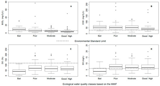
Figure 1.
Panel (A) BOD5; Panel (B) COD; Panel (C) % DO; and Panel (D) DO concentrations recorded in fresh and brackish small polder watercourses compared to the environmental standard limits of 6 mgO2/L, 30 mgO2/L, 120% and 6 mg/L (striped lines) respectively and the ecological water quality classes based on the MMIF.
Furthermore, Panel B, Figure 1, shows that almost all COD concentrations in polder watercourses were above the COD environmental standard limit of 30 mgO2/L. All the boxplots representing each of the MMIF classes are placed above the limit. Only 11.8% of the total 220 recorded values were below the standard threshold. The highest reported concentrations around 230 to 260 mgO2/L are nearly ten times higher than the acceptable standard limit.
Panel D, Figure 1, shows that in watercourses with bad ecological quality 77.8% of the 18 DO measurements in this class were below the standard limit of 6 mg/L. Regarding the poor, moderate, good and high classes it can be seen that the median of the boxplots is located slightly above the minimum required standard limit. 38.1% of the 197 recorded values distributed over these classes were reported below the standard limit. In this case only 215 measurements were available for DO concentrations. Relating panel D with C, all the DO measurements in percentage in watercourses with bad quality were below the maximum required standard limit of 120%. Whereas 14.1% of the 198 measurements recorded at poor, moderate, good high-quality classes exceed the maximum allowed percentage of DO. High percentage of oxygen measurements in these boxplots could represent oversaturated watercourses due to excessive algae growth, or high flow and turbulent waters. The, high percentage of DO encountered at watercourses with poor class could be the result of measurements taken during day light when dense aquatic plant beds produce high oxygen levels.
Altogether, boxplots in Figure 1 indicate that as lower the biological water quality in the small polder watercourses was, the higher the BOD5 concentrations and the lower DO concentration were measured. In case of COD concentrations, most of the watercourses with good and high biological water quality are just slightly above the environmental standard limit; whereas, in the other classes even higher COD concentrations were recorded.
Figure 2 shows the distribution of COD concentrations measured at effluents coming from the case study CWs, located in Gistel, Ichtegem, Langemark and Pittem (Belgium). It indicates that all of them had to deal with COD concentrations higher than the admissible discharge standard limit. Though special attention is given to the wetland located at Pittem, where most of the times the discharge standard limit was met except for two observations recorded above the 125 mgO2/L. Thus, considering these results and reported studies [39,40] we evidenced that the mitigation of COD concentrations below the discharge limit are a challenge for CWs and therefore the importance to investigate if high COD concentrations impact the ecological water quality of receiving small polder watercourses.
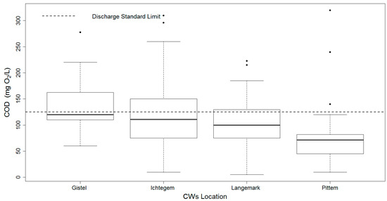
Figure 2.
COD concentrations present in the case-study CWs compared to the COD discharge standard limit of 125 mgO2/L.
3.2. MMIF and Organic Pollution Sensitive Taxa Response towards Physico-Chemical Variables
In the first stage, the systematic differences in the MMIF mean values assumed to be influenced by the sampled months and river basins were assessed by the generated linear regression model. Table 1 shows that this initial regression model, based on 207 observations, resulted in a relatively low adjusted R-squared of 0.1049; indicating that other factors may be accounted for to explain the variations or effects on the MMIF means. In addition, comparing the coefficient estimates values of each month and river basin, results indicate that those of the Brugse Polders, the Yser River basins, as well as in the month of November would pose large potential differences in the average values of the MMIF. Hence, it is concluded that there are important reasons to consider additional factors to develop an explanatory model including the sampling river basins and months in the final model specification.

Table 1.
Results of the explanatory ANOVA type approach performed to assess the differences between the means of the MMIF at each sampling river basin and month.
Subsequently, residuals were evaluated by performing a skewness/kurtosis (Jarque-Bera) test statistic which resulted on a significant skewness of 0.0136 and kurtosis of 2.3076 as shown in Table 1. It is expected that residuals with a normal distribution have a skewness of 0 and kurtosis of 3. Thus, to properly interpret results and reject or accept normality the probability skewness and kurtosis values in comparison with the probability chi-square, which indicates if the two latter violate normality, were evaluated. In this manner, the probability chi-square value of 0.0183 indicated that the null hypothesis was rejected at the 5% significance level, which strongly suggest that this initial exploratory specification is incomplete, as was originally suspected.
Table 2 indicates the resulting specification for the optimised model. It shows the final variables that can significantly explain the variance of the MMIF means with 95% confidence level. All the variables that did not significantly contribute to the overall BIC for the model fit were removed from the fully saturated model. Besides, Table 2 presents the coefficient estimates for the selected explanatory variables and their corresponding interactions influencing the MMIF means with the 95% confidence intervals. In addition, Table 2 also shows that the sample behaviour of the model residuals can be statistically classified as normally distributed though the estimated skewness (−0.273) and kurtosis (2.552) indicate a slightly longer left tail. This Gaussian distribution is justified by the probability chi-square value of 0.114 that allows the approval of the null hypothesis, in consequence the optimized model could be used for further evaluations.
Table 2.
Results of the Multivariate Linear Regression Model performed to assess the differences between the means of the MMIF and physico-chemical variables.
In that manner, by means of the coefficient estimates of the optimised regression model, the marginal or partial effects of the resulting explanatory variables over the conditional mean of the MMIF were quantified. Table 3 presents the expected partial effects of each chemical variable after the stepwise selection procedure was carried out considering the average and worst-case scenarios. The analysis of these results indicate that the positive and negative values represent the direction of the effects. On the one hand, in this case, the negative sign on the estimated marginal effects of BOD5, DO, TSS and NH4 on the average MMIF indicates that high concentrations of these variables, would lead to low mean MMIF conditions. On the other hand, the positive sign on the estimated marginal effects of COD and in some cases of DO, might be misleading if an opposite interpretation is considered. However, the positive sign indicates that most of the effect of these parameters is already captured by the BOD5 and some of the other variables and interactions that the model accommodates. In consequence, to define the variables that give information about variance in the MMIF means, it is important to consider primarily the size of the estimated effect. For instance, comparing the partial effects of COD in contrast to the ones of BOD5 and NH4, the former is four and seven times smaller respectively (in absolute terms). In general, the estimated coefficients by the developed model could be considered as a close estimation of the physico-chemical variables which could explain the variation of MMIF means under case specific conditions. Hence, the expected partial effects presented in Table 3 are not a definite indication of how much the increase or decrease of chemical concentrations would increment or lower the MMIF mean values. Rather, they serve as an indication of the relative importance each of the physico-chemical parameters has to tell about the ecological and water quality conditions. Nonetheless, by the analysis of the partial effects on the variation of the MMIF means it was seen that BOD5 captures a major part of the common effect of the studied variables, while the recalcitrant COD and the interaction among physico-chemical variables explain a minor part of the variability observed in the MMIF. Even though average and worst-case concentrations were considered, it is observed that the tendency of the effect of BOD5 remained for both situations. Only when extreme COD and TSS concentrations of (i.e., 216 mgO2/L and 80 mg/L respectively), were reported the partial effect of the BOD5 drops but not to a point higher than the one of COD.
Table 3.
Average and “worst-case” concentrations of physico-chemical variables at the polder watercourses river basins considered as input scenarios to estimate the marginal effects on the MMIF means.
Overall, the present assessment through the developed explanatory model is meant to explain the variation of the MMIF means according to different water quality conditions and thus applicable to any case-study situation. In this case, for average and assumed worst-case scenarios of polder watercourses registered between 1989 and 2015, BOD5 could be considered as an important parameter to estimate the ecological and water quality conditions, resulting in the variance of the MMIF means.
3.3. Evaluation of the Presence-Absence of Pollution Indicator Taxa
In the former section, the model developed to relate the variance in the MMIF explained by physico-chemical variables reflects a pooled response of the macroinvertebrate community towards these predictors. Therefore, masking to some extent the possibility to obtain a good estimate of the steering factors shaping the response of specific organic pollution sensitive taxa. In consequence, the following step was to inspect if there is a stronger link between the presence of specific taxa (building blocks of the MMIF) and physico-chemical parameters by means of probability linear models.
Table 4 presents the result of the selected organic pollution sensitive taxa for further evaluation. As explained in Section 2.3, this specific group of organic pollution sensitive taxa was selected based on their saprobity level and tolerance score according to the MMIF. Oligosaprobic and β-mesosaprobic taxa, living organisms tolerating BOD5 concentrations between <1 and 5 mgO2/L and NH4 concentrations between <0.1 and 0.5 mg/L with tolerance score 6 and 8, were considered as indicator organisms of organic matter pollution.
Table 4.
Organic pollution sensitive taxa to organic pollution encountered more than 20 instances from 1989–2016 in polder watercourses (Flanders–Belgium).
Later, the evaluation of their presence according to the different physico-chemical concentrations, was performed through boxplots. Figure 3 presents the concentrations at which some of the selected taxa in Table 4 are present with respect to water quality parameters (BOD5, COD, DO, TP, NO3 and TSS). The illustrated boxplots show that the selected taxa are sensitive to BOD5, NO3, DO and TSS since most of the present taxa were encountered only at concentrations lower than the environmental standard limit. However, the same trend of occurrence was not recorded in the case of COD and TP. In contrast, boxplots show that organic pollution sensitive taxa were encountered at COD and TP concentrations higher than the environmental standard limit; implying that these could have a low influence on the present taxa.
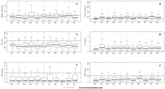
Figure 3.
Selected taxa present in the polder watercourses in relation to the environmental standard limits of Panel (A) BOD5; Panel (B) COD; Panel (C) % DO; Panel (D) TP; Panel (E) NO3; Panel (F) TSS. (Ca = Caenis, Cl = Cloeon, Gy = Gyraulus, Ha = Haliplidae, Hi = Hippeutis, Is = Ischnura, Le = Leptoceridae, Mi = Micronecta, Pl = Planorbis, Po = Potamopyrgus, Va = Valvata).
The presence/absence of the selected taxa in function of water quality parameters was evaluated through linear probability models as described in the methodology (Section 2.3). Results showed that considering the organic pollution water quality indicators, the presence of Hippeutis and Valvata was more sensitive to BOD5 concentrations; whereas, Leptoceridae’s presence was more sensitive to DO levels. Moreover, the occurrence of Caenis, Haliplidae, Micronecta, Planorbis showed to be responsive to TSS; whereas, Micronecta and Potamopyrgus’ presence was more sensitive to TP levels. A representation of the resulting model for Hippeutis after the backward selection procedure was performed, is presented in Table 5; which indicates the variables and their interactions that are significant to explain Hippeutis’ presences with a 95% confidence level. Moreover, Table 5 presents the coefficient estimates of each of these variables by which the average marginal effects on the probability of occurrence of Hippeutis were calculated.
Table 5.
Linear Probability Model developed to estimate the average marginal effects on the probability of occurrence of Hippeutis.
For further analysis, Hippeutis, Leptoceridae and Valvata were considered, since these taxa showed sensitivity to COD, BOD5 and DO which are the variables of interest in this study. In fact, among the three, only Valvata’s presence could be explained by variance in COD concentrations.
To derive final conclusions about the executed evaluation, the models’ performance of each of these taxa was assessed by computing evaluation measures derived from a confusion matrix from which four performance criteria are calculated and presented in Table 6. A confusion matrix is a two by two table presenting four outcomes produced by a binary classifier, in this case, presence–absence of the analysed taxa.
Table 6.
Different organic pollution sensitive taxa, their corresponding elements of the confusion matrices: true positive (TP), false positive (FP), false negative (FN), true negative (TN) and four different performance criteria: sensitivity (Sn), specificity (Sp), Cohen’s Kappa (Kappa) and true skill statistic (TSS). A threshold of 0.5 was used to transform probability of occurrence to presence/absence.
Results showed that considering the elements of the confusion matrix and the four different evaluation criteria, the model developed to evaluate the probability of occurrence of Leptoceridae should not be considered for further evaluation; since there was only one presence properly estimated, compared to the correct estimation of 159 absent records. In consequence, we focused on the model results of Hippeutis and Valvata. In an ecological context and following the guidelines of Manel et al. and Gabriels et al. [41,42] a Kappa statistic between 0.20–0.40 and 0.40–0.60 represent fair and moderate model performance respectively. The true skill statistic (TSS), does not have defined guidelines to classify the model performance. However, it explains the predictive accuracy of a given species distribution model based on the sensitivity and specificity. Hence, comparing the model results of the four evaluation criteria of Hippeutis and Valvata, it is concluded that the model of Valvata is better in explaining why would this taxon be absent given certain environmental conditions (COD or BOD5 concentrations), rather than being present.
This conclusion is based on the moderate model performance (Kappa = 0.52) and the slightly higher specificity (Sp = 0.83) than sensitivity (Sn = 0.69) which indicates that true-negative predictions are better estimated. In the context of defining limits, one would rather aim to get an insight of the environmental conditions when species are absent, which is in fact the reason why we considered the developed models as adequate for the present study.
Furthermore, the estimated average marginal effects given two relevant input scenarios, average and “worst-case,” are presented in Table 7. Similarly, as explained in Section 3.2, the interpretation of the estimated average marginal effects indicates that the BOD5, COD, DO, TP, NH4 and EC are correlated parameters that could indicate the ecological and water quality conditions which influence the presence of Valvata. However, BOD5 is the variable that captures most of their common effect and thus, it is an important variable that describes the impact on the probability of Valvata’s occurrence. It is important to note that the positive sign in the estimated average marginal effects indicates that the increase of the probability of occurrence of a specific taxon given one-unit increase in one of the physico-chemical variables would potentially depend on their initial value and the values of the other predictor variables. Also, the positive sign would indicate that the increase of the predictor variable would lead to the increase of the predicted probability of presence. In contrast, the negative sign would indicate that an increase of the predictor variable would lead to a decrease in the predicted probability [43].
Table 7.
Estimated average marginal effects on the probability of occurrence of organic pollution sensitive taxa given the average and “worst-case” concentrations of water quality parameters in the polder watercourses.
In this evaluation, two scenarios were considered; one regarded the average physico-chemical concentrations; and the other, considered the physico-chemical concentrations reported along with the highest COD and BOD5 recorded values. Results showed that regardless different physico-chemical conditions were considered, the trend of occurrence of Hippeutis and Valvata could be affected mainly by BOD5 concentrations. In the case of Valvata, the average marginal effect of BOD5, results from the interaction of pH, TP and TSS. The positive partial effect of 0.002 and 0.021 of COD considering average and “worst-case” conditions respectively, could be the result of the interactions among the other physico-chemical variables considered in the model. The average marginal effect of COD, results from the interaction of pH, NO3 and TSS. Hence, relating the estimated effects for BOD5 and COD with the ones of the interacting variables, one could conclude that high concentrations of TP in watercourses would influence the estimated effect in the case of BOD5, whereas, high TSS concentrations would determine a greater estimated effect in the case of COD. Nevertheless, positive and negative signs cannot always have a straightforward interpretation but is mainly the size of the effect what matters to determine the importance of the best explanatory variable.
4. Discussion
The focus of this study was to evaluate the ecological relevance of the current COD discharge standard limit for CWs treating animal manure which effluent is received in polder watercourses. In this section, two main aspects are discussed regarding the different ways physico-chemical and biological data were evaluated, to explore the significance COD as an ecological quality indicator of organic pollution. At first instance, the main drawbacks on the available data are presented with the aim to highlight important sampling criteria that should be considered in efforts of meeting specific goals, such as the EU WFD criteria. The reason this issue was taken into account relies on two points. First, that environmental limits have been usually set based on data collected mainly at large watercourses; and second that CWs effluents need to meet the same standards as other types of high-tech manure treatment installations. Then, the second aspect of discussion considered the importance of COD as indicator of organic pollution in watercourses through the interpretation of its expected partial effects in two ecological water quality indicators, the MMIF index and organic pollution sensitive taxa found in polders watercourses. Based on obtained results through the developed multivariate regression analysis and the linear probability models we evaluate if the aims of this study were met, so that alternative policy measures regarding the control of organic pollution could be formulated.
4.1. Important Criteria to Set Appropriate Environmental and Discharge Standard Limits
Even though, it is well-known that all European surface water need to meet a good ecological and water quality status regarding the EU WFD, little research or evaluations have been performed coupling the biotic and abiotic aspects in a reasonable manner. So far, there is not much evidence of ecological studies carried out, for instance, to define proper standard limits. Bio-indicators have been mainly used to determine water quality conditions. Consequently, this study is presented as a practical evaluation and illustration of setting and quantifying standard limits looking at expected variations of ecological indicators given different physico-chemical conditions.
For this analysis, a coupled data set comprised by control measurements taken on routine bases by the VMM was used. In consequence, three main downsides of the available data set are pointed out to indicate how an unsuitable assessment following generalized and standardized procedures could limit the achievement of goals. (1) Sampling periods or dates throughout the years do not always match between biotic and abiotic observations. As presented by Lock and Goethals [28], the Flemish Environment Agency has defined different sampling periods and frequencies for chemical and biological parameters; (2) Reported concentrations of the physico-chemical variables of interest (COD, BOD5 and DO) for comparison are not consistently reported or measured; (3) Sampling locations are not sequentially followed through time and space. Therefore, though the compiled data set was clustered and analysed considering different scenarios such as seasonality, type of polder waterways, sampling months and river basins to assess the ecological relevance of COD standard limit; at the end, we could only identify patterns to help steer rule setting for limits but not to ensure their relevance or to define new ones. Thus, to estimate or predict relevant abiotic-biotic coupled conditions through statistical regression analysis studies, data collected on sequential time lapses are needed. Most of the water quality assessments and standard limits delineations carried out by EU Member States are based on data gathered on a routine basis for quality control but, rather for a limited number of times data are collected based on specific objectives. Through this study, we evidenced that even though the extensive data collected on the polder watercourses, regarding physico-chemical and biological indicators for water quality conditions, statistical regression studies, can result in uncertainties or depict partial environmental or biological conditions.
In addition, another aspect to consider when it comes to discharge limits and effluent water quality control is that CWs stand under the group of manure processing plants. This implies that the different performance capacities between natural versus chemical, energy or high-technology requiring treatments are underestimated. Hence, the current COD discharge standard limit for CWs treating animal manure shown to be frequently unreachable. However, to present a consistent analysis on this matter, chronological missing data of existent biological communities in the polder watercourses and in CWs needs to be filled prior delineating suitable standard limits that can control the real impact of CWs effluents and further deterioration of the ecology of receiving watercourses.
4.2. Response of the MMIF to Physico-Chemical Variables by Means of a Multivariate Linear Model
Based on Section 4.1, the present study proceeded with the statistical analysis of the available data to determine if by this, it was possible to explain the ecological relevance of the current COD environmental and discharge standard limits imposed to for small polder watercourses and CWs treating animal manure. Bearing in mind the way data were collected, the effects of sampling periods and locations were examined by performing an exploratory ANOVA type approach. We certified that those factors were not determining an impact on the variance of the response variables but the capacity to extrapolate the results of the model to other case-study situations. Moreover, given that the good status of surface water is not only derived by controlling COD, BOD5 and DO concentrations, other variables were considered for further assessment. NO3, NH4, TP, TSS, pH and conductivity measurements are not based on the determination of oxygen levels, however, high concentrations of these in surface water could be related to organic pollution. Elevated nutrient concentrations, for example, deplete DO levels of surface water and can affect macroinvertebrates communities health [44]. Studies evaluating the relationships between water and habitat quality with macroinvertebrate communities existing in small watercourses, have considered similar variables and ways to cluster and evaluate data [44,45,46].
Therefore, by conducting statistical regression analysis we investigated if among those variables COD could be considered as a good indicator of organic pollution in relation to the ecological status and presence of macroinvertebrates species. Results concluded that COD is a variable which does not explain significantly the effect of organic pollution on ecological indicators (MMIF or organic pollution sensitive taxa) in the optimized model specification, which controls for BOD5 and other physico-chemical variables. The opposite was claimed in the case of BOD5. The hypothesis test, checking for normality in the residuals of the optimised model after the backward selection criteria was performed, allowed to conclude that the presented analysis was valid and reliable enough with a 95% confidence level. Thus, we could indicate that BOD5 is assessed as an explanatory variable which specifies better the variance in MMIF and occurrence of organic sensitive taxa. In consequence, it is proposed that one of the possible ways to assess and control organic pollution by CWs effluents, could be the re-evaluation of discharge standard limits, considering for example a (BOD5/COD) ratio adapted to the type of wastewater being treated, so that a better degree of biodegradability of organic matter could be estimated. In that manner, both water quality parameters would keep complementing to each other while major attention is given to biodegradable organic matter and not to the recalcitrant one [33,47]. Allan et al. [2] acknowledged that COD, BOD5 and BOD5/COD ratio are important water quality parameters to be considered, yet they stated that the combination of standard spot sampling techniques and laboratory analysis with emerging technologies (i.e., biomarkers or biosensors) would provide a more realistic overview of the impacts of contaminants on aquatic organisms.
In addition, rather recent studies have noted some of the limitations these two parameters present [31,48]. Apart from being the result of in spot-sampling techniques, their determination is characterized as insensitive, imprecise, time-consuming, plus chemical waste generating. Van den Broeck et al. [12] added that for the case of shallow and relatively small ponds, which represent habitat characteristics of CWs and polder water courses, climate conditions strongly determine oxygen and nutrient concentrations. Hence, snapshot measurements would disregard temporal fluctuations and as such, a proper delineation of standard environmental limits could turn out to be inadequate.
Besides, considering that CWs are aquatic macrophyte-dominated systems, where these plants and existing aquatic communities participate on the removal of organics, it is believed that the presence of recalcitrant organic matter originated by the nature of the treatment leads to high COD effluent concentrations which are not possible to degrade. In contrast, other wastewater treatment techniques use additional chemical elements, limited sets of microorganisms composed by bacteria or high inputs of energy for organic removal and thus, discharge limits could be met but in the process different compounds will be converted into products that could affect the biota.
Thus, as previously stated, the coupling of cost-effective emerging techniques (i.e., microbial bio-sensors, photometric methods, microbial biomass and microbial respiration rates to qualitatively indicate the OM content among others [48,49]) with snapshot measurements would allow a more appropriate delineation of environmental and discharge limits.
4.3. Evaluation of the Presence-Absence of Pollution Indicator Taxa
As previously stated, several studies based on the presence or ecological water quality indices of macroinvertebrates have been carried out to evaluate the ecological status of watercourses [28,44,50,51]. Some of them mainly focused on oxygen concentrations in surface water and the response of organic pollution sensitive taxa. For example, Lock et al. [28] and Connolly et al. [51] considered oxygen concentrations for modelling and predicting the presence of organic pollution sensitive taxa. On the one hand, Lock et al. [28] associated the low foreseen increase of stoneflies occurrence in watercourses in Flanders between 2015–2027, with the need of more rigorous management plans to meet the EU WFD goals. On the other hand, Connolly et al. [51], did not perceive a sensitive response on the prevalence of the macroinvertebrate communities at a mesocosm scale experiment testing low DO concentrations. Yet, they certify the need to assess the natural system and different taxa over several generations to have a more precise estimation of the effects of low DO in the biota. Yazdian et al. [45] and among others, considered DO and BOD5 as important physico-chemical variables to define biological indices.
In this study, similar aspects were replicated when the probability of occurrence of the most organic pollution sensitive taxa found in the Flemish polder watercourses was analysed. Data exploration showed that these taxa are good indicators of organic pollution given their minimal presence at low DO concentrations and high BOD5 concentrations. However, the presence of these taxa at COD concentrations higher than the environmental standard limit; and, the low estimated average effect on the occurrence probability, could be an indication that either COD cannot explain the effect of organic pollution on sensitive taxa, or that the imposed COD concentrations as standard limits do not affect their occurrence. Thus, the suggested re-evaluation of the standard thresholds or determination of alternative physico-chemical parameters concerning organic pollution levels, were supported. Considering our case study, after evaluating the effect on the probability of occurrence of organic pollution sensitive taxa present in Flemish polder watercourses, only Valvata was sensitive to COD and BOD5. However, major effect on its occurrence was detected by BOD5 than COD considering average and “worst-case” scenarios. Hence, to re-evaluate and define proper COD environmental and discharge standard limits more attention could be given to Valvata’s response towards different COD concentrations and mainly in the locations where it prevails. In fact, further research should consider the integration of abiotic and biotic components, mainly for the case of CWs. Nowadays, only few studies assessing the water and ecological quality of CWs using biological indicators in regard to the WFD have been carried out [12].
5. Conclusions
The compliance with the EU WFD goals by 2027 in EU-countries, urges policy makers and scientist to identify key ecological and water quality parameters used in combination to define the biotic and abiotic conditions of surface watercourses and setting appropriate standard limits. COD concentrations in polders watercourses located in Flanders (Belgium) are higher than the environmental standard limits. Similarly, COD concentrations determined in CWs effluents do not always meet current COD discharge criteria. Thus, we considered the importance of investigating the impact of COD on the ecology and water quality conditions of the receiving watercourses. Particularly, the relevance of COD thresholds set for the Flemish polder watercourses and CWs treating animal manure located near some of these polder watercourses, were evaluated. Different aspects were considered during the study, such as the sampling and data collection process, the performance of CWs to degrade recalcitrant organic matter and the response of biological indicators (organic pollution sensitive taxa) and ecological indices (MMIF) towards organic matter contamination quantified by COD, BOD5 and DO concentrations. Statistical regression analysis showed that higher estimated effects on the variation of the MMIF mean values and the probability of occurrence of sensitive taxa (Valvata) were given by BOD5. Given the high correlation levels present between BOD5 and COD, it is important that policies do not regard solely to current COD thresholds. The performed assessments showed, current COD standard limits in for Flemish polder watercourses and effluents coming from CWs treating animal manure do not go along with these rivers ecosystem preservation or capacity of these type of CWs to degrade recalcitrant organic matter. Considering the natural type of treatment in CWs, the presence of recalcitrant organic matter (i.e., in the form of humic substances) make COD by itself a non-sensitive parameter. In consequence, it is suggested further research to explain reliable effects of recalcitrant organic matter for this type specific scenario to define appropriate environmental limits, or to apply more sensitive legislation measures around BOD5. To this end, emerging technologies for a qualitative determination of organic matter could be tested and considered, as well as, other oxygen demand quality control parameters which are less time consuming and determined in a reliable high-throughput manner than BOD5 or COD. Besides, to define proper standard limits, models with high explanatory and predictive power need to be developed based representative ecological information in combination with abiotic data. For this, the selected sampling locations should be periodically monitored and at the same frequencies.
In any respect, a re-evaluation of the COD discharge limit would promote the implementation of CWs to treat agricultural discharges, such as liquid fractions of animal manure, which management is of big concern in Flanders and in other EU Member States.
Acknowledgments
This work was supported by the National Secretary of Higher 1217 Education, Science, Technology and Innovation (SENESCYT)–Ecuador. Open Call 2012, Second Phase. We would like to thank the Flanders Environment Agency (VMM) which provided the physico-chemical and biological data corresponding to the fresh and brackish polder watercourses running through the Flanders region. In addition, we acknowledge the support of Denis de Wilde on sample collection and chemical analysis of effluents coming from the different studied CWs in Flanders.
Author Contributions
Erik Meers and Peter L. M. Goethals conceived the performance of the present study. Natalia Donoso collected and analysed effluent water samples coming from the different wetlands. Sacha Gobeyn, Gonzalo Villa-Cox and Natalia Donoso participated in the design and development of the present research, data analysis and statistical modelling. Natalia Donoso wrote the article with collaboration and revision from Gonzalo Villa-Cox, Sacha Gobeyn, Pieter Boets, Erik Meers and Peter L. M. Goethals.
Conflicts of Interest
The authors declare no conflict of interest.
Appendix A
Table A1.
Discharge COD and BOD5 standard limits for different industrial waste water.
Table A1.
Discharge COD and BOD5 standard limits for different industrial waste water.
| Industry | Variable | |
|---|---|---|
| BOD | COD | |
| Food industry | ||
| Potato production | 25 mgO2/L | 200 mgO2/L |
| Beer and beverages industries | 25 mgO2/L | 200 mgO2/L |
| Gelatine Industry | 100 mgO2/L | 600 mgO2/L |
| Canned fruits and vegetables industries | 50 mgO2/L | 300 mgO2/L |
| Fertilizer production plants | ||
| a) Phosphate and superphosphate fertilizers, phosphoric acids and technical phosphates | Discharge into brackish surface water | |
| 25 mgO2/L | 450 mgO2/L | |
| Discharge into fresh surface water | ||
| 60 mgO2/L | 300 mgO2/L | |
| b) Nitrogen fertilizers | 50 mgO2/L | 160 mgO2/L |
| c) Fertilizers compounds | 25 mgO2/L | 150 mgO2/L |
| Manure and manure processing plants | ||
| a) Large scale installations (>60.000 ton/year) for piggery manure | 25 mg O2/L | 125 mgO2/L |
| b) All size installations for cattle production | ||
| c) Slaughterhouses | ||
| Sugar factories, juice processing raspberries and beet industries | ||
| First period Mid-September–Mid-January | 85 mgO2/L | 200 mgO2/L |
| Second period March–End May | 180 mgO2/L | 450 mgO2/L |
| Third period June–September | 30 mgO2/L | |
Table A2.
Basic water quality standards for fresh and brackish for polder surface watercourses.
Table A2.
Basic water quality standards for fresh and brackish for polder surface watercourses.
| Variable | Units | Test Indicator | Environmental Limit |
|---|---|---|---|
| EC (Fresh water) | μS/cm | 90–percentile | 1000 |
| EC (Brackish water) | μS/cm | Summer middle year average | 150,000 |
| pH (Fresh water) | pH units | Minimum–maximum | 6.5–8.5 |
| pH (Brackish water) | pH units | Minimum–maximum | 7.0–9.0 |
| Dissolved Oxygen (DO) | mgO2/L | 10–percentile | 6 |
| Dissolved Oxygen (DO) | % | Maximum | 120 |
| Total Phosphorous (TP) | mgP/L | Summer middle year average | 0.14 |
| Total Nitrogen (TN) | mgN/L | Summer middle year average | 4 |
| Nitrate (NO3) | mgN/L | 90–percentile | 5.65 |
| Total Suspended Solids (TSS) | mg/L | 90–percentile | 50 |
| Chemical Oxygen Demand (COD) | mgO2/L | 90–percentile | 30 |
| Biological Oxygen Demand (BOD5) | mgO2/L | 90–percentile | 6 |
Table A3.
Discharge standard limits for installations treating animal manure.
Table A3.
Discharge standard limits for installations treating animal manure.
| Variable | Units | Discharge Standard Limit |
|---|---|---|
| EC | μS/cm | 1000 |
| pH | pH units | 6.5–8.5 |
| Total Phosphorous (TP) | mgP/L | 2 |
| Total Nitrogen (TN) | mgN/L | 15 |
| Total Suspended Solids (TSS) | mg/L | 33 |
| Chemical Oxygen Demand (COD) | mgO2/L | 125 |
| Biological Oxygen Demand (BOD5) | mgO2/L | 25 |
| Dissolved Oxygen (DO) | mgO2/L | 6 |
Table A4.
Taxa occurring more than 20 instances indicating their saprobic and tolerance score.
Table A4.
Taxa occurring more than 20 instances indicating their saprobic and tolerance score.
| Taxa | Saprobity | Tolerance Score |
|---|---|---|
| Anisus | β-mesosaprobic | 4 |
| Armiger | β-mesosaprobic | 4 |
| Asellidae | α-mesosaprobic | 4 |
| Bithynia | β-mesosaprobic | 5 |
| Caenis | β-mesosaprobic | 6 |
| Chirnomidae-non-thummi-plumosus | β-mesosaprobic α-mesosaprobic Polysaprobic | 3 |
| Chironomidae-thummi-plumosus | β-mesosaprobic mesosaprobic Polysaprobic | 2 |
| Cloeon | β-mesosaprobic | 6 |
| Dendrocoelum | β-mesosaprobic | 5 |
| Dugesia | β-mesosaprobic | 5 |
| Dytiscidae | α-mesosaprobic | 5 |
| Erpobdella | α-mesosaprobic | 3 |
| Gammaridae | β-mesosaprobic | 5 |
| Glossiphonia | β-mesosaprobic | 4 |
| Gyraulus | Oligosaprobic β-mesosaprobic | 6 |
| Haliplidae | β-mesosaprobic | 6 |
| Helobdella | α-mesosaprobic | 4 |
| Hemiclepsis | β-mesosaprobic | 4 |
| Hippeutis | Oligosaprobic β-mesosaprobic | 6 |
| Hydracarina | Oligosaprobic | 5 |
| Ischnura | β-mesosaprobic | 6 |
| Leptoceridae | β-mesosaprobic α-mesosaprobic | 8 |
| Lymnaea | β-mesosaprobic | 5 |
| Micronecta | Oligosaprobic β-mesosaprobic | 6 |
| Naididae | β-mesosaprobic α-mesosaprobic | 5 |
| Notonecta | β-mesosaprobic | 5 |
| Palaemonidae | 5 | |
| Physa | β-mesosaprobic | 5 |
| Physella | α-mesosaprobic | 3 |
| Piscicola | β-mesosaprobic | 5 |
| Pisidium | Oligosaprobic | 4 |
| Planorbis | β-mesosaprobic | 6 |
| Potamopyrgus | β-mesosaprobic α-mesosaprobic | 6 |
| Sigara | Oligosaprobic β-mesosaprobic | 5 |
| Sphaerium | β-mesosaprobic | 4 |
| Theromyzon | β-mesosaprobic | 4 |
| Tubificidae | α-mesosaprobic | 1 |
| Valvata | β-mesosaprobic | 6 |
References
- Flanders Environment Agency (VMM). Midterm Review of the 4th Action Programme of Flanders for the Nitrates Directive Introduction; Flanders Environment Agency (VMM): Flanders, Belgium, 2013.
- Allan, I.J.; Vrana, B.; Greenwood, R.; Mills, G.A.; Roig, B.; Gonzalez, C. A “toolbox” for biological and chemical monitoring requirements for the European Union’s Water Framework Directive. Talanta 2006, 69, 302–322. [Google Scholar] [CrossRef] [PubMed]
- Donoso, N.; Boets, P.; Michels, E.; Goethals, P.L.M.; Meers, E. Environmental Impact Assessment (EIA) of Effluents from Constructed Wetlands on Water Quality of Receiving Watercourses. Water Air Soil Pollut. 2015, 226. [Google Scholar] [CrossRef]
- Gabriels, W.; Lock, K.; De Pauw, N.; Goethals, P.L.M. Multimetric Macroinvertebrate Index Flanders (MMIF) for biological assessment of rivers and lakes in Flanders (Belgium). Limnologica 2010, 40, 199–207. [Google Scholar] [CrossRef]
- Verdonschot, R.C.M.; Keizer-Vlek, H.E.; Verdonschot, P.F.M. Development of a multimetric index based on macroinvertebrates for drainage ditch networks in agricultural areas. Ecol. Indic. 2012, 13, 232–242. [Google Scholar] [CrossRef]
- Donoso, N.; Gobeyn, S.; Boets, P.; Goethals, P.L.M.; De Wilde, D.; Meers, E. Assessing the Integration of Wetlands along Small European Waterways to Address Diffuse Nitrate Pollution. Water 2017, 9, 369. [Google Scholar] [CrossRef]
- Meers, E.; Tack, F.M.G.; Tolpe, I.; Michels, E. Application of a Full-scale Constructed Wetland for Tertiary Treatment of Piggery Manure: Monitoring Results. Water Air Soil Pollut. 2008, 193, 15–24. [Google Scholar] [CrossRef]
- Boets, P.; Michels, E.; Meers, E.; Lock, K.; Tack, F.M.G.; Goethals, P.L.M. Integrated Constructed Wetlands (ICW): Ecological Development in Constructed Wetlands for Manure Treatment. Wetlands 2011, 31, 763–771. [Google Scholar] [CrossRef]
- Saeed, T.; Sun, G. A review on nitrogen and organics removal mechanisms in subsurface flow constructed wetlands: Dependency on environmental parameters, operating conditions and supporting media. J. Environ. Manag. 2012, 112, 429–448. [Google Scholar] [CrossRef] [PubMed]
- Meers, E.; Rousseau, D.P.L.; Blomme, N.; Lesage, E.; Du Laing, G.; Tack, F.M.G.; Verloo, M.G. Tertiary treatment of the liquid fraction of pig manure with Phragmites australis. Water Air Soil Pollut. 2005, 160, 15–26. [Google Scholar] [CrossRef]
- Rousseau, D.P.; Vanrolleghem, P.A.; De Pauw, N. Constructed wetlands in Flanders: A performance analysis. Ecol. Eng. 2004, 23, 151–163. [Google Scholar] [CrossRef]
- Van Den Broeck, M.; Waterkeyn, A.; Rhazi, L.; Grillas, P.; Brendonck, L. Assessing the ecological integrity of endorheic wetlands, with focus on Mediterranean temporary ponds. Ecol. Indic. 2015, 54, 1–11. [Google Scholar] [CrossRef]
- Boeuf, B.; Fritsch, O. Studying the implementation of the water framework directive in Europe: A meta-analysis of 89 journal articles. Ecol. Soc. 2016, 21. [Google Scholar] [CrossRef]
- Tachet, H.; Richoux, P.; Bournaud, M.; Usseglio-Polatera, P. Invertébrés d’eau Douce. Systématique, Biologie, Ecologiele, 1st ed.; CNRS: Paris, France, 2000. [Google Scholar]
- Flanders Environment Agency (VMM). Nutrients in Surface Water in Agricultural Area, Results MAP Measurement Network 2014-2015; Flanders Environment Agency (VMM): Flanders, Belgium, 2015. (In Dutch)
- Vlaamse Milieumaatschappij Geoviews Maps. Available online: http://geoloket.vmm.be/Geoviews/map.phtml (accessed on 28 August 2017).
- VITO EMIS (Energie-en Milieu-Informatiesysteem voor het Vlaamse Gewest). Available online: https://emis.vito.be/en/wac-2016 (accessed on 27 June 2017).
- Flemish Institute for Technological Research (VITO). Bepaling van de Elektrische Geleidbaarheid. Available online: https://esites.vito.be/sites/reflabos/2016/Online documenten/WAC_III_A_004.pdf (accessed on 9 August 2017).
- Flemish Institute for Technological Research (VITO). Bepaling van de pH. Available online: https://esites.vito.be/sites/reflabos/2016/Online documenten/WAC_III_A_005.pdf (accessed on 12 September 2017).
- Flemish Institute for Technological Research (VITO). Bepaling van Opgeloste Zuurstof. Available online: https://esites.vito.be/sites/reflabos/2016/Online documenten/WAC_III_A_008.pdf (accessed on 10 September 2017).
- Flemish Institute for Technological Research (VITO). Bepaling van Opgeloste Anionen Door Vloeistofchromatografie. Bepaling van Bromide, Chloride, Fluoride, Nitraat, Nitriet, Orthofosfaat en Sulfaat. Available online: https://esites.vito.be/sites/reflabos/2016/Online documenten/WAC_III_C_001.pdf (accessed on 13 September 2017).
- Flemish Institute for Technological Research (VITO). Bepaling Afmeting Zwevende Stoffen. Available online: https://esites.vito.be/sites/reflabos/2013/Online documenten/WAC_III_D_003.pdf (accessed on 15 December 2017).
- Flemish Institute for Technological Research (VITO). Bepaling van het Biochemisch Zuurstofverbruik (BZV) na 5 Dagen. Available online: https://esites.vito.be/sites/reflabos/2016/Online documenten/WAC_III_D_010.pdf (accessed on 15 October 2017).
- Flemish Institute for Technological Research (VITO). Bepaling van het Chemisch Zuurstofverbruik (CZV). Available online: https://esites.vito.be/sites/reflabos/2016/Online documenten/WAC_III_D_020.pdf (accessed on 8 August 2017).
- Flemish Institute for Technological Research (VITO). Bepaling van Kjeldahl-Stikstof. Methode na Mineralisatie Met Selenium. Available online: https://esites.vito.be/sites/reflabos/2016/Online documenten/WAC_III_D_030.pdf (accessed on 10 October 2017).
- Flemish Institute for Technological Research (VITO). Methoden voor de Bepaling van Kationen. Available online: https://esites.vito.be/sites/reflabos/2016/Online documenten/WAC_III_E.pdf (accessed on 10 October 2017).
- Flemish Institute for Technological Research (VITO). MMIF Berekening op Basis van op het veld Verzamelde Macro-Invertebraten. Available online: https://esites.vito.be/sites/reflabos/2016/Online documenten/WAC_V_C_002.pdf (accessed on 7 August 2017).
- Lock, K.; Goethals, P.L.M. Predicting the occurrence of stoneflies (Plecoptera) on the basis of water characteristics, river morphology and land use. J. Hydroinform. 2014, 16, 812–821. [Google Scholar] [CrossRef]
- Auvinen, H.; Du Laing, G.; Meers, E.; Rousseau, D.; Vymazal, J. Constructed wetlands treating municipal and agricultural wastewater: An overview for Flanders, Belgium. In Natural and Constructed Wetlands: Nutrients, Heavy Metals and Energy Cycling and Flow; Vymazal, J., Ed.; Springer: Cham, Switzerland, 2016; pp. 179–207. [Google Scholar]
- MACHEREY-NAGEL GmbH & Co. KG NANOCOLOR COD 160 Chemical Oxygen Dmand. Available online: ftp://ftp.mn-net.com/english/Instruction_leaflets/NANOCOLOR/985026en.pdf (accessed on 18 May 2017).
- Lee, J.; Lee, S.; Yu, S.; Rhew, D. Relationships between water quality parameters in rivers and lakes: BOD5, COD, NBOPs and TOC. Environ. Monit. Assess. 2016, 188, 252. [Google Scholar] [CrossRef] [PubMed]
- Gwaski, P.A.; Hati, S.S.; Ndahi, N.P.; Ogugbuaja, V.O. Modeling Parameters of Oxygen Demand in the Aquatic Environment of Lake Chad for Depletion Estimation. ARPN J. Sci. Technol. 2013, 3, 116–123. [Google Scholar]
- Zaher, K.; Hammam, G. Correlation between Biochemical Oxygen Demand and Chemical Oxygen Demand for Various Wastewater Treatment Plants in Egypt to Obtain the Biodegradability Indices. Int. J. Sci. Basic Appl. Res. 2014, 13, 42–48. [Google Scholar]
- Araújo, M.B.; Guisan, A. Five (or so) challenges for species distribution modelling. J. Biogeogr. 2006, 33, 1677–1688. [Google Scholar] [CrossRef]
- May, R.; Dandy, G.; Maier, H. Review of Input Variable Selection Methods for Artificial Neural Networks. In Artificial Neural Networks—Methodological Advances and Biomedical Applications; InTech: Vienna, Austria, 2011. [Google Scholar]
- Angrist, J.D.; Pischke, J.-S. Mostly Harmless Econometrics: An Empiricist’s Companion; Princeton University Press: Princeton, NJ, USA, 2008. [Google Scholar]
- Mouton, A.M.; De Baets, B.; Goethals, P.L.M. Ecological relevance of performance criteria for species distribution models. Ecol. Model. 2010, 221, 1995–2002. [Google Scholar] [CrossRef]
- Gobeyn, S.; Volk, M.; Dominguez-Granda, L.; Goethals, P.L.M. Input variable selection with a simple genetic algorithm for conceptual species distribution models: A case study of river pollution in Ecuador. Environ. Model. Softw. 2017, 92, 269–316. [Google Scholar] [CrossRef]
- Fan, J.; Wang, W.; Zhang, B.; Guo, Y.; Ngo, H.H.; Guo, W.; Zhang, J.; Wu, H. Nitrogen removal in intermittently aerated vertical flow constructed wetlands: Impact of influent COD/N ratios. Bioresour. Technol. 2013, 143, 461–466. [Google Scholar] [CrossRef] [PubMed]
- Mancilla, R.A.; Zúñiga, J.; Salgado, E.; Schiappacasse, M.C.; Chamy, R. Constructed wetlands for domestic wastewater treatment in a Mediterranean climate region in Chile. Electron. J. Biotechnol. 2013, 16. [Google Scholar] [CrossRef]
- Manel, S.; Williams, H.C.; Ormerod, S.J. Evaluating presence absence models in ecology; the need to count for prevalence. J. Appl. Ecol. 2001, 38, 921–931. [Google Scholar] [CrossRef]
- De Cooman, W.; Theuns, I.; Vos, G.; Pelicaen, J.; Maeckelberghe, H.; Gabriels, W.; Timmermans, G.; Kestens, S.; Barrez, I.; Van den Broeck, S.; et al. Milieurapport Vlaanderen, Achtergronddocument 2010, Kwaliteit Oppervlaktewater; Flanders Environment Agency (VMM): Flanders, Belgium, 2010. (In Dutch)
- UCLA: Statistical Consulting Group Probit Regression. Available online: https://stats.idre.ucla.edu/stata/output/probit-regression/ (accessed on 6 November 2017).
- Heatherly, T.; Whiles, M.R.; Royer, T.V.; David, M.B. Relationships between water quality, habitat quality and macroinvertebrate assemblages in Illinois streams. J. Environ. Qual. 2007, 36, 1653–1660. [Google Scholar] [CrossRef] [PubMed]
- Yazdian, H.; Jaafarzadeh, N.; Zahraie, B. Relationship between benthic macroinvertebrate bio-indices and physicochemical parameters of water: A tool for water resources managers. J. Environ. Heal. Sci. Eng. 2014, 12, 30. [Google Scholar] [CrossRef] [PubMed]
- Zuur, A.F.; Ieno, E.N.; Elphick, C.S. A protocol for data exploration to avoid common statistical problems. Methods Ecol. Evol. 2010, 1, 3–14. [Google Scholar] [CrossRef]
- Samudro, G.; Mangkoedihardjo, S. Review on Bod, Cod and Bod/Cod Ratio: A Triangle Zone for Toxic, Biodegradable and Stable Levels. Int. Acad. Res. 2010, 2, 235–239. [Google Scholar]
- Jouanneau, S.; Recoules, L.; Durand, M.J.; Boukabache, A.; Picot, V.; Primault, Y.; Lakel, A.; Sengelin, M.; Barillon, B.; Thouand, G. Methods for assessing biochemical oxygen demand (BOD). Water Res. 2014, 49, 62–82. [Google Scholar] [CrossRef] [PubMed]
- Nguyen, L.M. Organic matter composition, microbial biomass and microbial activity in gravel-bed constructed wetlands treating farm dairy wastewaters. Ecol. Eng. 2000, 16, 199–221. [Google Scholar] [CrossRef]
- Rizo-Patrón, V.F.; Kumar, A.; McCoy Colton, M.B.; Springer, M.; Trama, F.A. Macroinvertebrate communities as bioindicators of water quality in conventional and organic irrigated rice fields in Guanacaste, Costa Rica. Ecol. Indic. 2013, 29, 68–78. [Google Scholar] [CrossRef]
- Connolly, N.M.; Crossland, M.R.; Pearson, R.G. Effect of low dissolved oxygen on survival, emergence and drift of tropical stream macroinvertebrates. J. N. Am. Benthol. Soc. 2004, 23, 251–270. [Google Scholar] [CrossRef]
© 2018 by the authors. Licensee MDPI, Basel, Switzerland. This article is an open access article distributed under the terms and conditions of the Creative Commons Attribution (CC BY) license (http://creativecommons.org/licenses/by/4.0/).