In-Cabin Vehicle Carbon Monoxide Concentrations under Different Ventilation Settings


1
School of Population Health, University of Auckland, Private Bag 92019, Auckland 1142, New Zealand
2
Research and Investigations, Auckland Council, 135 Albert Street, Auckland 1010, New Zealand
3
School of Environment, University of Auckland, Private Bag 92019, Auckland 1142, New Zealand
4
Department of Civil and Environmental Engineering, University of Auckland, Private Bag 92019, Auckland 1142, New Zealand
*
Author to whom correspondence should be addressed.
Atmosphere 2018, 9(9), 338; https://doi.org/10.3390/atmos9090338
Submission received: 11 July 2018
/
Revised: 18 August 2018
/
Accepted: 25 August 2018
/
Published: 28 August 2018
(This article belongs to the Special Issue Impacts of Air Pollution on Human Health)
Abstract
:This paper explores the impact of choice of ventilation setting (“window open”, “new (external) air” and “recirculate”) on in-vehicle carbon monoxide exposures for commuters travelling by car at different times of the day (morning, midday, and evening) and different seasons (warm and cool) in Auckland, New Zealand. Three near-identical vehicles travelled in close proximity to each other on the same three “loops” out and into the city three times a day, each with a different ventilation setting. Concentrations of carbon monoxide were recorded using portable monitors placed inside each of the vehicles. The season was not found to be a significant factor. However, mean concentrations varied across ventilation settings by the time of day, typically peaking during the morning commute. The mean concentrations were significantly different between ventilation settings, with the recirculate setting found to result in a higher in-vehicle concentration than either new air or windows open but also heavily dependent on the initial in-vehicle concentration. However, this setting was the most effective at avoiding concentration spikes, especially when idling at intersections; an isolated peak event reaching 170 ppm was observed with the “new air” setting when following immediately behind an old, poorly-tuned, and visibly-emitting vehicle. This study suggests that having the windows open is the best setting for maintaining low in-cabin air pollution levels but that recirculate should be used in anticipation of congested conditions.
1. Introduction
Vehicle exhaust emissions make a substantial contribution towards air pollution in urban centres worldwide [1]. One of the most prominent pollutants from vehicle fuel combustion is carbon monoxide (CO). Exhaust emissions of CO can then penetrate other vehicles due to the proximity of the source and receptor and the porous nature of the vehicle envelope [2,3]. The small in-vehicle microenvironment allows for rapid increases in pollutant concentrations, and, along with long commute durations, can mean that a person’s commute can contribute disproportionately towards their daily air pollution exposure [4,5]. Also, in situations where the pollutant is being produced inside the vehicle cabin, as is the case for CO2, a pollutant buildup can occur if ventilation is not adequate [6,7].
Research both in New Zealand and elsewhere has shown that CO concentrations correlate with both NOx and ultrafine particle (UFP) (particles ≤ 0.1 µg m−3) measurements [8,9], two other prominent exhaust pollutants, suggesting that CO is useful as an indicator gas for vehicle-generated pollutants. However, CO is also an important pollutant due to its potential to lead to both long-term and short-term adverse health impacts. Short-term exposure to CO at high concentrations can cause sudden dizziness, loss of concentration, tiredness, and nausea [10,11]. The result of these effects can range from minor discomfort to vehicle occupants through to operator impairment, which can be hazardous to drivers and other road users [12]. Awareness of human health and driving impairment risks and the early availability of reliable portable air pollution monitoring technology have meant that ambient CO concentrations were amongst the first pollutants to be investigated inside vehicle cabins, with several studies carried out worldwide [10,11,13,14].
Identifying key operator behaviours in high exposure microenvironments is one way to reduce a person’s daily dose of air pollution. Studies have suggested that changing a car’s ventilation setting is one of the most influential behaviours affecting commuter exposures for car drivers [3,11,15]. Vehicular ventilation settings can be diverse in nature, and although many choices may be available, generally all ventilation settings involve the use of either fresh outdoor (new) air, a recirculating mode, or the adjustment of windows. In addition, the flow rate produced by the fan can usually be altered, artificially influencing the air exchange rate [16].
The majority of studies carried out to date investigating specifically the role of ventilation settings on in-cabin pollutant concentrations have focussed on particles, specifically UFP (particles ≤ 100 nm) [3,5,16,17]. Research into in-car air pollutant exposure when travelling through a tunnel in Sydney, Australia reported in-cabin UFP concentrations that were four to six times higher when set to “new air” than when set to recirculate [16]. However, this was within a confined outdoor setting in which pollutant concentrations can be expected to be high. Other studies carried out along major roads and motorways in the USA have shown strong inverse relationships between air exchange rates and air pollution concentrations [3]. In some studies, the reduced exposure to UFP observed when recirculating in-vehicle air was attributed to a reduction in the air exchange rate between the outdoor air and air inside the cabin when compared with using the “new air” setting [2,3,5,17]. A California motorway study of in-cabin exposure to pollution suggested that new air settings were preferable for reducing the build-up of CO2 in the cabin; it was also noted that when in a recirculation mode, UFP concentrations decreased, most likely due to the deposition of particles on interior surfaces and within the occupants’ lungs [6].
A common limitation, when considering particle pollution, is that the smallest and largest particles penetrate less efficiently due to diffusion and gravimetric deposition processes. This penetration efficiency acts to skew datasets in favour of accumulation mode particles and different particle penetration efficiencies between particle sizes [4,18]. For this reason, using a relatively inert gas such as CO can be considered a more effective metric for in-vehicle investigations of air pollution exposure.
Despite its suitability for in-vehicle exposure research, comparatively few studies investigating the effect of ventilation settings on in-cabin carbon monoxide (CO) concentrations have been undertaken. Moreover, studies have reported contradictory findings. A Hong Kong study found that air conditioning in which air was recirculated was the most effective in minimising CO exposure and showed a significantly reduced in-cabin exposure [19]. In contrast, Lebanese research reported concentrations three times higher when the ventilation was set to recirculate, and the windows closed compared to when windows were open, and 1.5 times higher compared to when it was set to “new air” and windows were kept closed [11]. A review study by Xu et al. (2018) suggests that recirculation using a high-efficiency filter is best for minimising in-cabin air pollution levels [20].
A study investigating in-cabin concentrations of CO and SO2 in Ohio, USA, found that levels depended on traffic flows and ventilation settings [21]. Several researchers have reported significant influences from meteorological conditions when investigating in-vehicle exposure [13,22]. For example, wind speed has been found to increase the air ventilation rate into the cabin whilst reducing exposure to emitted CO from nearby vehicles [15]. Traffic conditions, including on-road density and traffic flow, have also been found to significantly influence in-vehicle CO concentrations. For example, a study in Riyadh, Saudi Arabia found that a five-fold increase in traffic led to a 71% increase in in-cabin CO concentrations while a 40 km/h increase in vehicle speed reduced in-cabin concentrations by 36% [10]. The time of day has also been found to influence exposure to CO within the vehicle, with higher concentrations recorded during morning periods compared to other times of the day [13]. It is revealing that studies employing experimental and modelling research approaches have all reported correlations between external environmental variables and in-vehicle exposure [4,23]. Nevertheless, no studies have compared the role of ventilation setting under real commuting scenarios while controlling for factors such as the time of day and season. Previous studies have indicated that during periods when vehicles are stationary at intersections, concentrations of CO tend to increase, believed to be due to the closer proximity of the vehicle in front and the accumulation of pollutants over the wider intersection area due to the high density of vehicles [24].
This study attempts to identify the optimum ventilation setting by time of day (morning, midday, evening) and by season (winter and summer), while controlling for local meteorology through simultaneous measurements in both time and space, for different ventilation settings, using CO as the indicator pollutant under “real” commuting conditions. Unlike in previous studies, this paper examines the role of ventilation setting in determining in-cabin exposure under real commuting scenarios while also controlling for such factors as the time of day, season, and meteorological conditions. The results of this paper can therefore be used to advise vehicle occupants of the optimum ventilation setting for differing environments to help minimise their exposure to potentially harmful exhaust pollutants when travelling by car.
2. Methods
2.1. Geographic Setting
Auckland, New Zealand’s largest city, was chosen as the location for this study, see Figure 1. Auckland has a population of 1.4 million, covers an area of over 1000 km2, and has a sub-tropical climate. Auckland is affected by moderate levels of traffic congestion, and because no formal vehicular emission control, policy, or certification programmes exist, CO concentrations in and around major roads have been found to be relatively high at times when meteorological conditions are conducive to limited dispersion [9,25].
2.2. Experimental Routes
For this study, three commuter loops (Routes 1–3) were chosen. These routes were typical of those taken into and out of Auckland city centre. The routes are shown in Figure 1, and the average daily traffic flows of the main legs of each of the routes are presented in Table 1. Routes 1 and 2 contain sections that are motorway while all three routes contain long segments of main arterial routes. The Annual Average Daily Traffic (AADT) ranges from 88,000 vehicles on the highest volume motorway to 15,200 vehicles on the lowest volume arterial road.
2.3. Mobile CO Monitoring
Mobile CO monitoring was carried out over two one-day periods during New Zealand’s summer and winter seasons. The “summer season” trial was carried out on 28 November 2011 (three days before the official start of summer) and the “winter season” trial on 10 August 2012. Three vehicles were used in this study. The vehicles consisted of petrol-powered engines ranging in displacements from 1.3 to 2.5 L. The vehicles were of similar makes and model for both research periods. The cars used were relatively new, having been manufactured in 2010 and were less than two years old at the time of data collection. Three drivers, each in one of the vehicles, drove the pre-selected routes together; all three vehicles drove Route 1 first, then Route 2, then Route 3, with the experimental design established to replicate typical commutes to and from the Auckland central business district (CBD). A typical commute is anywhere from 10 min to 90 min depending on the distance from home to work and whether it involves travel through the centre of town, with 30 min being an average commute [26]. To investigate the personal exposure of in-vehicle commuters at different times of day, the routes were driven during the morning rush hour (07:30–09:30), the midday off-peak period (11:30–13:00), and the afternoon or evening rush hour (15:30–17:30), in local New Zealand Daylight Time (NZDT) for the summer season and New Zealand Standard Time (NZST) for the winter season for both days of monitoring. The three vehicles were driven in such a way as to remain in sight of one another, as much as traffic conditions permitted, but without travelling strictly in convoy. The combined loops took between 1.5–2 h to complete, depending on traffic conditions, and covered a total distance of about 45 km.
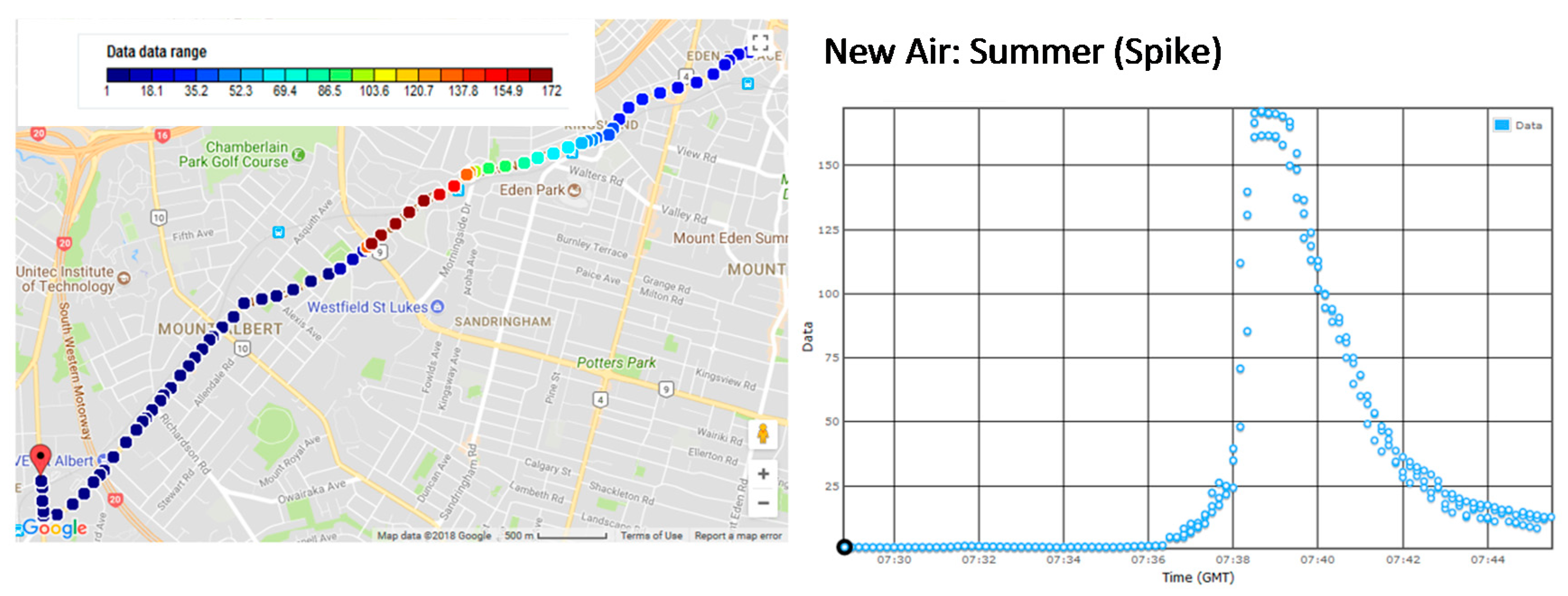
During the monitoring campaign, each driver was instructed to set their ventilation setting to either “new air (NA)”, “recirculate (RC)”, or have the active ventilation disabled and the driver’s window opened halfway, a setting called “window open (WO)”. To estimate the air exchange rate within the vehicles, the spike in concentration observed with the NA setting (discussed further later) was used in a novel way to garner a post-experimental estimate. The method of Fruin et al. [27] was utilised to determine that the air exchange rate (AER) was about 11 times per hour, see Figure S1. The WO setting would be expected to be much higher but also more dependent on the speed of travel. These ventilation settings were not altered during the monitoring periods in any way, but the different drivers/vehicles rotated ventilation settings for each of the three monitoring sessions to help control for any instrument or other driver behaviour bias, such as following distances.
The ambient 24-h CO concentrations on 28th of November were 0.4 ppm (summer average 0.55 ppm for 2011) and 0.9 ppm for the 10th of August 2012 (winter average 0.66 ppm for 2012) based on data from the Penrose Auckland fixed monitoring site. The data from this site is part of Auckland Council’s air quality monitoring network. It is categorised as a peak traffic site, located next to the Southern Motorway. The daily concentration of CO averaged annually shows traffic peaks from the same monitoring site, see Figure S2. Note that the afternoon peaks are greater than the morning. This is explained by the proximity of the monitoring station to the PM traffic heading back into Auckland. The meteorological conditions when the monitoring was conducted varied across the two seasons and for the duration of monitoring. The summer monitoring period was warmer than the winter with a maximum temperature of 22.5 °C compared to 16.9 °C. The winter monitoring sessions had lower wind speeds than the summer (averages of 1.1 (±0.85) m/s in winter and 2.4 (±1.6) m/s in summer over the monitoring periods). Notably, for the duration of the morning rush-hour period, wind speeds averaged at less than 1.3 m/s (at a height of 10 m) for both the summer and winter monitoring periods. These are based on data from two nearby meteorological stations (Penrose, close to Segment 2 on Route 20 and Pakuranga, approximately 5 km to the east of the maps presented in Figure 2).
Each vehicle was equipped with three Portable Langan T15n electrochemical sensors for monitoring CO, in addition to a GPS device. The CO sensors were co-located and subjected to a “bump test” (a range of different CO concentrations) prior to each deployment, and small linear adjustments were applied to ensure inter-instrument consistency. The sensors were programmed to log CO concentrations at a 10-s resolution and were placed on the passenger seat with the sensor exposed. Post data collection, the CO and GPS data were merged and additional metadata, such as session, traffic period, and ventilation settings were added to the database. This enabled the data to be conditioned or aggregated conveniently for analysis.
2.4. Data Conditioning
For each Langan CO monitor, the number of data points (10-s averages) collected on each run was; for the summer, 690, 480, and 780 for the morning, midday and evening, respectively; and for the winter, 683, 780, and 783 for the morning, midday and evening, respectively. Results showed the standard deviations between the three measurements were minimal, see Table 2. The highest deviation was observed for the recirculate setting during the midday run in winter. The arithmetic mean was taken from the three instruments to provide a single time series for each loop.
2.5. Statistical Analysis
Statistical analyses were carried out using IBM SPSS, Version 25. An analysis of variance was performed with the loop mean CO concentration (N = 3) as the dependent variable, and the ventilation setting (NA, RC, WO), time of day (AM, MD (midday), PM) and season (summer, winter) as the independent variables. The level of significance was set at 0.05 for all analyses.
3. Results
3.1. Time Series Data
Figure 2 shows an example of time series data for one trial (AM during the winter), for each of the three ventilation settings showing all three loops as one series. Note that the RC setting leads to more steady measurements of CO concentration compared to the other two settings. However, the initial pollution level from start-up can self-pollute at the beginning of the journey (in this case monitoring started from exiting the underground car park). Once inside, airborne pollutants can remain for extended periods when recirculating air.
3.2. Analysis of Loop Mean Concentrations
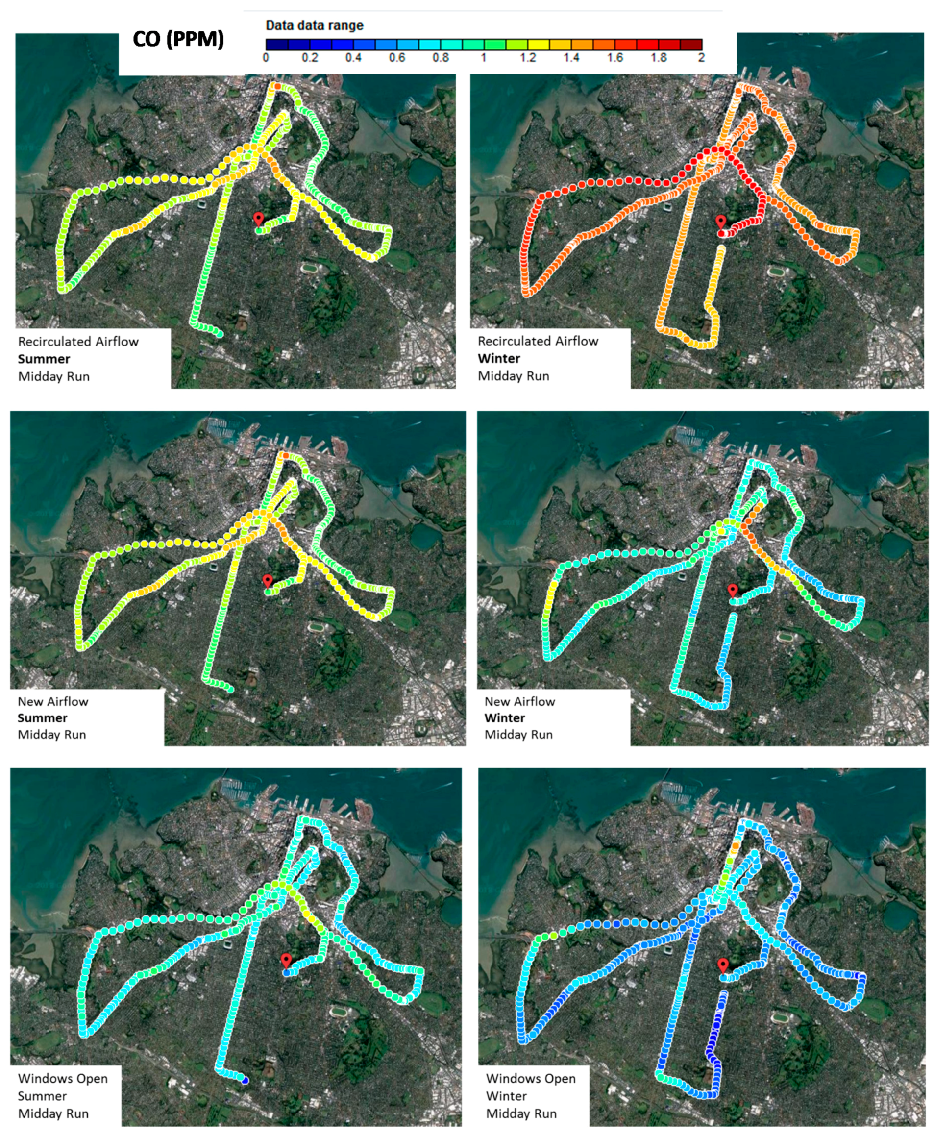
Table 3 presents the descriptive statistics for the study while Figure 3, Figure 4 and Figure 5 display the measured concentrations throughout the journeys for the three times of the day, two seasons, and three ventilation settings, based on 10-s averages. Concentrations varied in space and time with no obvious trends or locations particularly prone to high concentrations. Note that, for the morning run, in summer, and with the NA setting, an extreme short-term peak in concentration was observed. This event is discussed in more detail later but has been treated as an outlier with respect to the current results presented.
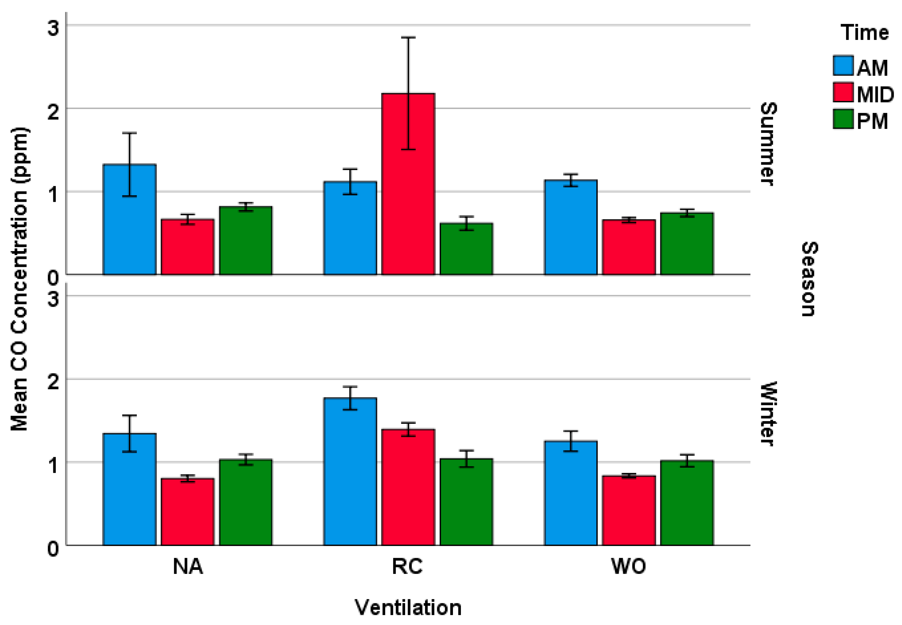
Figure 6 shows the loop mean concentration by the time of day for the three ventilation settings. The effect of ventilation setting and time of day were both found to be significant (F = 7.20, p = 0.002 and F = 7.18, p = 0.002, respectively). When considering mean concentrations for each loop with regard to seasons, the effect of season was found to be not significant (F = 2.03, p = 0.16), therefore season was removed from all subsequent analyses. Figure 7 is a bar graph of concentration by time of day and ventilation setting with both seasons combined. Table 4 shows the final analysis of variance (ANOVA) table showing that ventilation setting, time of day, and the interaction between ventilation setting and time of day are all significant (p = 0.004, p = 0.004, and p = 0.003, respectively) at the 0.05 level. The mean concentrations across all ventilation settings decreased from morning to midday to evening. The RC ventilation setting resulted in a significantly higher mean concentration than the other two settings, independent of the time of day. Post-hoc analysis suggested that the in-vehicle CO concentrations are lower for new air and windows open for the morning and midday periods, with no significant difference between settings for the evening period.
3.3. Analysis of Peak Concentrations
Analysis of the time series data identified an event, when the vehicle was stationary, that peaked at 171 ppm for a 10-s period (Figure 8), with in-vehicle concentrations taking about 11 min to decay down to median values once the vehicle began to move again, see Supporting Information, Figure S1. The peak occurred during summer data collection, in the morning, and with the ventilation set to NA. The cause of this peak in concentration was an old and poorly-tuned truck idling directly in front of the research vehicle while waiting for a traffic light to change. This event was considered an outlier for the analyses. However, the high concentration (many times greater than smoking a cigarette), could impact upon a driver’s ability to concentrate and therefore is of consequence to report [28].
4. Discussion
The highest concentrations of in-cabin CO concentrations occurred when the vehicle’s air conditioning system was set to recirculate. The key mechanism for this result appears to be the influence of pollutant infiltration upon the commencement of journeys, as illustrated in Figure 2. This is consistent with results of Esber et al. [11], who identified in-cabin CO levels in Lebanon to be higher with the ventilation set to recirculate than with the windows open. Conversely, Chan and Chung [19] report that in-cabin air was the cleanest when set to recirculate during experimentation in Hong Kong. This is also consistent with the conclusions of a review study looking across a range of pollutants [20]. It is not clear why the results contrast. However, background air pollution levels, local meteorology, vehicles fleets, driver behaviour, road types, and congestion levels are known to influence in-cabin pollution levels and may have impacted the results [5]. Indeed, the levels of congestion in the current study varied between road types, road segments, and times of the day. It is possible that the preferred ventilation setting varied depending on the vehicle speed. This was not investigated specifically but remains an area for further study.
As with many cities, traffic flows in Auckland are at their greatest during the morning period between 07:00 and 09:00 due to people commuting to workplaces and performing school runs [29]. During this period, in-vehicle concentrations were found to be at their highest. This is consistent with the results of a Californian study that reported similar traffic volumes and results in increased in-cabin exposure to traffic pollutants [4].
Driving with the windows open was found to keep CO levels within the car at their lowest level when compared with other ventilation settings. This is most likely due to a rapid air exchange rate between in-vehicle and outdoor air, which can be considered largely clean when not drawing mechanically from the front of the car and therefore receiving exhaust pollutants from vehicles directly in front. Indeed, it was the period when the experimental car was following a poorly maintained truck with ventilation set to new air that a large spike in concentration occurred. Although an isolated event during the period of experimentation, it does point to the risk associated with using this setting. Moreover, the 10-min decay curve after the peak in CO shows that the influx of pollutants through the new air setting can be persistent, amplifying the associated possible health outcomes.
Previous work carried out in Nottingham in the United Kingdom [24] describes recorded peak concentrations of in-cabin concentrations as a direct response to the emissions of nearby vehicles. The results highlight the importance of ensuring that the air inside the vehicle is clean before setting the ventilation to recirculate as the rate of air exchange is low, allowing pollutants to remain within the cabin. There is also the potential for CO2 to accumulate inside vehicles when air is set to recirculate [6,7], especially if the occupancy-to-volume ratio is high.
When the air ventilation was set to recirculate, it was observed that CO concentrations tended to be higher at the beginning of the run, and then reduced as the car progressed along the three routes. Although uncertain, this may be attributed to the cold engine at the start of the journey; catalytic converters fitted into cars to transform CO to CO2 are less effective when cold, releasing more CO upon starting the vehicle’s engine [30].
The main limitation of this study was that it consisted of only one day of field trials for each season. However, given that simultaneous measurements were made, the day-to-day variability in concentrations due to weather and other factors can to some extent be eliminated. Also, three “independent” loops were driven, allowing some modest statistical analysis to be carried out and conclusions made, though limited in their degree of robustness. Different conclusions may have been made had sampling occurred during a day of high outdoor ambient levels rather than days more typical of the season.
Additionally, considerations were not given to the impact of the following distance to the vehicle in front, and the impact this might have on in-vehicle concentrations, especially for the window open and new air settings. This is left for future investigation.
5. Conclusions
This paper describes in-vehicle CO concentrations in three separate, but near-identical vehicles, driven during three different times of day along three different loops out of the city centre and back in, during the summer and winter seasons in Auckland. Three different ventilation settings were tested including “windows open”, “new air”, and “recirculate”. The results demonstrate that the mean in-cabin concentrations vary little by season but vary by time of day; specifically, average levels are higher in the morning compared with other times of the day. To minimise in-cabin exposure, the recirculate setting should be avoided during the morning and midday periods in particular, in preference of open windows. Concentrations vary considerably over time for the new air and window open settings due to the high air exchange rates associated with these settings compared to the recirculate setting. Therefore, to avoid short-term spikes in concentration (as was observed in an isolated event in the current study), it is recommended that the new air not be used in congested conditions as the close proximity to the car in front makes a vehicle susceptible to spikes in concentration that can be avoided by opening a window instead.
Supplementary Materials
The following are available online at https://www.mdpi.com/2073-4433/9/9/338/s1, Figure S1 Time series data from an on-road spike to estimate the vehicle ventilation rate during new air ventilation setting during morning commute, Figure S2: Annual averaged 24-h CO data collected from Penrose air quality monitoring station.
Author Contributions
Conceptualization, K.N.D., J.A.S. and S.B.C.; Methodology, K.N.D., J.A.S. and S.B.C., Data Analysis, N.P.T. and K.N.D.; Writing-Original Draft Preparation, K.N.D. and N.P.T.; Writing-Review & Editing, J.A.S., and S.B.C.
Funding
This research received no external funding.
Acknowledgments
Lucy Ferris and Rosalind Payne are thanked for their help with data collection and preliminary analysis of part of the data. Stuart Grange is also thanked for help with the compilation of the data in the early stages of the project.
Conflicts of Interest
The authors declare no conflict of interest.
References
- Mayer, H. Air Pollution in Cities. Atmos. Environ. 1999, 33, 4029–4037. [Google Scholar] [CrossRef]
- Zhu, Y.; Hinds, W.C.; Krudysz, M.; Kuhn, T.; Froines, J.; Sioutas, C. Penetration of freeway ultrafine particles into indoor environments. J. Aerosol Sci. 2005, 36, 303–322. [Google Scholar] [CrossRef]
- Hudda, N.; Fruin, S.A. Models for predicting the ratio of particulate pollutant concentrations inside vehicles to roadways. Environ. Sci. Technol. 2013, 47, 11048–11055. [Google Scholar] [CrossRef] [PubMed]
- Li, L.; Wu, J.; Hudda, N.; Sioutas, C.; Fruin, S.A.; Delfino, R.J. Modeling the concentrations of on-road air pollutants in Southern California. Environ. Sci. Technol. 2013, 47, 9291–9299. [Google Scholar] [CrossRef] [PubMed]
- Hudda, N.; Kostenidou, E.; Sioutas, C.; Delfino, R.J.; Fruin, S.A. Vehicle and driving characteristics that influence in-cabin particle number concentrations. Environ. Sci. Technol. 2011, 45, 8691–8697. [Google Scholar] [CrossRef] [PubMed]
- Zhu, Y.; Eiguren-Fernandez, A.; Hinds, W.C.; Miguel, A.H. In-cabin commuter exposure to ultrafine particles on Los Angeles Freeways. Environ. Sci. Technol. 2007, 41, 2138–2145. [Google Scholar] [CrossRef] [PubMed]
- Jung, H. Modelling CO2 Concentrations in Vehicle Cabin; SAE International: Warrendale, PA, USA, 2013. [Google Scholar] [CrossRef]
- Chan, A. Indoor–outdoor relationships of particulate matter and nitrogen oxides under different outdoor meteorological conditions. Atmos. Environ. 2002, 36, 1543–1551. [Google Scholar] [CrossRef]
- Dirks, K.N.; Sharma, P.; Salmond, J.A.; Costello, S.B. Personal exposure to air pollution for various modes of transport in Auckland, New Zealand. TOASJ 2012, 6, 84–92. [Google Scholar] [CrossRef]
- Koushki, P.A.; Al-Dhowalia, K.H.; Niaizi, S.A. Vehicle occupant exposure to carbon monoxide. J. Air Waste Manag. Assoc. 1992, 42, 1603–1608. [Google Scholar] [CrossRef]
- Esber, L.A.; El-Fadel, M.; Nuwayhid, I.; Saliba, N. The effect of different ventilation modes on in-vehicle carbon monoxide exposure. Atmos. Environ. 2007, 41, 3644–3657. [Google Scholar] [CrossRef]
- Weichenthal, S.; Van Ryswyk, K.; Kulka, R.; Sun, L.; Wallace, L.; Joseph, L. In-vehicle exposures to particulate air pollution in Canadian metropolitan areas: The urban transportation exposure study. Environ. Sci. Technol. 2015, 49, 597–605. [Google Scholar] [CrossRef] [PubMed]
- Alm, S.; Jantunen, M.J.; Vartiainen, M. Urban commuter exposure to particle matter and carbon monoxide inside an automobile. J. Expo. Anal. Environ. Epidemiol. 1999, 9, 237. [Google Scholar] [CrossRef] [PubMed]
- Saksena, S.; Prasad, R.K.; Shankar, V.R. Daily exposure to air pollutants in indoor, outdoor and in-vehicle micro-environments: A pilot study in Delhi. Indoor Built Environ. 2007, 16, 39–46. [Google Scholar] [CrossRef]
- Zagury, E.; Le Moullec, Y.; Momas, I. Exposure of Paris taxi drivers to automobile air pollutants within their vehicles. Occup. Environ. Med. 2000, 57, 406–410. [Google Scholar] [CrossRef] [PubMed] [Green Version]
- Knibbs, L.D.; de Dear, R.J.; Morawska, L. Effect of cabin ventilation rate on ultrafine particle exposure inside automobiles. Environ. Sci. Technol. 2010, 44, 3546–3551. [Google Scholar] [CrossRef] [PubMed]
- Hill, L.B.; Gooch, J. A Multi-City Investigation of Exposure to Diesel Exhaust in Multiple Commuting Modes; CATF Special Report 2007-1; Clean Air Task Force: Boston, MA, USA, 2007. [Google Scholar]
- Nazaroff, W.W. Indoor particle dynamics. Indoor Air 2004, 14 (Suppl. 7), 175–183. Available online: http://escholarship.org/uc/item/80f883g7 (accessed on 4 December 2015). [CrossRef] [PubMed] [Green Version]
- Chan, A.T.; Chung, M.W. Indoor–outdoor air quality relationships in vehicle: Effect of driving environment and ventilation modes. Atmos. Environ. 2003, 37, 3795–3808. [Google Scholar] [CrossRef]
- Xu, B.; Chen, X.; Xiong, J. Air quality inside motor vehicles. Indoor Built Environ. 2018, 27, 452–465. [Google Scholar] [CrossRef]
- Kadiyala, A.; Kumar, A. Study of in-vehicle pollutant variation in public transport buses operating on alternative fuels in the city of Toledo, Ohio. Open Environ. Biol. Monit. J. 2011, 4, 1–20. [Google Scholar] [CrossRef]
- Flachsbart, P.G. Models of exposure to carbon monoxide inside a vehicle on a Honolulu highway. J. Expo. Anal. Environ. Epidemiol. 1999, 9, 245–260. [Google Scholar] [CrossRef] [PubMed] [Green Version]
- Kingham, S.; Longley, I.; Salmond, J.; Pattinson, W.; Shrestha, K. Variations in exposure to traffic pollution while travelling by different modes in a low density, less congested city. Environ. Pollut. 2013, 181, 211–218. [Google Scholar] [CrossRef] [PubMed]
- Clifford, M.J.; Clarke, R.; Riffat, S.B. Drivers’ exposure to carbon monoxide in Nottingham, U.K. Atmos. Environ. 1997, 31, 1003–1009. [Google Scholar] [CrossRef]
- Coulson, G.; Olivares, G.; Talbot, N. Aerosol Size Distributions in Auckland. Air Qual. Clim. Chang. 2016, 50, 23–28. [Google Scholar]
- NZAVS Policy Brief Regional Commute Times. Available online: https://cdn.auckland.ac.nz/assets/psych/about/our-research/nzavs/Feedback%20Reports/NZAVS-Policy-Brief-Regional-Commute-Times.pdf (accessed on 15 August 2018).
- Fruin, S.A.; Hudda, N.; Sioutas, C.; Delifino, R.J. A predictive model for vehicle air exchange rates based on a large, representative sample. Environ. Sci. Technol. 2011, 45, 3569–3575. [Google Scholar] [CrossRef] [PubMed]
- Kaur, S.; Nieuwenhuijsen, M.; Colvile, R. Fine particulate matter and carbon monoxide exposure concentrations in urban street transport microenvironments. Atmos. Environ. 2007, 41, 4781–4810. [Google Scholar] [CrossRef]
- Auckland Council. Traffic Count Data. Published 2014. Available online: https://at.govt.nz/about-us/reports-publications/traffic-counts/ (accessed on 11 July 2018).
- Marlow, D. Evaluation of Carbon Monoxide Concentration with and without Catalytic Emission Controls from Gasoline Propulsion Engines; Report Number EPHB 289-12a; U.S. Department of Health and Human Services: Washington, DC, USA, 2007.
Figure 1.
Maps of the three different transit routes across Auckland. Images taken from Google Maps.
Figure 1.
Maps of the three different transit routes across Auckland. Images taken from Google Maps.
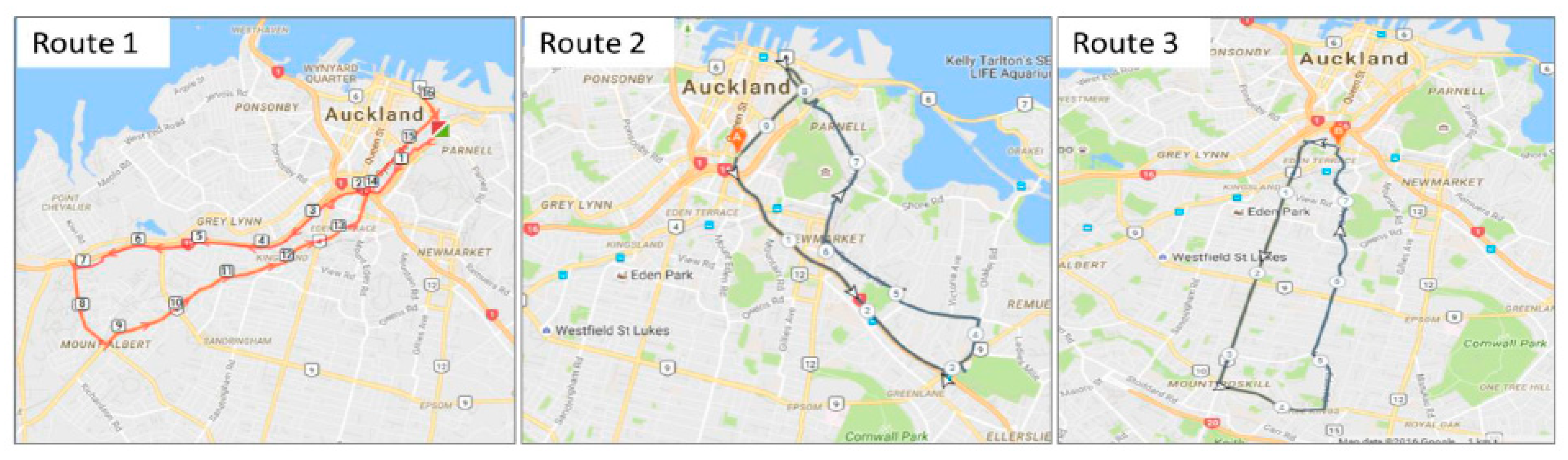
Figure 2.
Examples of time series data for two trials. AM during the summer (a) and AM for winter (b) for each of the three ventilation settings showing all three loops as one series.
Figure 2.
Examples of time series data for two trials. AM during the summer (a) and AM for winter (b) for each of the three ventilation settings showing all three loops as one series.
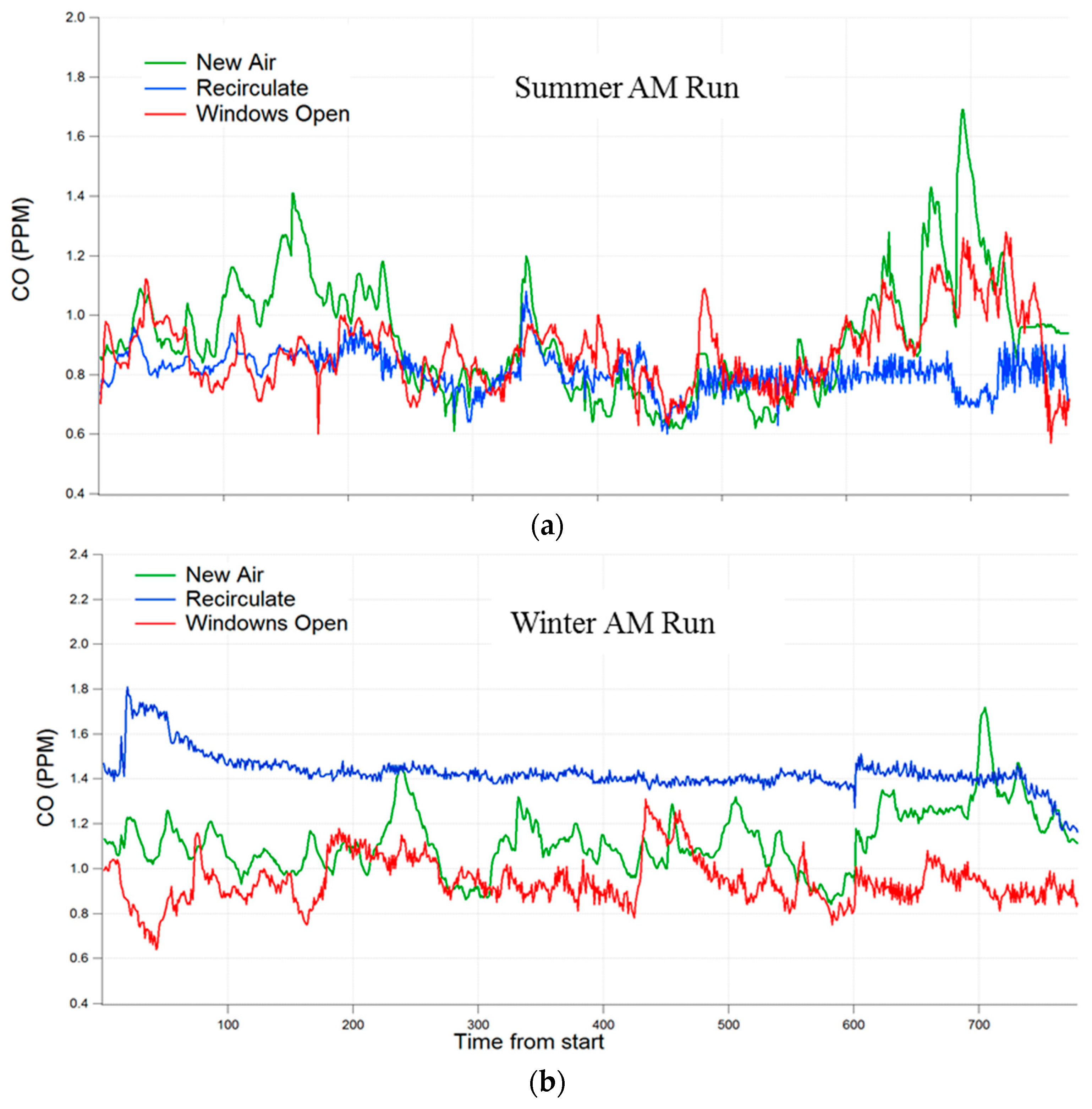
Figure 3.
Morning 10-s averaged CO concentrations. Data from the summer on the left and winter on the right. The ventilations settings are: “Recirculate” (top), “new air” (middle), and “windows open” (bottom). The CO ppm range is shown in the legend at the top of the first graph and is consistent throughout the three graphs.
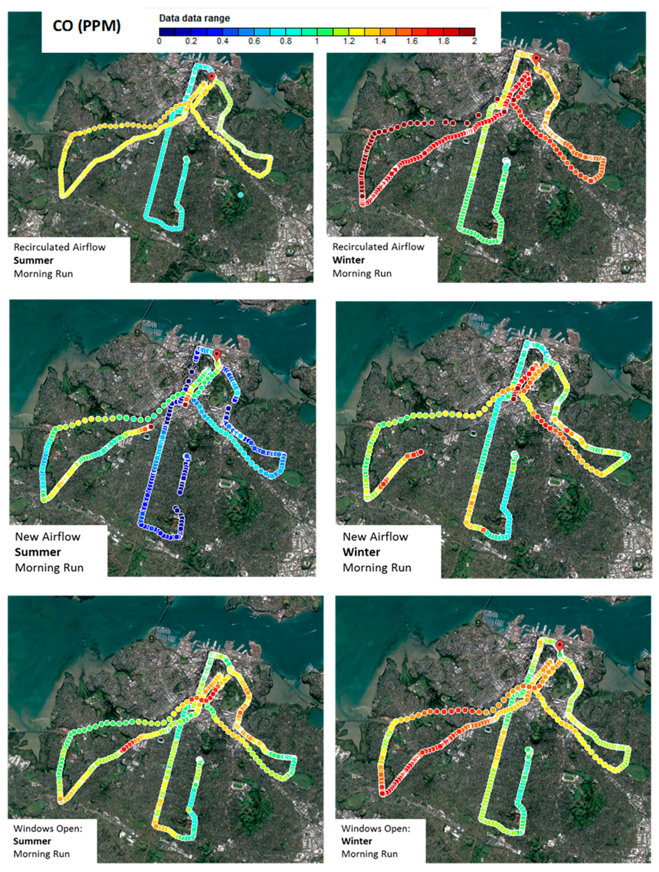
Figure 4.
Off-peak “midday” 10-s averaged CO concentrations. Data from the summer on the left and winter on the right. The ventilations settings are: “Recirculate” (top), “new air” (middle), and “windows open” (bottom). The CO ppm range is shown in the legend at the top of the first graph and is consistent throughout the three graphs.

Figure 5.
Afternoon 10-s averaged CO concentrations. Data from the summer on the left and winter on the right. The ventilations settings are: “Recirculate” (top), “new air” (middle), and “windows open” (bottom). The CO ppm range is shown in the legend at the top of the first graph and is consistent throughout the three graphs.
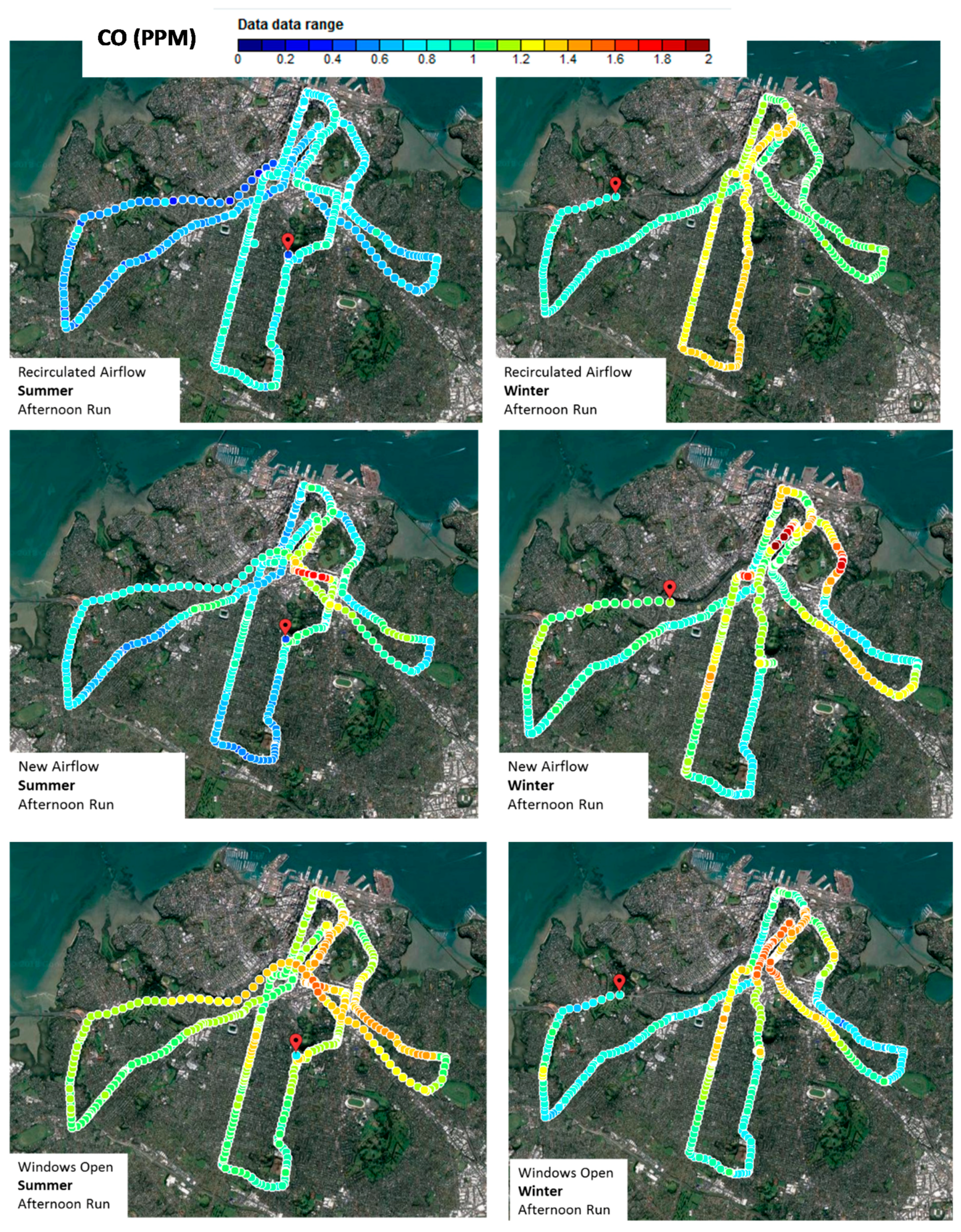
Figure 6.
Bar graph showing the loop mean concentrations for each of the periods of monitoring sorted by season. The error bars represent one standard error of the mean (N = 3).
Figure 6.
Bar graph showing the loop mean concentrations for each of the periods of monitoring sorted by season. The error bars represent one standard error of the mean (N = 3).

Figure 7.
Bar graph showing the loop mean concentrations for each of the periods of monitoring with both seasons combined. The error bars represent one standard error of the mean (N = 6).
Figure 7.
Bar graph showing the loop mean concentrations for each of the periods of monitoring with both seasons combined. The error bars represent one standard error of the mean (N = 6).
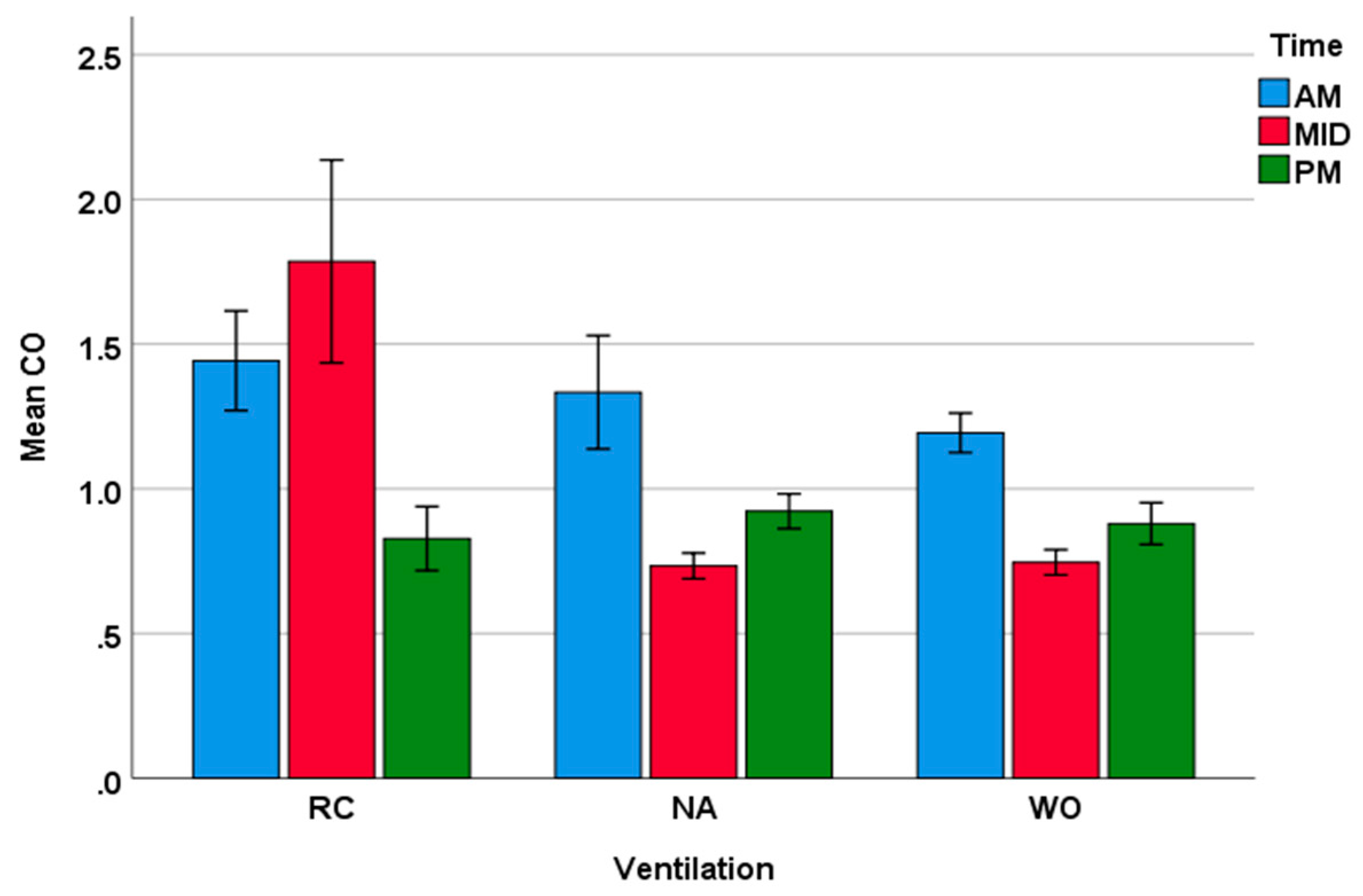
Figure 8.
Time series of air pollution concentration showing a very intense peak observed during the summer morning commute when the vehicle was set to new air (NA). Note that the concentrations reach levels in excess of 170 ppm for a short period.
Figure 8.
Time series of air pollution concentration showing a very intense peak observed during the summer morning commute when the vehicle was set to new air (NA). Note that the concentrations reach levels in excess of 170 ppm for a short period.

Table 1.
Average daily number of vehicles per day and their associated route segments for each of the routes presented in Figure 1.
Table 1.
Average daily number of vehicles per day and their associated route segments for each of the routes presented in Figure 1.
| Route | Road Name | Approximate Segment Range (km) | Average Daily Traffic Count (Vehicles per Day) |
|---|---|---|---|
| Route 1 | SH 16 (Motorway) | 1–7 | 58,000 |
| Great North Road | 7–9 | 16,000 | |
| New North Road | 9–16 | 19,000 | |
| Route 2 | SH 1 (Motorway) | 9–3 | 88,000 |
| Remuera Road | 3–6 | 23,400 | |
| Parnell Road | 6–8 | 18,800 | |
| Upper Queen Street | 8–9 | 17,700 | |
| Route 3 | Dominion Road | 1–3 | 25,900 |
| Balmoral Road | 4 | 24,100 | |
| Mt Eden Road | 5–8 | 15,200 |
Table 2.
Average standard deviation between the three sensors deployed for each of the ventilation settings, season, and time of day based on 10-s averages: RC (recirculate), WO (window open), NA (new air).
Table 2.
Average standard deviation between the three sensors deployed for each of the ventilation settings, season, and time of day based on 10-s averages: RC (recirculate), WO (window open), NA (new air).
| Ventilation | RC AM | RC MID | RC PM | WO AM | WO MID | WO PM | NA AM | NA MID | NA PM |
|---|---|---|---|---|---|---|---|---|---|
| St Dev Summer (ppm) | 0.006 | 0.095 | 0.131 | 0.016 | 0.142 | 0.078 | 0.059 | 0.095 | 0.074 |
| St Dev Winter (ppm) | 0.024 | 0.216 | 0.077 | 0.031 | 0.135 | 0.031 | 0.092 | 0.062 | 0.074 |
Table 3.
Descriptive statistics. The arithmetic means and standard deviations (St Dev) are based on the loop averages (n = 3) for a time of day, season, and ventilation setting.
Table 3.
Descriptive statistics. The arithmetic means and standard deviations (St Dev) are based on the loop averages (n = 3) for a time of day, season, and ventilation setting.
| Season | Ventilation | Morning | Midday | Evening | |||
|---|---|---|---|---|---|---|---|
| Mean (ppm) | St Dev (ppm) | Mean (ppm) | St Dev (ppm) | Mean (ppm) | St Dev (ppm) | ||
| Winter | RC | 1.77 | 0.24 | 1.39 | 0.14 | 1.04 | 0.17 |
| NA | 1.34 | 0.38 | 0.80 | 0.68 | 1.03 | 0.11 | |
| WO | 1.25 | 0.21 | 0.84 | 0.04 | 1.02 | 0.13 | |
| Summer | RC | 1.12 | 0.26 | 2.18 | 1.17 | 0.62 | 0.14 |
| NA | 1.32 | 0.66 | 0.67 | 0.10 | 0.81 | 0.08 | |
| WO | 1.13 | 0.12 | 0.66 | 0.05 | 0.74 | 0.07 | |
Table 4.
Final analysis of variance (ANOVA) Table showing degrees of freedom (Df) mean square (MS), variance (F) and significance (Sig).
Table 4.
Final analysis of variance (ANOVA) Table showing degrees of freedom (Df) mean square (MS), variance (F) and significance (Sig).
| Source | Squares | Df | MS | F | Sig |
|---|---|---|---|---|---|
| Ventilation | 1.799 | 2 | 0.899 | 6.121 | 0.004 |
| Time | 1.795 | 2 | 0.898 | 6.110 | 0.004 |
| Ventilation × Time | 2.792 | 4 | 0.698 | 4.750 | 0.003 |
| Error | 6.611 | 45 | 0.147 |
© 2018 by the authors. Licensee MDPI, Basel, Switzerland. This article is an open access article distributed under the terms and conditions of the Creative Commons Attribution (CC BY) license (http://creativecommons.org/licenses/by/4.0/).
Share and Cite
MDPI and ACS Style
Dirks, K.N.; Talbot, N.; Salmond, J.A.; Costello, S.B. In-Cabin Vehicle Carbon Monoxide Concentrations under Different Ventilation Settings. Atmosphere 2018, 9, 338. https://doi.org/10.3390/atmos9090338
AMA Style
Dirks KN, Talbot N, Salmond JA, Costello SB. In-Cabin Vehicle Carbon Monoxide Concentrations under Different Ventilation Settings. Atmosphere. 2018; 9(9):338. https://doi.org/10.3390/atmos9090338
Chicago/Turabian StyleDirks, Kim N., Nicholas Talbot, Jennifer A. Salmond, and Seosamh B. Costello. 2018. "In-Cabin Vehicle Carbon Monoxide Concentrations under Different Ventilation Settings" Atmosphere 9, no. 9: 338. https://doi.org/10.3390/atmos9090338
Note that from the first issue of 2016, this journal uses article numbers instead of page numbers. See further details here.