Article

Dynamic Ensemble Analysis of Frontal Placement Impacts in the Presence of Elevated Thunderstorms during PRECIP Events

1
Cooperative Institute for Research in the Environmental Sciences, University of Colorado, Boulder, CO 80309, USA
2
Weather Prediction Center, 5830 University Research Court, College Park, University of Maryland, College Park, MD 20740, USA
3
Atmospheric Science Program, School of Natural Resources, University of Missouri, Columbia, MO 65211, USA
*
Author to whom correspondence should be addressed.
Atmosphere 2018, 9(9), 339; https://doi.org/10.3390/atmos9090339
Submission received: 30 May 2018 / Revised: 17 August 2018 / Accepted: 26 August 2018 / Published: 29 August 2018
(This article belongs to the Special Issue Precipitation: Measurement and Modeling)

Abstract

:
The Program for Research on Elevated Convection with Intense Precipitation (PRECIP) field campaign sampled 10 cases of elevated convection during 2014 and 2015. These intense observing periods (IOP) mostly featured well-defined stationary or warm frontal zones, over whose inversion elevated convection would form. However, not all frontal zones translated as expected, with some poleward motions being arrested and even returning equatorward. Prior analyses of the observed data highlighted the downdrafts in these events, especially diagnostics for their behavior: the downdraft convective available potential energy (DCAPE) and the downdraft convective inhibition (DCIN). With the current study, the DCAPE and DCIN are examined for four cases: two where frontal motion proceeded poleward, as expected, and two where the frontal motions were slowed significantly or stalled altogether. Using the Weather Research and Forecasting (WRF) model, a multi-model ensemble was created for each of the four cases, and the best performing members were selected for additional deterministic examination. Analyses of frontal motions and surface cold pools are explored in the context of DCAPE and DCIN. These analyses further establish the DCAPE and DCIN, not only as a means to classify elevated convection, but also to aid in explaining frontal motions in the presence of elevated convection.

1. Introduction

Elevated thunderstorm complexes pose numerous threats and are well established as producers of heavy rainfall [1,2,3,4], flash flooding [3,4,5], and cloud-to-ground lightning flashes [4,6,7]. Furthermore, these elevated complexes are suspected of disrupting synoptic boundary location and movement [8,9] as cold pools from convection interact with surface boundaries. This paper will show that not all low-level stable layers are impenetrable. It will be shown that it is possible in certain environments for downdrafts from elevated convection to penetrate through weak low-level stable layers and impact surface weather by bringing potentially colder air down. Understanding what conditions cause frontal displacement to happen or not happen is a worthwhile pursuit, as it could lead to a better, more timely forecasting of heavy rains. Such storms were sampled during the Program for Research on Elevated Convection with Intense Precipitation (PRECIP) field campaigns during the warm seasons of 2014–2015.
During the PRECIP campaigns, it was observed several times that convection north of a boundary would cause the boundary to stall and retrograde against its prior advancement as cold pools unified and spread in the direction of the advancing front. When this was observed, heavy precipitation occurred where the front and cold pools were interacting. This phenomena did not occur during every instance of observed elevated convection. It was noted that when elevated convection retained a more cellular radar appearance, boundaries were not observed to stall.
Market et al. [10] introduced the concept of downdraft convective inhibition (DCIN) and its potential utility when compared to downdraft convective available potential energy (DCAPE). They explained that DCIN is akin to the negative area above the equilibrium level that is used to estimate the height of the overshooting top of a cumulonimbus, but when applied to DCAPE, where the equilibrium level is at the top of the DCIN layer for a descending parcel in a sounding. Market et al. [10] stated that as DCIN becomes progressively larger in comparison with the DCAPE, it is progressively more difficult for a downdraft to penetrate down toward the surface; these are the conditions where DCIN > DCAPE further confine near-surface parcels to the subinversion layer. This was found to be the delineating factor in the PRECIP cases that examined which boundaries stalled and those that did not. It is therefore thought to be a main contributor to frontal stalling.

2. Background and Discussion

2.1. Defining Elevated Convection

Colman [11,12] established one definition of elevated convection as a storm that is isolated from surface diabatic effects and found above a frontal inversion. He further refined this definition to include that observations must lie on the cold side of an analyzed front with clear contrast in the mass and momentum fields with surrounding stations recording similar conditions. Similar criteria were also used by Grant [13], Rochette and Moore [1], Moore et al. [14], Moore et al. [3], and McCoy et al. [4] for studies involving elevated thunderstorms. However, this definition is rather specific, and, while being useful in determining if a given cell is surface-based or elevated by way of synoptic map interrogation, it falls short in defining elevated convection in scenarios where a boundary is not well-defined. Indeed, there have been valid concerns about how to assess whether deep moist convection is purely elevated [15]. In their earlier work, Corfidi et al. [16] explained that surface-based convection will often incorporate elevated parcels, and that elevated convection can also include surface parcels into its updraft. These facts can blur the line between what is elevated convection and what is surface-based convection, and it becomes especially hard to distinguish as convection transitions from surface-based to elevated and vice versa. A more applicable definition was proposed by Corfidi et al. [16] in which elevated thunderstorms are defined as convection occurring over a stable layer near the surface, which is essentially cut off from surface-based instability. Certainly, convection can be elevated even when near-surface parcels have positive CAPE, as suggested by Nowotarski et al. [17]. Thus, many of the cases sampled during PRECIP, of which all were north of a boundary, fall into the category of mostly elevated convection, but perhaps not all of them were purely elevated.
The study below will analyze convective environments that show both purely and hybrid elevated convective environments [18]. While the general hazards of thunderstorms are similar for both environments [5,6], contrasting the evolution of the environment and differing characteristics of the systems that evolve are important findings of this study.

2.2. Forecasting Elevated Convection and Cold Pools

Forecasting the evolution and movement of elevated complexes and the impacts to the surrounding environment has been a struggle for forecasters [8,19] and numerical weather prediction (NWP) models [15,19,20] alike. One of the primary causes of this complexity is how cold pools from thunderstorms interact with the surrounding environment [20,21]. Cold pools are generated as rain evaporates into dry air, and by downdrafts introducing cooler, drier air from aloft [22]. It is well-established that thunderstorms are often generated or enhanced at the leading edge of the gust front [20,21,23,24,25]. It has been shown that cells forming along and behind the gust front can form as high as 2 km above the depth of the cold pool [24], thus making these new cells potentially elevated. It has also been demonstrated that cold pools with a larger temperature deficit than their environment produced deeper cold pools with more lift [23]. The location, depth, and longevity of cold pools can have dramatic impacts on how much rain is able to be produced and sustained [19].

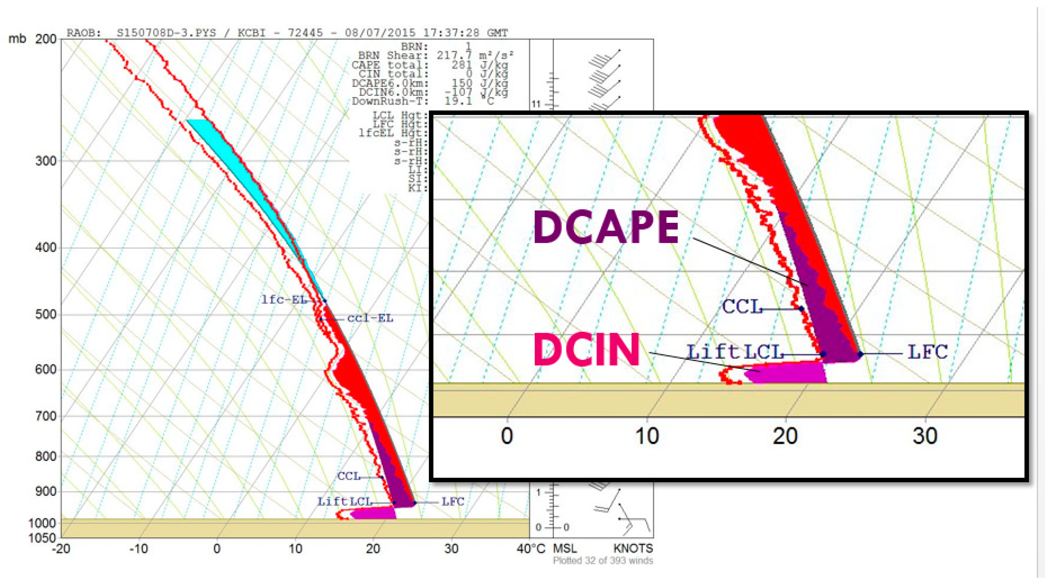
2.3. Defining DCIN and DCAPE

DCIN and DCAPE are crucial elements to this work and will be defined below. DCAPE represents the potential for a downdraft to penetrate the near-surface stable layer. This study will use the Market et al. [10] definition used for elevated convection:
DCAPE = g   Z n b Z n θ v ( z ) θ v v ( z ) θ v ( z ) d z
where θ v ( z ) and θ v ( z ) are the virtual potential temperatures of the environment and saturated downdraft parcels, respectively. Z n is the height where the parcel begins descending, and Z n b is the level of neutral buoyancy. The lower bound of the integral, Z n b , is the significant change when we consider the presence of a near-surface stable layer and inversion that can act to slow or stop a downdraft’s descent. DCAPE represents the negative buoyancy of a parcel with the saturated downdraft. DCAPE has commonly been discussed in the framework of surface-based convection, with the assumption that the downdraft will travel down to the surface unabated.
In some elevated convective environments, this assumption may not necessarily hold true. As Market et al. [10] stated, a negative area on a thermodynamic diagram can be represented for the downrushing parcel that becomes warmer than its environment in the near-surface stable layer. This quantity is labeled DCIN, and is represented mathematically as:
DCIN = g   Z s f c Z n b θ v ( z ) θ v v ( z ) θ v ( z ) d z
This expression’s components are identical to those of DCAPE, expect for the limits of integration, which are Z n b as above, and the surface of the earth, Z s f c . Examples of DCIN within an observed sounding and as a gridded field are provided below. DCAPE and DCIN values are based upon a parcel originating from the coldest wet bulb temperature in the lowest six km. An example of DCAPE and DCIN can be seen in Figure 1. In this example, we find a near surface inversion with an area of DCAPE (dark purple area) above the inversion, and an area of DCIN (light purple) below the inversion.

2.4. Cold Pool Behavior in PRECIP

In the PRECIP events investigated for this paper, it will be shown that during some of the cases, cold pools associated with convection north of a synoptic boundary were in juxtaposition with warm air the south of the boundary. These cases are listed in Table 1, which shows the dates the events occurred as well as a brief description of the geographical location and synoptic set up. This created a scenario in which cool air north of a boundary encompassed an area of cooler air from cold pools generated by convection north of a boundary. Enhanced convection and heavy rainfall were observed where this coolest region interacted with the warm air along and south of the boundary. Cases in which this was observed occurred in environments that were favorable for elevated mesoscale convective systems (MCSs), which is consistent with what was shown by Moore et al. [3]. Convection was able to sustain itself in this optimal region if cold pools were able to push the boundary south, thus putting the cold air into contact with a fresh, undisturbed warm air environment. In addition to being similar to the environments described by Market et al. [2], Moore et al. [3], and Rochette and Moore [1], these environments also had DCAPE > DCIN, indicating that downdrafts would be able to push through the DCIN layer (thus indicating a weaker low-level stable layer) present below an inversion, and introduce cooler, drier mid-level air to aid in the generation or strengthening of cold pools. When this scenario was observed, the boundary was forced to stall out, and was pushed to the south.

2.5. High-Resolution Ensemble Modeling of Heavy Rainfall

Numerous efforts have been undertaken to study heavy rainfall from MCSs using high-resolution models [19,26,27,28,29,30,31]. The best method to study these phenomena is via an ensemble [19,27,32], which is contingent upon the spread of the ensemble being comprehensive enough to cover high-end heavy rainfall scenarios. A very simplified breakdown of ensembles can be viewed as those that rely on perturbations in the initial conditions (IC) and/or lateral boundary conditions (LBC) to generate a spread in solutions, as seen in the Global Ensemble Forecasting System (GEFS) [33], and those that rely on spread developed by using multiple microphysics, or alterations in physical parameterizations such as the storm-scale ensemble of opportunity (SSEO) [34]. It should be noted that the SSEO membership also includes different models and members that generate spread from IC/LBC perturbations. An ensemble needs to have enough spread to cover a range of realistic outcomes to avoid being under dispersive, while avoiding the diminution of a real threat with an over dispersive solution. Some studies have shown that ensembles using mixed physics provided forecasts with greater skill and less overall bias compared to single-physics ensembles [30,35]. Tapiador et al. [30] also showed that the dispersion of the dynamic ensemble is larger than that of the perturbation initial condition ensemble in terms of storm center location, the spatial structure of the precipitation, and the maximum, mean, and standard deviation of the daily precipitation estimates. Romine et al. [36] found IC perturbation alone leads to skillful but under dispersive ensemble forecasts. Schwartz et al. [29] found that ensemble spread increases more rapidly with the inclusion of mixed-physics ensembles.

3. Methods

In an effort to better understand the scenario in which convection north of a boundary forces the boundary southward due to cold pool expansion (as described in a previous section), a model reanalysis ensemble was constructed. The numerous studies cited in the previous section provided much guidance into the ensemble construction. The goal of this ensemble was to provide a variety of configurations in order to see if members could accurately simulate what was observed. The forecasts were for 18–24 h, and were initiated three hours prior to convective initiation. A dynamic, mixed physics approach was used, as purely IC/LBC perturbations can take up to one day before they provide enough spread [19].
The ensemble, which was named the Weather Research and Forecasting—High Resolution Heavy Precipitation Ensemble Forecasting System (WRF-HRHPEFS), was created using the Weather Research and Forecasting (WRF) model with the Advanced Research WRF (ARW) core [37]. The WRF-HRHPEFS was a prototype ensemble created for the PRECIP project by participating investigators. It contained 48 individual members that varied microphysics, cumulus parameterization, boundary layer physics, and moisture advection. Each member used Rapid Refresh (RAP) [38] initial fields for lateral boundary and initial conditions, and was run with a nine-km grid spacing with a three-km inner nest. Both of the domains were centered on the area of heaviest precipitation. The model was broken down into eight families with one of the following parameterizations varied: microphysics scheme, planetary boundary layer (PBL) scheme, cumulus physics, and moisture advection scheme. There were six microphysics schemes used: Lin [39], Ferrier [40], WSM 6 [41], Thompson [42], Morrison [43], WDM 6 [44]. There were two options for convection: explicit or parameterized with the Grell 3D [45] scheme. It is unusual to run high-resolution simulations with parameterized convection. However, the Grell 3D scheme is designed to be run in high-resolution simulations [37]. The Grell 3D parameterization is similar to the Grell–Devenyi cumulus scheme [46], but uses a slightly different ensemble. There were three different boundary layer physics schemes used: the Yonsei University Scheme (YUS) [47], the Mellor–Yamada–Janic (MYJ) scheme [48], and Mellor–Yamada–Kanishi–Niino (MYNN3) scheme [49]. Concerning the PBL schemes, the MYJ and MYNN3 feature local vertical mixing, and the YUS is a non-local vertical mixing scheme. Two moisture advection schemes were used: the positive definite scheme and the weighted essentially non-oscillatory (WENO) scheme [50], which was only used for double moment microphysics schemes. The WRF creators have suggested that the WENO advection scheme may be beneficial when noise is a problem, such as in quantitative precipitation forecasts (QPF). Combining all of these options yielded the 48 members that are listed by name and component in Table 2.
All 48 members of the model were run for the cases, which were referred to as intense observation periods (IOPs), as seen in Table 1. Each of these events occurred within the Nebraska–Iowa–Kansas–Missouri domain, and featured rainfall amounts in excess of two inches with convection occurring north (thermal cool side) of a synoptic boundary. Grid statistics were calculated for each IOP for each member and compared via a Roebber performance diagram [51], which depicts the model configurations performance with regard to the Critical Success Index (CSI), bias, success ratio (SR, which is one minus the False Alarm Ratio [FAR]), and the probability of detection (POD). In a Roebber performance diagram, a perfect model (in terms of the above listed metrics) would appear in the far upper right hand corner of the grid. In this study, if models were in close proximity to one another, the model with the highest CSI score was selected. If an additional tie breaker was needed, the model with a bias score closest to 1 was selected.
The above statistical indices are based upon a 2 × 2 contingency table relating forecasts to observations. As in Roebber [51], Equations (3)–(8) below are defined where “A” represents an event being forecasted and observed, “B” represents an event being forecast and not being observed, “C” represents an event being observed without a forecast, and “D” represents nothing being forecasted or observed.
C S I = A A + B + C
b i a s = A + B A + C
F A R = B A + B
P O D = A A + C
With some algebraic manipulation, the POD, FAR or its counterpart success ratio (1 − SR), bias, and CSI can be related as follows [50]:
C S I = 1 1 S R + 1 P O D 1
b i a s = P O D S R = t a n   θ
where θ is the angle from the abscissa.
The Model Evaluation Toolkit’s (MET) Method for Object-Based Diagnostic Evaluation (MODE) tools were also used to assess how similar the one-inch (25.4-mm) model QPF compared to stage IV quantitative precipitation estimate (QPE). According to Lin and Mitchell [52], the stage IV QPE is a mosaicked national product from the National Centers for Environmental Predication (NCEP). It is created from the regional hourly/six-hourly multi-sensor (radar plus rain gauges) precipitation analyses produced by the 12 River Forecast Centers (RFCs) over Continental United States (CONUS). Some manual quality control is done at the RFCs. The best performing model was used further to estimate the presence of DCIN during the convective events and the evolution of the 2-m temperature field. DCIN was calculated for the entire grid.

4. Results

The following subsections will provide a synoptic overview of the event and proceed to discuss the results of the models in the framework of the Roebber performance diagram and MODE analyses. When viewing the results of a performance diagram, keep in mind that a perfect forecast would be in the upper right hand corner, with an unusable forecast occurring at the origin. Deviations from the dashed diagonal line running from the lower left to the upper right (labeled 1.00) indicate bias, with underforecasts (overforecasts) of QPF toward the lower right (upper left). Since we are considering QPF, a lower bias will indicate an underforecast of QPF, while those models toward the upper left will indicate an overforecast of QPF. Those points with a bias of ~1 but that are not in the upper right hand corner indicate that there was a displacement of the QPF from the observation. Each section will also discuss the presence (or lack thereof) of DCIN, and how downdrafts impacted surface weather and the synoptic boundary.

4.1. IOP 1: 1–2 April 2014

This IOP occurred 1–2 April 2014, with the elevated convection occurring over central Missouri. A low-pressure system ejected from Texas into southern Missouri. An associated warm front advanced northward through the duration of the event, even as elevated convection was ongoing. Rainfall amounts approaching two inches were observed across central Missouri, north of the warm front. The front advanced northward as anticipated, and the event was well sampled by the PRECIP group.
Figure 1 shows the Roebber performance diagram for all 48 model members for the IOP 1. A wide dispersion of points is seen in the figure. However, there are clearly errors in both placement and amounts of precipitation. Three distinct groupings emerge. Nearly half of the models reside in the lowest left corner of the figure, indicating poor performance and limited utility as guidance. This group is made up of most of the parameterized convection configurations (denoted by a ‘G’ appearing within the last two letters), many of the Morrison microphysics members (leading ‘M’) and WENO (ending in ‘W’) advection scheme members are found within this group. This group struggled with precipitation amounts and the placement of the warm front, leading to poor guidance and low CSI scores. The second clustering (around the 0.15 CSI curve) generally had the correct frequency of 1.0 inch QPF, but had timing and location errors that led to low scores. This grouping contained the best performing parameterized convection model (LMG). While the LMG configuration graded out the highest for the parameterized convection subgroup, it was still far inferior to the better performing explicit convection models. The best performing cluster (located above the 0.3 CSI curve) was made up solely of explicit convective models. The best performing member for this case (by CSI) was the WDME model. However, similar to most other WD microphysics models, it did have a low frequency bias, thus indicating that it was slightly lacking in coverage where QPE was observed, compared to the other model configurations forecasts. Most of the top performing models (with respect to CSI) had lower bias scores (with the notable exception being the WSME model). This lower precipitation coverage can easily be seen in Figure 2, which shows the MODE-identified cluster of 1.0-inch QPF from the WDME and QPE. Notice that the QPE stretches further west into Kansas than the WDME forecasted. Additionally, the MODE analysis reveals that there was a small underforecast in coverage of the 1.0-inch threshold, showing 4401 grid squares forecasted compared to 4582 grid squares observed. Still, this forecast is skillful and provides useful guidance for the domain. The small angle difference (2°) suggests that the orientation of convection was excellent, and the centroid distance (27.99 grid squares) suggests some displacement (west in this case) of the 1.0-inch QPC contour. Overall, the combined analysis shows that the WDME model had a good handle on the location and coverage of the 1.0-inch QPF.
This event featured elevated convection along the warm front with numerous individual cells. The boundary position was subjectively placed by the authors based on 2-m temperature and 10-m winds (as is the case with all boundary positions throughout the paper). The boundary is represented in Figure 3 with a black line (and in all cases going forward). A black line is used to identify the boundary location instead of a warm/cold front in an attempt to limit any confusion as the boundaries were transitioning from one frontal type to another throughout this and all other cases in this dataset. The thunderstorms were efficient rain producers and trained over the same area, giving way to widespread 1.0-inch amounts. However, these elevated cells remained singular in nature, and did not merge into a large MCS until 2100 UTC 2 April 2014, three hours after the period of study. This lead to a region north of the boundary that was unaffected by convective cold pools and allowed the warm front to advance northward as anticipated. This is depicted well in Figure 3, which shows 2-m temperature and 10-m wind from the WDME model. At 0000 UTC 2 April 2014, we see a developing warm front across southern Missouri, and by 1800 UTC, it is well-defined and has surged north. This is important to note, because elevated convection north of this boundary started around 0600 UTC, thus demonstrating that the convection did not impede frontal progress. The front progressed as the lowest levels of the atmosphere were unaffected by any expansive cold pool region (which is often seen with larger organized MCSs).
Figure 4 shows a model reflectivity greater than 40 dBZ and contours of DCIN less than 0 J kg−1 at 1200 UTC 2 April 2014. Areas in which DCIN < 0 J kg−1 indicate that downdrafts are being impeded from reaching the surface. By this time, elevated convection had been ongoing for nearly six hours, and coverage had increased to include much of eastern Kansas and western Missouri. DCIN contours surround each area of reflectivity. Indeed, it is shown that most of the DCIN values exceed 100 J kg−1 in the presence of the shaded convective areas. This explains the lack of strong cold pools in the 2-m temperature field shown in Figure 3, as downdrafts could not penetrate to the surface significantly [10]. Thus, the temperature field and low-level boundary remained unaffected by the elevated convection, and the warm front advanced northward.
Configurations with explicit convection handled this scenario much better than the parameterized convection configurations as demonstrated by the analysis above. Despite the convective parameterization that is typically used to resolve convection that is too small to be captured by the grid, for this case, the explicit configurations seemed to do a better job for the isolated small convective cores, but the runs using parameterized convection ended up creating large MCSs with a unified cold pool, unlike observations. Figure 5 shows an observed sounding launched by PRECIP near Clinton, Missouri (MO). Those data reveal a DCAPE of 266 J kg−1 and a DCIN of −125 J kg−1, suggesting a profile that would allow cold descending downdrafts to penetrate to the surface. In addition, that layer is saturated, or nearly so, allowing descending parcels to continue along a moist adiabatic descent trajectory.

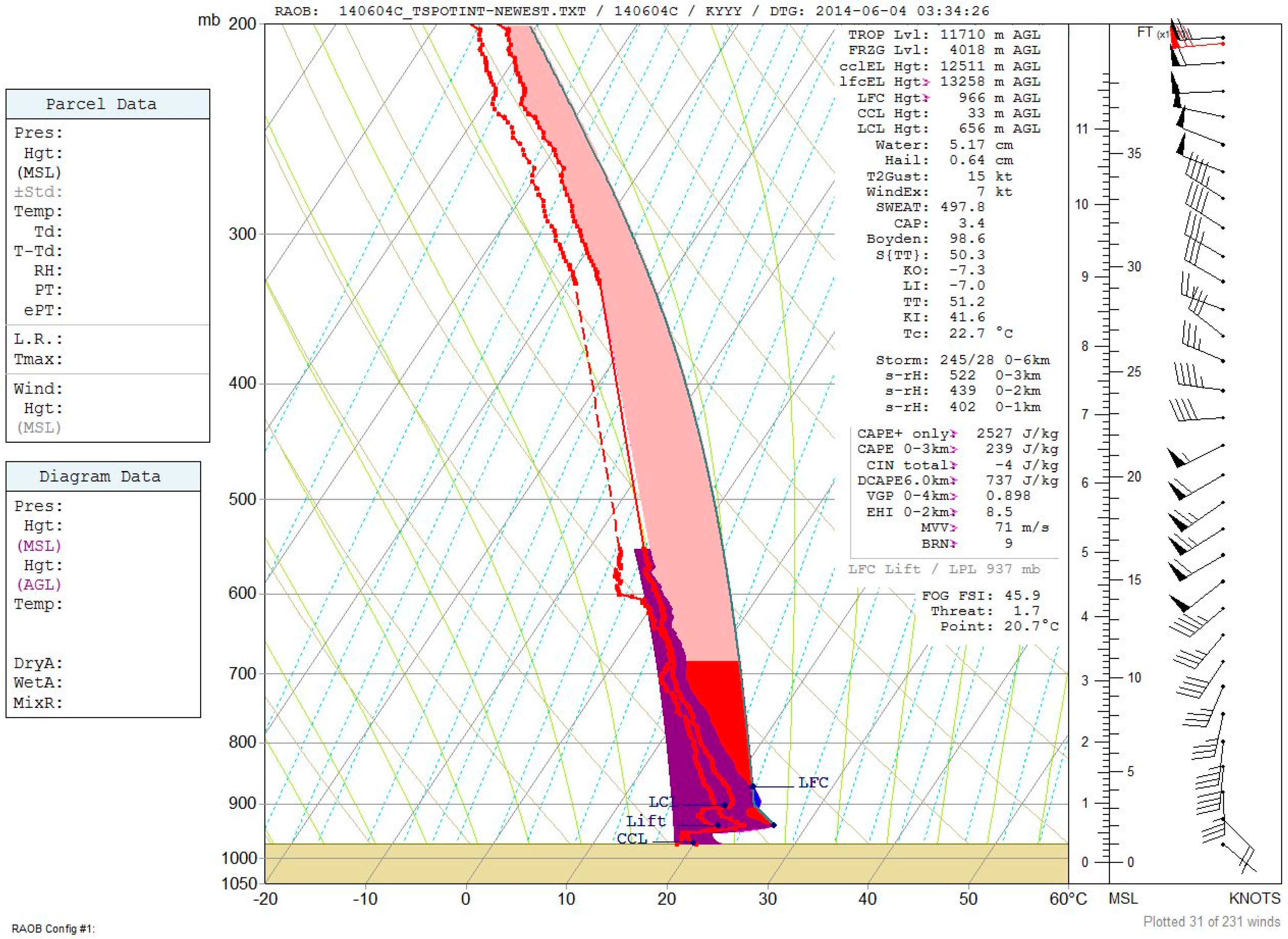
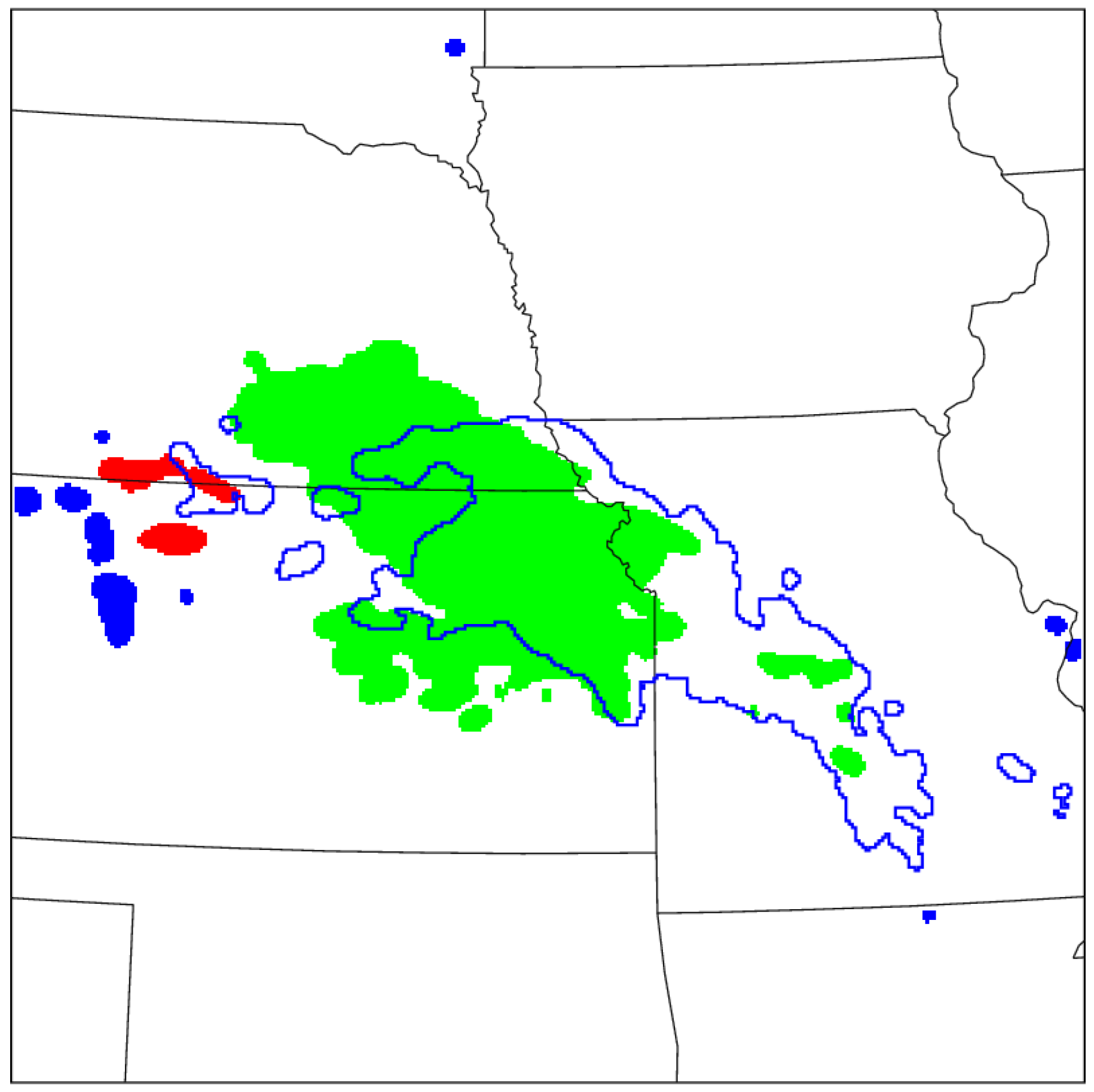
4.2. IOP 2: 3–4 June 2014

A weak leeside low and attendant boundary were present across western Kansas and eastern Colorado. A low-level jet oriented perpendicularly to this boundary fed moisture north of this boundary, and fueled several rounds of elevated convection. This event featured a large elevated MCS that formed over central Nebraska and rode along and north of a warm front that stretched from western Nebraska into Iowa. No DCIN was present in the area during the duration of the event. Cold pools were able to reach the surface, sharpening the thermal gradient and driving the boundary southward, deeper into the warmer air. As we will see, no DCIN values were analyzed during the duration of this event. The sharper gradient led to an enhanced low-level ascent and the redevelopment of convection. This process led to a wide (250-km) swath of heavy precipitation. This event was a classic example of elevated convection north of a surface boundary, in which the boundary was forced southward. This case featured strong, unified cold pools from a large MCS, in contrast to the cellular type convection observed in IOP 1. It was noted that in IOP 1, the cold pools from convection were not able to penetrate to the surface; therefore, the rain that was falling had a minimal and localized cooling effect. This was starkly different in IOP 2, as we see clear evidence of cold pools reaching the surface.
Figure 6 shows the Roebber performance diagram for all 48 models for IOP 2, with elevated convection occurring from southern Iowa and northern Missouri. This figure shows all 48 members provided at least somewhat skillful guidance for this event. Figure 7 shows that nine of the top 10 CSI scores came from model configurations with parameterized convection, while nine of the bottom 10 CSI scores came from models with explicit convection configurations. Additionally, six of the top 10 CSI scores came from models with Mellor–Yamada–Kanishi–Niino (MYNN3) PBL scheme, which uses local vertical mixing.
Parameterized convection model configurations (anything with ‘G’ in the name in Table 2) handled the large MCS better than the explicit convection configurations in regard to CSI scores. However, there was a clear over forecast of QPF from all of the parameterized convection configurations, as indicated by all of the parameterized convection configurations to the left of the 1.0 bias line bisecting Figure 6. Figure 8 depicts the MODE analysis for the 1.0-inch threshold and shows that the overforecast is seen in the best performing model configuration, the TNG (29,257 forecasted grid squares compared to 25,415 observed grid squares). MODE analysis reveals that the TNG had a nearly perfect orientation of the 1.0-inch QPF being only 3° different than the observed QPE. The forecast centroid distance was also excellent; it was only 14.61 grid squares away from the observed QPE centroid. Figure 8 illustrates this forecast showing the observed QPE (red color fill) just inside the TNG QPF contour (blue solid line).
Figure 9A shows the preconvective environment from the TNG model valid at 2100 UTC 3 June 2014. Given the presence of significant insolation north of the warm front, only one boundary was drawn from South Dakota through Illinois. However, it should be noted that there is a thermal gradient across Nebraska and northwest Kansas, and a wind shift across Iowa and Missouri that are not represented with a black line. Figure 9B shows the established boundary displaced southward, with a protrusion in the TNG modeled 2-m temperature fields as a result of the elevated MCS. Figure 9C shows how far southward the boundary has been pushed by 1200 UTC 4 June 2014, all the way from central Nebraska to northern Missouri. The reinforcement of low-level cool air by convective cold pools eventually pushed the boundary, which began as a warm front from central Nebraska into central Kansas and Missouri at 2100 UTC 3 June 2014. Twenty-one hours later, it was analyzed as a cold front across central Missouri, at 1800 UTC 4 June 2014. The TNG model configuration had a fairly good representation of the low-level boundary displacement, as is it correctly handled the orientation of convection and the large unified cold pool that initiated the displacement.
By 0600 UTC 4 June 2014, convection was well-established across southern Nebraska through northwest Missouri. Yet, analyses of DCIN at 0600 UTC and 1200 UTC 4 June 2014 (Figure 10A,B) from the TNG model configuration show a lack of DCIN in the area of convection. This implies that convection downdrafts were able to reach the ground and impact the surface boundary and associated weather. Indeed, there is strong evidence of this as large convective cold pools were able to unify and halt the progress of the analyzed warm front and force it southward as a cold front. Soundings, both simulated and observed, indicated that a shallow inversion was present before, during, and after convection. An example of this environment is seen in Figure 11, which shows an observed sounding near Bethany, Missouri at 0400 UTC 4 June 2014, with a shallow but stout (~8 °C warm nose over 20 mb) inversion. This sounding was flown while convection was being reported near the time of launch, and is located just north of the surface warm front. The inversion observed was between 900–950 mb, which is much lower than what was observed during IOP 1 (~825 mb). The shallow nature of the inversion was unable to develop sufficient DCIN (0 J kg−1 in this sounding) to impede even the modest DCAPE values observed between 400–800 J·kg−1. Thus, downdrafts reached the surface, modified the air mass, and retrograded the front.

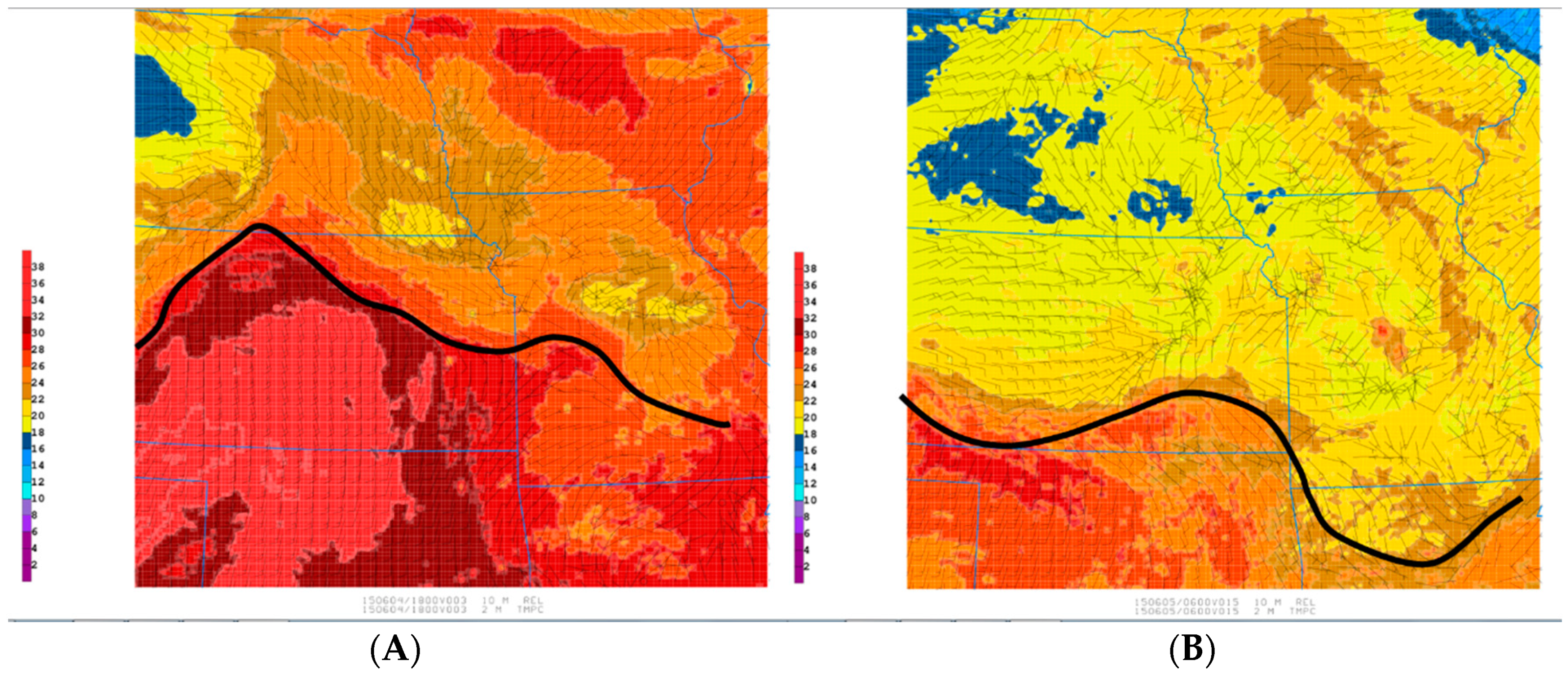
4.3. IOP 5: 4–5 June 2015

This event took place between 4–5 June 2015 across southwest Nebraska into northern Kansas and western Missouri. Elevated convection along and north of the boundary were able to unify and suppress the northeastward advance of the warm front. The meteorological situation is reminiscent of IOP 2, in which a warm front was stalled and forced to retrograde by strong unified elevated convection, which produced cold pools strong that were enough to stall the advancement of the front. As in IOP 2, DCIN was not observed in the area of convection, allowing downdrafts to reach the surface and enhance convection in the interface region of the cold pool—warm front, and drive the front southward.
Figure 12 shows the Roebber performance diagram for the 48 model configurations for IOP 5. The National Centers for Environmental Predication (NCEP) operational guidance (not shown, including the Global Forecast System Model; GFS, North American Mesoscale Model; NAM, and High-Resolution Rapid Refresh Model; HRRR) performed very poorly for this case, spreading far too much QPF into eastern Nebraska and western Iowa. This was similarly observed in most of the WRF-HRHPEFS members and lead to very poor performance among the bulk of the configurations. Most of these poorly performing solutions displaced the bulk of the QPF much too far to the northeast, and continued to have the warm front move slowly northeastward into western Iowa. The notable exception was the strong performing cluster of configurations with WRF microphysics (model configurations 13–18 and 37–48 in Table 2) and parameterized convection. The WSYG, WDYG, WDMG, and WSMG configurations were the only four configurations with CSI scores >0.30, as seen in Figure 12. The WDYG configuration was rated the best, as it had the best bias compared to the others within this cluster. As in IOP 2, the top-performing model configurations for this event included parameterized convection. A cluster of mediocre explicit members showed up around the 0.20 CSI curve, as seen in Figure 12. The very worst-performing members in the lowest left cluster of Figure 12 are made up of configurations with WENO mass and moisture advection schemes and explicit convection.
Figure 13 shows a comparison of the 1.0-inch QPF from the WDYG to the stage IV analysis via MODE. In this figure, all of the shaded areas met or exceeded the 1.0-inch criteria. The different colors are artifacts from the MODE clustering algorithm. The analysis reveals that even the best-performing model configuration had the northern extent of the QPF shield too far to the north, and expanding 1.0 inch of the QPF too far east (as indicated by the centroid distance being off by 47.63 grid squares) into Missouri. That being said, the size (8403 grid squares forecasted versus 8990 grid squares observed) and angle (3.25°) were very well forecasted. The analysis shows the model configuration correctly forecasted the front being forced southeastward, which was something that most of the other model configurations and operational guidance did not indicate.
Convection developed over central Nebraska and paralleled the warm front southeastward. The 2-m temperature field from the top-performing WDYG configuration is shown in Figure 14. It shows a representative atmosphere with two boundaries in the region (a second boundary is located north near the Iowa—Minnesota border). Convection initiated around 2000 UTC 4 June 2015 across south–central Nebraska, and quickly spread southeastward. DCIN values < 0 J kg−1 were not observed, and expectedly, downdrafts were able to reach the surface, bringing cool air to the surface and spreading rapidly south and eastward. Figure 15 shows an observed sounding at 0000 UTC 5 June 2015 that was launched by PRECIP from Nebraska City, Nebraska. Elevated convection was ongoing within 16 km of this sounding at the time of launch, and the location experienced elevated convection within two hours of this launch. This sounding provides an example of an atmosphere that is conducive to elevated convection, yet supportive of enough DCAPE to impact surface weather. In this sounding, we see a prominent warm nose just above 900 mb, increasing 4–5 °C in the span of ~20 mb. Even with this strong inversion present, dominant downdrafts would have been unimpeded, as the DCIN was 0 J kg−1 in this sounding also. By 0600 UTC 5 June 2015, cold pools had expanded southeastward thanks to strong DCAPE, driving the front into southern Kansas. Figure 16A shows the simulated reflectivity and DCIN at 0600 UTC 5 June 2015, which is well into a period of elevated convection occurring across southeast Nebraska, northeast Kansas, and western Missouri. As in IOP 2 discussed previously, DCIN values less than 0 J kg−1 are not observed, indicating that downdrafts should be able to penetrate to the surface. An analysis of DCAPE (Figure 16B) shows much of the region reporting values > 800 J kg−1. Observed soundings from southeast Nebraska and northwest Missouri showed a shallow but pronounced inversion between 925–950 mb. However, strong DCAPE values were able to easily overcome any DCIN present, thus allowing downdrafts to impact surface sensible weather. This is observed as a unified convective cold pool that is easily seen in the 2-m temperature field along the axis of 1+ inch of rainfall. As in IOP 2, the surface boundary was impacted by the convective cold pools, and forced to stall and eventually sag southward. Figure 16B shows that by 1200 UTC 5 June 2015, after hours of heavy rainfall, DCIN was not able to overcome the DCAPE, and downdrafts continued to reach the surface, with the cool air continuing to force the boundary further south. This is seen in Figure 14C, which shows the WDYG 2-m temperature field with the boundary driven southeastward all the way into southern Missouri.

4.4. IOP 8: 8 July 2015

IOP 8 occurred 8 July 2015 over western and central Missouri as a cold front stalled over the Ozark Plateau and began to move northward, while a weak low pressure center moved northeastward from Oklahoma. A large precipitation shield formed in the vicinity of the boundary with the most intense cores forming along and north of the developing warm front as elevated convection.
The best-performing model (with respect to CSI) for IOP 8 at the 1.0-inch threshold was the MNGW configuration, as seen in the Roebber performance diagram (Figure 17). The performance diagram also reveals an interesting pattern in which all of the parameterized convection configurations had bias values near 1.25, and nearly all of the explicit convection configurations had bias values near 1.00. This is likely an artifact of the convective parameterized scheme overproducing convection and trying to create a broader MCS, when in fact the elevated cells were more isolated within a stratiform rain shield. This scenario was similar to that observed in IOP 1, where cells stayed isolated, and the bias was handled better by explicit model configurations in that instance as well. The MODE analysis (Figure 18) confirms the over forecast indicated by the Roebber diagram for the MNGW model configuration.
Figure 19A–C shows the 2-m temperature from the MNGW configuration at 0000 UTC, 0600 UTC, and 1200 UTC on 8 July 2015, respectively. Elevated convection began to intensify over central Missouri by 1200 UTC 8 July 2015. Of note is the lack of a clearly defined cold pool region in the temperature field. This is because DCIN values of less than zero were found, indicating that cold pools would not be able to penetrate to the surface. Figure 20 shows an observed sounding launched by PRECIP from Columbia, Missouri at 1200 UTC 8 July 2015, as elevated convection was occurring. It depicts a deep inversion with a top between 850–875 mb, 90 J kg−1 of DCAPE, and −90 J kg−1 of DCIN.
Figure 21 is an analysis of DCIN, revealing negative values analyzed across northeast Oklahoma and Missouri. At 1200 UTC 8 July 2015, the highest simulated reflectivity values were found in northeast Oklahoma and southwest Missouri along and north of an axis of DCIN values < 50 J kg−1. By 1500 UTC 8 July 2015, the convection had intensified and moved northeast ~160 km, while DCIN values decreased such that much of the convection occurred in an environment with DCIN values < 100 J kg−1. Of note is that convection moved readily to the northeast during this event, and the 2-m temperature field showed no indication of convective cold pools north of the boundary. This was an expected result, as the downdrafts from convection were unable to penetrate significantly to the surface and impact the warm front in the presence of negative DCIN values [10]. This is similar to the pattern that was observed in IOP 1. Indeed, a deep inversion was also observed during this case, with the warm nose maximized near 850 mb.

5. Conclusions

During the PRECIP field campaign, elevated thunderstorms were sampled by radiosondes while events were ongoing. It was observed that some episodes of elevated convection resulted in thunderstorms occurring in an anticipated location, along and north of an advancing warm front. However, several episodes (four of eight total cases intensively studied during PRECIP IOPs) were observed where the boundary was stalled and forced southward as convection north of a boundary laid out large cold pools that dominated surface weather. When this was observed, heavy precipitation was observed where boundaries and cold pools were interacting. Evidence was presented supporting the notion that during some events featuring convection north of a synoptic boundary, significant cold pools were in juxtaposition with warm air to the south of the boundary. This created a scenario in which the cool air north of a surface boundary had convective cold(er) pools embedded within the larger air mass. Enhanced convection and heavy rainfall were observed in these coldest regions that interacted with the warm air along and south of the boundary. Cases in which this was observed occurred in environments that were favorable for elevated MCSs, which is consistent with the results of Moore et al. [2]. Convection was able to sustain itself in this optimal region if cold pools were able to push the boundary south, thus putting the cold air in contact with a fresh, undisturbed warm air environment.
In order to investigate and delineate cases that featured frontal displacement and progression, four of the episodes of elevated convection that were sampled during PRECIP were investigated using a reanalysis ensemble. Two of the episodes were characterized by surface fronts that were stalled and/or forced southward by convective cold pools reaching the ground, while the other two scenarios featured surface boundaries that continued forward progress. A mixed physics approach was used to build the model ensemble (WRF-HRHPEFS) using the Weather Research and Forecasting (WRF) model with the Advanced Research WRF (ARW) core. It contained 48 individual members that varied microphysics, cumulus parameterization, boundary layer physics, and moisture advection schemes. All 48 members of the model were run for the events listed in Table 1. MODE analysis was also performed on these cases, with its analysis providing traditional grid statistics information used to generate Roebber performance diagrams, and comparative information for forecast QPF objects compared to observed stage IV QPE.
An observation emerged from the analyses. In those cases in which DCIN was present (IOP 1 and IOP 8), downdrafts from elevated convection were unable to penetrate to the surface, and the 2-m temperature fields were unaffected. The surface warm front progressed forward with time. Model configurations with explicit convection better simulated these events. For cases that lacked DCIN (IOP 2 and IOP 5), DCAPE was able to overcome the frontal inversion, and convective cold pools were able to merge and impact surface sensible weather. This disruption led to the stalling and/or displacement of the surface boundary. Model configurations with parameterized convection produced better simulations of these episodes. While the number of cases in this study was limited, some evidence is provided for the inclusion of parameterized convection along with explicit convection in a high resolution ensemble, as additional utility could be provided.
The presence of unified surface cold pools north of a boundary clearly has an impact on the movement of the boundary. Boundary displacement seems to be favored when DCAPE values are large enough to overcome the DCIN values found in the inversion layer.
DCIN clearly has potential to be an effective tool in heavy rainfall forecasting, as it can be used to help discern if there is enough DCAPE to generate cold pools that can influence surface weather, including boundary location. This tool also has the potential to be useful for forecasting wind events associated with convection, as suggested by Market et al. [10]. While any thunderstorm has the potential to produce strong, potentially damaging straight-line winds, cases in which |DCIN| > DCAPE are unlikely to allow convective downdrafts to penetrate to the surface, and are therefore unable to produce gusty surface conditions. This is currently under investigation [53]. DCIN should also be investigated in a real-time environment, as it has been shown to have utility in case analysis in this study and the Market et al. [10] study.

Author Contributions

Conceptualization, J.K., P.M. and N.F.; Methodology, J.K. and P.M.; J.K. and P.M.; Software, J.K. and P.M.; Validation, J.K., P.M. and N.F.; Formal Analysis, J.K. and P.M.; Investigation, J.K. and P.M.; Writing-Original Draft Preparation, J.K., P.M.; Writing-Review & Editing, J.K., P.M. and N.F.; Visualization, J.K. and P.M.; Funding Acquisition, P.M. and N.F.

Funding

This research was funded by National Science Foundation (NSF) grant number AGS-1258358.

Acknowledgments

This work is supported in part by the National Science Foundation (NSF), Award No. AGS-1258358. Any opinions, findings, conclusions or recommendations expressed herein are those of the author(s) and do not necessarily reflect the views of NSF. The authors would like to thank all members of the PRECIP who worked as forecasters and field research associates during the project. All observed soundings and raw observed data collected during the project can be found at http://weather.missouri.edu/PRECIP/data.html. The authors would also like to thank the three anonymous reviewers for making suggestions that significantly improved manuscript.

Conflicts of Interest

The authors declare no conflict of interest.

References

  1. Rochette, S.M.; Moore, J.T. Initiation of an Elevated Mesoscale Convective System Associated with Heavy Rainfall. Weather Forecast. 1996, 11, 443–457. [Google Scholar] [CrossRef] [Green Version]
  2. Market, P.S.; Allen, R.S.; Kuligowski, R.; Gruber, A. Precipitation Efficiency of Warm-Season Midwestern Mesoscale Convective Systems. Weather Forecast. 2003, 18, 1273–1285. [Google Scholar] [CrossRef]
  3. Moore, J.T.; Glass, F.H.; Graves, C.E.; Rochette, S.M.; Singer, M.J. The Environment of Warm-Season Elevated Thunderstorms Associated with Heavy Rainfall over the Central United States. Weather Forecast. 2003, 18, 861–878. [Google Scholar] [CrossRef] [Green Version]
  4. McCoy, L.P.; Market, P.S.; Gravelle, C.M.; Graves, C.E.; Fox, N.I.; Rochette, S.M.; Kastman, J.S.; Svoma, B. Composites of Heavy Rain Producing Elevated Thunderstorms in the Central United States. Adv. Meteorol. 2017, 2017, 6932798. [Google Scholar] [CrossRef]
  5. Kastman, J.S.; Market, P.S.; Foscato, A. Rainfall-Lightning Ratio Calculations for Elevated Thunderstorms with Heavy Rainfall. In Proceedings of the Seventh Conference on the Meteorological Applications of Lightning Data, Phoenix, AZ, USA, 4–8 January 2015; American Meteorological Society: Boston, MA, USA, 2015. [Google Scholar]
  6. Kastman, J.S.; Market, P.S.; Fox, N.I.; Foscato, A.L.; Lupo, A.R. Lightning and Rainfall Characteristics in Elevated vs. Surface Based Convection in the Midwest that Produce Heavy Rainfall. Atmosphere 2017, 8, 36. [Google Scholar] [CrossRef]
  7. Kastman, J.S.; McCoy, L.D.; Market, P.S.; Fox, N.I. An example of synergistic coupling of upper-and lower-level jets associated with flash flooding. Meteorol. Appl. 2017, 24, 206–210. [Google Scholar] [CrossRef]
  8. Smull, B.F.; Augustine, J.A. Multiscale Analysis of a Mature Mesoscale Convective Complex. Mon. Weather Rev. 1993, 121, 103–132. [Google Scholar] [CrossRef] [Green Version]
  9. Kastman, J.S.; Market, P.S. The Role of Elevated Thunderstorms in the Poleward Progression of Warm Fronts. In Proceedings of the 27th Conference on Weather Analysis and Forecasting/23rd Conference on Numerical Weather Prediction, Chicago, IL, USA, 28 June–3 July 2015; American Meteorological Society: Boston, MA, USA, 2015. [Google Scholar]
  10. Market, P.S.; Rochette, S.M.; Shewchuk, J.; Difani, R.; Kastman, J.S.; Henson, C.B.; Fox, N.I. Evaluating elevated convection with the downdraft convective inhibition. Atmos. Sci. Lett. 2017, 18, 76–81. [Google Scholar] [CrossRef] [Green Version]
  11. Colman, B.R. Thunderstorms above frontal surfaces in environments without positive CAPE. Part I: A climatology. Mon. Weather Rev. 1990, 118, 1103–1122. [Google Scholar] [CrossRef]
  12. Colman, B.R. Thunderstorms above Frontal Surfaces in Environments without Positive CAPE. Part II: Organization and Instability Mechanisms. Mon. Weather Rev. 1990, 118, 1123–1144. [Google Scholar] [CrossRef] [Green Version]
  13. Grant, B.N. Elevated cold-sector severe thunderstorms: A preliminary study. Natl. Weather Dig. 1995, 19, 25–31. [Google Scholar]
  14. Moore, J.T.; Czarnetzki, A.C.; Market, P.S. Heavy precipitation associated with elevated thunderstorms formed in a convectively unstable layer aloft. Meteorol. Appl. 1998, 5, 373–384. [Google Scholar] [CrossRef]
  15. Corfidi, S.F.; Corfidi, S.J.; Schultz, D.M. Elevated Convection and Castellanus: Ambiguities, Significance, and Questions. Weather Forecast. 2008, 23, 1280–1303. [Google Scholar] [CrossRef] [Green Version]
  16. Corfidi, S.F.; Corfidi, S.J.; Schultz, D.M. Toward a better understanding of elevated convection. In Proceedings of the 23rd Conference on Severe Local Storms, St. Louis, Mo, USA, 5–10 November 2006; American Meteorological Society: Boston, MA, USA, 2016. [Google Scholar]
  17. Nowotarski, C.J.; Markowski, P.M.; Richardson, Y.P. The characteristics of numerically simulated supercell storms situated over statically stable boundary layers. Mon. Weather Rev. 2011, 139, 3139–3162. [Google Scholar] [CrossRef]
  18. Market, P.S. The Program for Research on Elevated Convection with Intense Precipitation (PRECIP): An Overview. In Proceedings of the 28th Conference on Weather Analysis and Forecasting, Seattle, WA, USA, 22–26 January 2017; American Meteorological Society: Boston, MA, USA, 2017; Volume 8B, p. 2. [Google Scholar]
  19. Schumacher, R.S.; Clark, A.J.; Xue, M.; Kong, F. Factors Influencing the Development and Maintenance of Nocturnal Heavy-Rain-Producing Convective Systems in a Storm-Scale Ensemble. Mon. Weather Rev. 2013, 141, 2778–2801. [Google Scholar] [CrossRef] [Green Version]
  20. Corfidi, S.F. Cold Pools and MCS Propagation: Forecasting the Motion of Downwind-Developing MCSs. Weather Forecast. 2003, 18, 997–1017. [Google Scholar] [CrossRef]
  21. Corfidi, S.F.; Meritt, J.H.; Fritsch, J.M. Predicting the Movement of Mesoscale Convective Complexes. Weather Forecast. 1996, 11, 41–46. [Google Scholar] [CrossRef] [Green Version]
  22. Schlemmer, L.; Hohenegger, C. The Formation of Wider and Deeper Clouds as a Result of Cold-Pool Dynamics. J. Atmos. Sci. 2014, 71, 2842–2858. [Google Scholar] [CrossRef] [Green Version]
  23. Droegemeier, K.K.; Wilhelmson, R.B. Numerical Simulation of Thunderstorm Outflow Dynamics. Part I: Outflow Sensitivity Experiments and Turbulence Dynamics. J. Atmos. Sci. 1987, 44, 1180–1210. [Google Scholar] [CrossRef] [Green Version]
  24. Mahoney, W.P., III. Gust front characteristics and the kinematics associated with interacting thunderstorm outflows. Mon. Weather Rev. 1988, 116, 1474–1492. [Google Scholar] [CrossRef]
  25. Jeong, J.-H.; Lee, D.-I.; Wang, C.-C. Impact of Cold Pool on Mesoscale Convective System Produced Extreme Rainfall over southeastern South Korea. Mon. Weather Rev. 2009, 144, 3985–4006. [Google Scholar] [CrossRef]
  26. Billings, J.M.; Parker, M.D. Evolution and maintenance of the 22–23 June 2003 nocturnal convection during BAMEX. Weather Forecast. 2012, 27, 279–300. [Google Scholar] [CrossRef]
  27. Clark, A.J.; Gallus, W.A.; Xue, M.; Kong, F. Convection-Allowing and Convection-Parameterizing Ensemble Forecasts of a Mesoscale Convective Vortex and Associated Severe Weather Environment. Weather Forecast. 2010, 25, 1052–1081. [Google Scholar] [CrossRef] [Green Version]
  28. Done, J.; Davis, C.A.; Weisman, M. The next generation of NWP: Explicit forecasts of convection using the weather research and forecasting (WRF) model. Atmos. Sci. Lett. 2004, 5, 110–117. [Google Scholar] [CrossRef]
  29. Schwartz, C.S.; Kain, J.S.; Weiss, S.J.; Xue, M.; Bright, D.R.; Kong, F.; Thomas, K.W.; Levit, J.J.; Coniglio, M.C.; Wandishin, M.S. Toward Improved Convection-Allowing Ensembles: Model Physics Sensitivities and Optimizing Probabilistic Guidance with Small Ensemble Membership. Weather. Forecast. 2010, 25, 263–280. [Google Scholar] [CrossRef] [Green Version]
  30. Tapiador, F.J.; Tao, W.-K.; Shi, J.J.; Angelis, C.F.; Martinez, M.A.; Marcos, C.; Rodriguez, A.; Hou, A. A Comparison of Perturbed Initial Conditions and Multiphysics Ensembles in a Severe Weather Episode in Spain. J. Appl. Meteorol. Climatol. 2012, 51, 489–504. [Google Scholar] [CrossRef] [Green Version]
  31. Schumacher, R.S. Sensitivity of precipitation accumulation in elevated convective systems to small changes in low-level moisture. J. Atmos. Sci. 2015, 72, 2507–2524. [Google Scholar] [CrossRef]
  32. Schumacher, R.S. Mechanisms for Quasi-Stationary Behavior in Simulated Heavy-Rain-Producing Convective Systems. J. Atmos. Sci. 2009, 66, 1543–1568. [Google Scholar] [CrossRef]
  33. Zhou, X.; Zhu, Y.; Hou, D.; Kleist, D. A Comparison of Perturbations from an Ensemble Transform and an Ensemble Kalman Filter for the NCEP Global Ensemble Forecast System. Weather Forecast. 2016, 31, 2057–2074. [Google Scholar] [CrossRef]
  34. Jirak, I.L.; Weiss, S.J.; Melick, C.J. The SPC storm scale ensemble of opportunity: Overview and results from the 2012 Hazardous Weather Testbed Spring Forecasting Experiment. In Proceedings of the 26th Conference Severe Local Storms, Nashville, TN, USA, 5–8 November 2012; American Meteorological Society: Boston, MA, USA, 2012; Volume P9, p. 137. [Google Scholar]
  35. Schumacher, R.S.; Clark, A.J. Evaluation of Ensemble Configurations for the Analysis and Prediction of Heavy-Rain-Producing Mesoscale Convective Systems. Mon. Weather Rev. 2014, 142, 4108–4138. [Google Scholar] [CrossRef]
  36. Romine, G.S.; Schwartz, C.S.; Berner, J.; Fossell, K.R.; Snyder, C.; Anderson, J.L.; Weisman, M.L. Representing Forecast Error in a Convection-Permitting Ensemble System. Mon. Weather Rev. 2014, 142, 4519–4541. [Google Scholar] [CrossRef]
  37. Skamarock, W.C.; Klemp, J.B.; Dudhia, J.; Gill, D.O.; Barker, D.M.; Duda, M.G.; Huang, X.-Y.; Wang, W.; Powers, J.G. A Description of the Advanced Research WRF Version 3; NCAR Tech. Note NCAR/TN-475+STR; Open Sky Srl: Boulder, CO, USA, 2008; 113p. [Google Scholar] [CrossRef]
  38. Benjamin, S.G.; Weygandt, S.S.; Brown, J.M.; Hu, M.; Alexander, C.R.; Smirnova, T.G.; Olson, J.B.; James, E.P.; Dowell, D.C.; Grell, G.A.; et al. A North American Hourly Assimilation and Model Forecast Cycle: The Rapid Refresh. Mon. Weather Rev. 2016, 144, 1669–1694. [Google Scholar] [CrossRef]
  39. Lin, Y.-L.; Farley, R.D.; Orville, H.D. Bulk Parameterization of the Snow Field in a Cloud Model. J. Clim. Appl. Meteorol. 1983, 22, 1065–1092. [Google Scholar] [CrossRef] [Green Version]
  40. NOAA. National Oceanic and Atmospheric Administration Changes to the NCEP Meso Eta Analysis and Forecast System: Increase in Resolution, New Cloud Microphysics, Modified Precipitation Assimilation, Modified 3DVAR Analysis. 2001. Available online: http://www.emc.ncep.noaa.gov/mmb/mmbpll/eta12tpb/ (accessed on 30 June 2018).
  41. Hong, S.-Y.; Lim, J.-O.J. The WRF single-moment 6-class microphysics scheme (WSM6). J. Korean Meteorol. Soc. 2006, 42, 129–151. [Google Scholar]
  42. Thompson, G.; Field, P.R.; Rasmussen, R.M.; Hall, W.D. Explicit Forecasts of Winter Precipitation Using an Improved Bulk Microphysics Scheme. Part II: Implementation of a New Snow Parameterization. Mon. Weather Rev. 2008, 136, 5095–5115. [Google Scholar] [CrossRef]
  43. Morrison, H.; Thompson, G.; Tatarskii, V. Impact of Cloud Microphysics on the Development of Trailing Stratiform Precipitation in a Simulated Squall Line: Comparison of One- and Two-Moment Schemes. Mon. Weather Rev. 2009, 137, 991–1007. [Google Scholar] [CrossRef]
  44. Lim, K.-S.S.; Hong, S.-Y. Development of an effective double–moment cloud microphysics scheme with prognostic cloud condensation nuclei (CCN) for weather and climate models. Mon. Weather Rev. 2010, 138, 1587–1612. [Google Scholar] [CrossRef]
  45. Grell, G.A.; Freitas, S.R. A scale and aerosol aware stochastic convective parameterization for weather and air quality modeling. Atmos. Chem. Phys. 2014, 14, 5233–5250. [Google Scholar] [CrossRef] [Green Version]
  46. Dudhia, J. 2015: WRF Physics Options. Available online: ftp://ftp.uib.no/pub/gfi/mme085/WRF_LECTURE_SERIES/Dudhia_wrf_physics1.ppt (accessed on 15 July 2018).
  47. Hong, S.-Y.; Noh, Y.; Dudhia, J. A new vertical diffusion package with an explicit treatment of entrainment processes. Mon. Weather Rev. 2006, 134, 2318–2341. [Google Scholar] [CrossRef]
  48. Janjic, Z.I. The Step–Mountain Eta Coordinate Model: Further developments of the convection, viscous sublayer, and turbulence closure schemes. Mon. Weather Rev. 1994, 122, 927–945. [Google Scholar] [CrossRef]
  49. Nakanishi, M.; Niino, H. Development of an improved turbulence closure model for the atmospheric boundary layer. J. Meteorol. Soc. Jpn. 2009, 87, 895–912. [Google Scholar] [CrossRef]
  50. Skamarock, B. 2015: Dynamics Overview and Best Practices. Available online: http://www2.mmm.ucar.edu/wrf/users/workshops/WS2015/ppts/dynamics_skamarock.pdf (accessed on 15 July 2018).
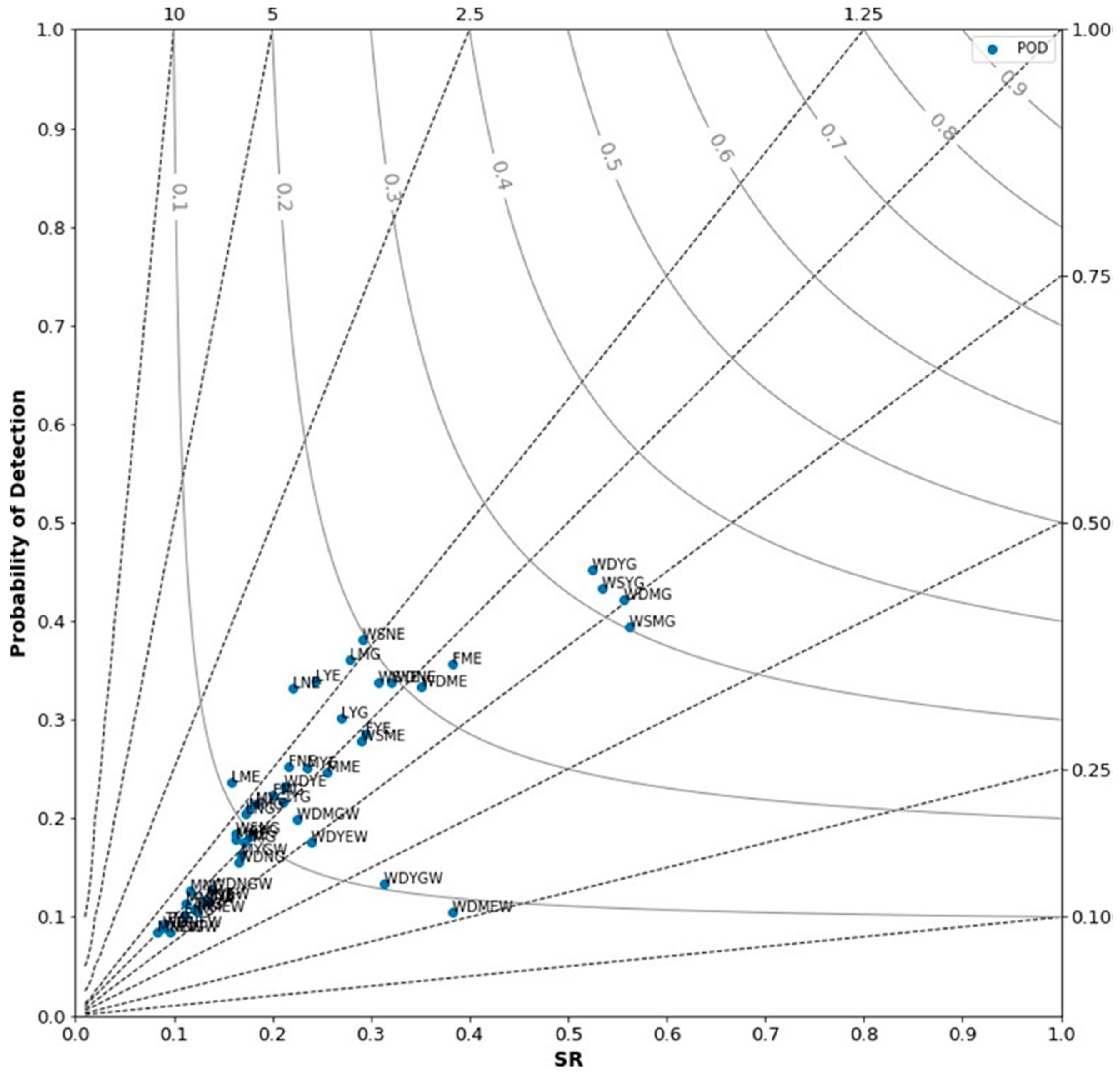
  51. Roebber, P.J. Visualizing multiple measures of forecast quality. Weather Forecast. 2009, 24, 601–608. [Google Scholar] [CrossRef]
  52. Lin, Y.; Mitchell, K.E. The NCEP Stage II/IV hourly precipitation analyses: Development and applications. In Proceedings of the 19th Conference on Hydrology, San Diego, CA, USA, 9–13 January 2005; American Meteorological Society: Boston, MA, USA, 2005; p. 12. [Google Scholar]
  53. Grempler, K.; Market, P.S.; Henson, C.B.; Ritter, S. Using the downdraft convective inhibition (DCIN) to evaluate severe weather threats from elevated convection. In Proceedings of the 29th Conference on Weather Analysis and Forecasting, Denver, CO, USA, 4–8 June 2018; American Meteorological Society: Boston, MA, USA, 2018; Volume 8A, p. 6. [Google Scholar]
Figure 1. An example of downdraft convective available potential energy (DCAPE) and downdraft convective inhibition (DCIN) together in a sounding. The right and left red traces represent the temperature and dew point temperatures, respectively; the purple trace to the right of the temperature trace is the virtual temperature. The convective available potential energy (CAPE) for the most unstable parcel is shaded in red; convective inhibition (CIN), if any, for that same parcel is shaded in light blue; the DCAPE for the coldest wet bulb temperature in the lowest six km is shaded in dark purple; and the DCIN for that same parcel is shaded in a lighter purple. Each of these values is calculated with the virtual temperature correction applied.
Atmosphere 09 00339 g001
Figure 2. Roebber performance diagram showing each member (labeled blue dots) of the WRF-HRHPEFS for IOP 1. The x-axis shows the success ratio (SR), the y-axis shows the probability of detection (POD), the curved lines represent Critical Success Index (CSI) values, and the dashed diagonal lines represent bias. A full description of each member can be found in Table 2.
Atmosphere 09 00339 g002
Figure 3. Method for Object-Based Diagnostic Evaluation (MODE) output showing observed (red color filled area) quantitative precipitation estimate (QPE) and forecast quantitative precipitation forecasts (QPF) (blue outline) from the WDME model configuration for IOP 1.
Atmosphere 09 00339 g003
Figure 4. IOP 1 WDME model configuration forecast of 2-m temperature (color fill, 2 °C interval) and 10-m wind (black solid barbs, valid at (A) 0000 UTC 2 April 2014 and (B) 1800 UTC 2 April 2014. Subjective surface boundary locations indicated by solid black line.
Atmosphere 09 00339 g004
Figure 5. IOP 1 WDME model configuration forecast of DCIN (black solid, 50 J kg−1 interval) and simulated reflectivity over 40 dBZ (grey fill), valid at 1200 UTC 2 April 2014.
Atmosphere 09 00339 g005
Figure 6. As in Figure 2, except of IOP 2.
Atmosphere 09 00339 g006
Figure 7. Sounding from IOP 1 valid 0900 UTC 2 April 2014 for a location near Clinton, Missouri (MO) observed from Program for Research on Elevated Convection with Intense Precipitation (PRECIP) balloon launch. The right and left red traces represent the temperature and dew point temperature, respectively; the purple trace to the right of the temperature trace is the virtual temperature. The convective available potential energy (CAPE) for the most unstable parcel is shaded in red; convective inhibition (CIN), if any, for that same parcel is shaded in light blue; DCAPE for the coldest wet bulb temperature in the lowest 6 km is shaded in dark purple; the DCIN for that same parcel is shaded in a lighter purple. Each of these values is calculated with the virtual temperature correction applied.
Atmosphere 09 00339 g007
Figure 8. As in Figure 3, except for IOP 2.
Atmosphere 09 00339 g008
Figure 9. TNG model configuration forecast of 2-m temperature (color fill, 2 °C interval) and 10-m wind (black solid barbs, valid at (A) 2100 UTC 3 June 2014; (B) 0600 UTC June 2014; and (C) 1200 UTC 4 June 2014. Subjective surface boundary locations indicated by solid black lines.
Atmosphere 09 00339 g009
Figure 10. Contours of DCIN < 0 (black solid, 50 J kg−1 interval) from the TNG model configuration for IOP 2. Valid at (A) 0600 UTC 4 June 2014; and (B) DCIN 1200 UTC 4 June 2014.
Atmosphere 09 00339 g010
Figure 11. 0400 UTC 4 June 2014 sounding launched by PRECIP near Bethany, Missouri. This sounding sampled an environment just north of the surface warm front, and about 25 km south of ongoing convection. The right and left red traces represent the temperature and dew point temperature, respectively; the purple trace to the right of the temperature trace is the virtual temperature. The convective available potential energy (CAPE) for the most unstable parcel is shaded in red; convective inhibition (CIN), if any, for that same parcel is shaded in light blue.
Atmosphere 09 00339 g011
Figure 12. As in Figure 2, except for IOP 5.
Atmosphere 09 00339 g012
Figure 13. MODE output showing observed (red color-filled area) QPE and forecast QPF (blue outline) from the WDYG model configuration for IOP 5. The table at the bottom of the image describes a comparison of the forecasted (blue outline) and observed objects (red, blue, and green color-filled); these values are described in the test.
Atmosphere 09 00339 g013
Figure 14. WDYG model configuration forecast of 2-m temperature (color fill, 2 °C interval) and 10-m wind (black solid barbs), valid at (A) 2100 UTC 4 June 2015; (B) 0600 UTC 5 June 2015; (C) and 1200 UTC 5 June 2015. Subjective surface boundary locations indicated by solid black line symbology.
Atmosphere 09 00339 g014aAtmosphere 09 00339 g014b
Figure 15. Sounding from observed from PRECIP balloon launch during IOP 5 valid 0000 UTC 5 June 2015. Launched near Nebraska City, Nebraska (NE). The right and left red traces represent the temperature and dew point temperature, respectively; the purple trace to the right of the temperature trace is the virtual temperature. The convective available potential energy (CAPE) for the most unstable parcel is shaded in red; convective inhibition (CIN), if any, for that same parcel is shaded in light blue.
Atmosphere 09 00339 g015
Figure 16. WDYG model configuration analyses of simulated reflectivity greater than 35 dBZ (gray shading), valid at 0600 UTC 5 June 2015. Included in (A) is DCAPE (solid black contours, 400 J kg−1 interval), and in (B) is DCIN (solid black contours, 50 J kg−1 intervals).
Atmosphere 09 00339 g016
Figure 17. As in Figure 2, except for IOP 8.
Atmosphere 09 00339 g017
Figure 18. As in Figure 3, except for IOP 8.
Atmosphere 09 00339 g018
Figure 19. IOP 8 MNGW model configuration forecast of 2-m temperature (color fill, 2 °C interval) and 10-m wind (black solid barbs), valid at (A) 2100 UTC 7 July 2015; (B) 0600 UTC 8 July 2015; and (C) 1200 UTC 8 July 2015. Subjective surface boundary locations indicated by solid black lines.
Atmosphere 09 00339 g019aAtmosphere 09 00339 g019b
Figure 20. Observed sounding valid at 1200 UTC 8 June 2015, launched by PRECIP near Columbia, Missouri (MO) during IOP 8. The right and left red traces represent the temperature and dew point temperatures, respectively; the purple trace to the right of the temperature trace is the virtual temperature. The convective available potential energy (CAPE) for the most unstable parcel is shaded in red; convective inhibition (CIN), if any, for that same parcel is shaded in light blue.
Atmosphere 09 00339 g020
Figure 21. IOP 8 WDME model configuration forecasts of DCIN (black solid, 50 J kg−1 interval) and simulated reflectivity over 40 dBZ (grey fill), valid at (A) 1200 UTC 8 July 2015, and (B) 1500 UTC 8 July 2015
Atmosphere 09 00339 g021
Table 1. A listing of the cases discussed throughout this paper. IOP: intense observing period.
DateLocationBrief Synoptic Description
IOP 1: 1–2 April 2014West Central MissouriWarm front lifting northward, front did not stall
IOP 2: 3–4 June 2014Southeast NebraskaWarm front stalled and sank southward
IOP 5: 4–5 June 2015Southeast NebraskaWarm front stalled and sank southward
IOP 8: 7–8 July 2015Central MissouriWarm front lifting northward, front did not stall
Table 2. Weather Research and Forecasting—High Resolution Heavy Precipitation Ensemble Forecasting System (WRF-HRHPEFS) model member configurations name and components of each configuration.
NumberNameICMicrophysicsPBL SchemeCumulus PhysicsAdvection Scheme
1LYERAPLinYUSExplicitPD
2LYGRAPLinYUSGrell 3DPD
3LMERAPLinMYJExplicitPD
4LMGRAPLinMYJGrell 3DPD
5LNERAPLinMYNExplicitPD
6LNGRAPLinMYNGrell 3DPD
7FYERAPFerrierYUSExplicitPD
8FYFRAPFerrierYUSGrell 3DPD
9FMERAPFerrierMYJExplicitPD
10FMGRAPFerrierMYJGrell 3DPD
11FNERAPFerrierMYNExplicitPD
12FNGRAPFerrierMYNGrell 3DPD
13WSYERAPWSM 6YUSExplicitPD
14WSYGRAPWSM 6YUSGrell 3DPD
15WSMERAPWSM 6MYJExplicitPD
16WSMGRAPWSM 6MYJGrell 3DPD
17WSNERAPWSM 6MYNExplicitPD
18WSNGRAPWSM 6MYNGrell 3DPD
19TYERAPThompsonYUSExplicitPD
20TYGRAPThompsonYUSGrell 3DPD
21TMERAPThompsonMYJExplicitPD
22TMGRAPThompsonMYJGrell 3DPD
23TNERAPThompsonMYNExplicitPD
24TNGRAPThompsonMYNGrell 3DPD
25MYERAPMorrisonYUSExplicitPD
26MYGRAPMorrisonYUSGrell 3DPD
27MMERAPMorrisonMYJExplicitPD
28MMGRAPMorrisonMYJGrell 3DPD
29MNERAPMorrisonMYNExplicitPD
30MNGRAPMorrisonMYNGrell 3DPD
31MYEWRAPMorrisonYUSExplicitWENO
32MYGWRAPMorrisonYUSGrell 3DWENO
33MMEWRAPMorrisonMYJExplicitWENO
34MMGWRAPMorrisonMYJGrell 3DWENO
35MNEWRAPMorrisonMYNExplicitWENO
36MNEGRAPMorrisonMYNGrell 3DWENO
37WDYERAPWDM 6YUSExplicitPD
38WDYGRAPWDM 6YUSGrell 3DPD
39WDMERAPWDM 6MYJExplicitPD
40WDMGRAPWDM 6MYJGrell 3DPD
41WDNERAPWDM 6MYNExplicitPD
42WDNGRAPWDM 6MYNGrell 3DPD
43WDYEWRAPWDM 6YUSExplicitWENO
44WDYGWRAPWDM 6YUSGrell 3DWENO
45WDMEWRAPWDM 6MYJExplicitWENO
46WDMGWRAPWDM 6MYJGrell 3DWENO
47WDNEWRAPWDM 6MYNExplicitWENO
48WDMGWRAPWDM 6MYNGrell 3DWENO

